Andreev reflection in the fractional quantum Hall effect

Abstract

We study the reflection of electrons and quasiparticles on point-contact interfaces between fractional quantum Hall (FQH) states and normal metals (leads), as well as interfaces between two FQH states with mismatched filling fractions. We classify the processes taking place at the interface in the strong coupling limit. In this regime a set of quasiparticles can decay into quasiholes on the FQH side and charge excitations on the other side of the junction. This process is analogous to an Andreev reflection in normal-metal/superconductor (N-S) interfaces.

PACS: 73.40.Hm, 71.10.Pm, 73.40.Gk, 73.23.-b

I INTRODUCTION

The first experimental manifestation of the quantized Hall effect came in transport measurements[2]: a precisely defined fractional Hall conductance $\sigma_{xy}=\frac{p}{q}\frac{e^{2}}{h}$ and a vanishing longitudinal conductance $\sigma_{xx}$. These transport properties can be explained by looking at the spectrum of an isolated quantum Hall state. A gauge invariance argument, proposed by Laughlin[3] and elaborated by Halperin[4], relates the existence of a gap for current carrying states to the fractionally quantized Hall conductance $\sigma_{xy}=\frac{p}{q}\frac{e^{2}}{h}$. It is interesting to parallel the case of quantized Hall effects to that of superconductivity, where a transport property, a vanishing resistivity, follows from the existence of an energy gap in the system. In both cases the study of the isolated system, such as the spectrum and quasiparticle excitations, provides the answers for the features observed via transport measurements.

However, as we know for the case of superconductors, there are interesting physical phenomena which arise not from isolated systems, but from the contact of the system with a normal metal. For example, an electron incident from the normal metal side can either be back-reflected at the interface, or be Andreev reflected [5] as a hole and transfer charge $2e$ (a Cooper pair [6]) to the superconductor. It is then very natural to ask whether similar effects can also occur in the case of the FQH effect. More precisely, we should ask what happens in FQH junctions, i.e., when we bring a FQH state in contact with either a normal metal (leads) or another FQH state with different filling fraction.

Some of the properties of these FQH junctions resemble those of normal-metal/superconductor (N-S) junctions, even though the underlying physical reasons are quite different. In the case of Andreev reflection in N-S junctions, an electron incoming from the N side with an energy falling within the superconducting gap cannot go to the S side. It costs a finite energy to create a quasiparticle excitation in the superconductor, but not to create a Cooper pair, so the incoming electron from the N side can be reflected as a hole in the N side, leaving charge $2e$ on the S side of the junction. Here the superconducting gap plays a fundamental role. Now, in the case of FQH junctions, there is a gap for all excitations in the bulk but there are always gapless excitations at the boundary, the edge states. Thus, the mechanism for reflection processes at the boundary does not depend directly on the gap, but instead on the topological properties of FQH states. Consider, for example, a point-contact junction between a $\nu=1/3$ FQH state and either leads or a $\nu=1$ state. Quasiparticles with fractional charge $e^{*}=e/3$ incoming from the $\nu=1/3$ side cannot go to the leads or $\nu=1$ side, for the states on the other side of the junction do not sustain fractionally charged excitations (one may think of this as an infinite gap for charge $e^{*}=e/3$ excitations in a normal metal or a $\nu=1$ state). Thus, upon reaching the junction, a state with two $\nu=1/3$ quasiparticles can (in addition to simply be back-reflected) be reflected as one quasihole with charge $-e/3$ while transmitting charge $e$ to the other side of the junction.

In this paper we will study the different reflection processes taking place at point-contact interfaces between FQH states and normal metals or between two FQH states with different filling fractions. The tools for the study of this problem have been developed in Ref. [7], where the problem of tunneling between two chiral Luttinger liquids with different $g$ parameters was treated by mapping the problem to tunneling between Luttinger liquids with same $g$, and exploring the weak-strong coupling duality symmetry in the latter problem. In that work the problem was studied at the level of the boson fields without considering the underlying Hilbert space for scattering between solitons representing electrons on one side, and fractionally charged quasiparticles on the other.

In what follows we will be able to write the quasiparticle operators before scattering in terms of the chiral boson fields describing the edge excitations. Whereas for weak coupling the quasiparticle operators can still be written in terms of their original chiral boson fields, for strong coupling the boson fields describing both sides of the junction get mixed, and the mixing is determined by the filling fraction mismatch. Using the scattering of quasiparticle operators at the junction we obtain a selection matrix $M$ which relates quantum numbers of incoming and outgoing quasiparticle or soliton states. Such one to one correspondence between in and out quantum numbers exists at both weak and strong coupling limits. We will show that at weak coupling the selection matrix is trivial but at strong coupling it depends on the value of the filling fraction of the FQH system. Although this matrix contains less information than the ${\bf S}$-matrix (which relates amplitudes), it is sufficient to determine transport properties such as the conductance and it allows a classification of the possible processes taking place at the junction. The selection matrix encodes a set of selection rules which we show can be satisfied if the quantum numbers of the scattering states lie on a 2D lattice. At strong coupling the lattice can be described by two basis vectors corresponding to two different reflection processes: normal and Andreev type reflections. The paper is organized as follows: in Sec. II, we describe the model for a FQH-normal metal junction at a point contact. In Sec. III we analyze the model at both fixed points: weak and strong. In Sec. IV we classify the allowed scattering processes at the strong coupling fixed point, in Sec. V we present a conjecture that relates the FQH tunnel junction to the two-channel Kondo problem, and in Sec. VI we review our main results. Details on the proper definition of electron operators and the role of boundary conditions are discussed in the Appendix.

II Formulation of the model

We start with a model Lagrangian for the FQH-normal metal junction at a point-contact which describes the dynamics on the edge of a FQH liquid, the electron gas reservoirs, and the tunneling between them through a single point-contact of the form

$${\cal L}={\cal L}_{edge}+{\cal L}_{res}+{\cal L}_{tun}\,.$$ (1)

The dynamics of the edge of the FQH liquid with a Laughlin filling fraction $\nu=\frac{1}{2k+1}$ is described by a free chiral boson field $\phi_{a}$ with the Lagrangian [8]

$${\cal L}_{edge}=\frac{1}{4\pi}\partial_{x}\phi_{a}(\partial_{t}-\partial_{x})\phi_{a}\,.$$ (2)

The edge electron operator is given by

$$\psi_{edge}\propto\,:e^{-i\frac{1}{\sqrt{\nu}}\phi_{a}(x,t)}:$$ (3)

while the quasiparticle operator is given by

$$\psi_{qp}\propto\,:e^{-i\sqrt{\nu}\phi_{a}(x,t)}:$$ (4)

${\cal L}_{res}$ describes the dynamics of the electron gas reservoir. As shown in Ref. [7], a 2D or 3D electron gas can be mapped to a 1D chiral Fermi liquid (FL) ($\nu=1$) when the tunneling is through a single point-contact. This 1D chiral Fermi liquid is represented by a free chiral boson field $\phi_{b}$. ${\cal L}_{res}$ is given by

$${\cal L}_{res}=\frac{1}{4\pi}\partial_{x}\phi_{b}(\partial_{t}-\partial_{x})\phi_{b}\,.$$ (5)

In this case, the electron operator is given by

$$\psi_{res}\propto:e^{-i\phi_{b}(x,t)}:$$ (6)

In this paper we discuss the problem of tunneling of electrons from the reservoir, or Fermi liquid (FL), to the FQH state and back. Thus, some care has to be taken to keep the correct (anti)commutation relations of the various fields. Naturally the electron operators for the FQH state and the FL must anticommute as they create fermion states. The bosonized formulas for the electron operator for the edge state $\psi_{edge}$ [Eq. (3)] and for the FL [Eq. (6)], as they stand, commute with each other. The conventional way to fix this problem [9] is to multiply each operator by a suitable Klein factor (or cocycle) which ensures the operators have the correct anticommutation properties. The simplest choice is to define two constant boson operators $\eta_{a}$ and $\eta_{b}$ , such that $\eta_{a,b}^{\dagger}\eta_{a,b}=1$; $[\eta_{a},:e^{-i\frac{1}{\sqrt{\nu}}\phi_{a}(x,t)}:]=0$ and $\eta_{a}^{2}=(-1)^{Q_{b}}$, where $Q_{b}$ is the total extra charge at the edge described by $\phi_{b}$ (note that $\eta_{a}$ is defined in terms of $\phi_{b}$, see appendix A). The correct electron operators are then $\psi_{edge}\propto\,\eta_{a}\;:e^{-i\frac{1}{\sqrt{\nu}}\phi_{a}(x,t)}:$ and $\psi_{res}\propto\;\eta_{b}\;:e^{-i\phi_{b}(x,t)}:$ respectively.

The tunneling Lagrangian between the FQH system and the reservoir is

$${\cal L}_{tun}=\Gamma\;\delta(x)\;\eta_{a}^{\dagger}\eta_{b}\;\;:e^{i[\frac{1}{\sqrt{\nu}}\phi_{a}(x,t)-\phi_{b}(x,t)]}:+{\rm h.\ c.\ }\,,$$ (7)

where $\Gamma$ represents the strength of the interaction and the tunneling takes place at $x=0$ in real space. Notice, however, that the product of the Klein factors $\eta_{a}^{\dagger}\eta_{b}$ commutes with all other terms in the Hamiltonian and hence it is a constant of motion and, as such, it can be absorbed in the definition of the tunneling amplitude $\Gamma$. It is also straightforward to show that $\eta_{a}^{\dagger}\eta_{b}$ only changes if the total number of electrons in the combined system, edge plus reservoir, is changed. Thus, from now on, we will drop the Klein factors from the full Hamiltonian.

By folding each chiral boson into a semi-infinite system, one can describe the junction as the coupling between two strings with mismatched Luttinger parameters or compactification radii, as shown in Fig. 1. Such description provides a simple way to obtain the conductance of the junction in terms of the transmission of a pulse due to the mismatched impedances [10] in the case of tied strings ($\Gamma\to\infty$).

FIG. 1.: Two strings with mismatched Luttinger parameters coupled by a tunneling interaction of strength $\Gamma$.

This system has two fixed points: (A) a stable fixed point at $\Gamma=0$ (equivalent to Neumann boundary conditions because there is no current flowing through the junction) and (B) an unstable fixed point at $\Gamma\to\infty$ (a Dirichlet boundary condition because the value of the field at both sides of the junction has to be the same modulo the compactification radii). The first case is trivial, and corresponds to two decoupled systems. The second is solvable via a weak-strong duality symmetry, and we identify in this case the Andreev like processes at the junction.

Since the weak coupling ($\Gamma\to 0$) fixed point is stable, whereas the strong coupling limit ($\Gamma\to\infty$) is unstable, an external voltage or a finite temperature sets a natural energy scale in the problem which then separates the weak and strong coupling regimes. It is thus meaningful to do a perturbative expansion around each fixed point. The small parameters are $\Gamma V^{\frac{1-\nu}{\nu}}$ near $\Gamma=0$ and $\tilde{\Gamma}V^{-\frac{1-\nu}{1+\nu}}$ near $\Gamma\to\infty$, where $\tilde{\Gamma}\propto\Gamma^{-\frac{1+\nu}{2\nu}}$. The crossover at intermediate couplings is non-perturbative but it is accessible through the Bethe Ansatz.

Although this problem can be mapped into a free field plus a single semi-infinite string with a local boundary action (which belongs to a class of integrable models [11, 12]), the complications arise in finding how the original quasiparticles or soliton states transform under the map. In the soliton basis that diagonalizes the semi-infinite string with a local boundary action, the quasiparticles (soliton states) are scattered one by one off the point contact. That is, these quasiparticles diagonalize the interacting Hamiltonian. However they are not the original electrons and Laughlin quasiparticles that are present in the asymptotic scattering states. In fact, these asymptotic scattering states are a complicated combination of the soliton states diagonalizing the interacting Hamiltonian. In this sense, the natural basis for treating the interaction is not the most suitable one to study asymptotic scattering states. In what follows we will focus on the problem of the scattering of asymptotic quasiparticle or soliton states at the junction.

By a suitable rotation, ${\cal L}_{tun}$ can be written as the tunneling Lagrangian between two chiral Luttinger liquids with an effective Luttinger parameter $g^{\prime}$ as follows[7]:

$$\left(\matrix{\varphi_{a}\cr\varphi_{b}}\right)=\left(\matrix{\cos\theta&\sin\theta\cr-\sin\theta&\cos\theta}\right)\left(\matrix{\phi_{a}\cr\phi_{b}}\right)\ ,$$ (8)

with

$$\cos 2\theta=\frac{2\sqrt{\nu}}{1+\nu}\,\;,\;\sin 2\theta=\frac{1-\nu}{1+\nu}$$ (9)

and

$$g^{\prime-1}=\frac{(1+\nu^{-1})}{2}$$ (10)

Because ${\cal L}_{edge}$ and ${\cal L}_{res}$ are invariant under this O(2) rotation, ${\cal L}$ takes the form

$${\cal L} = \frac{1}{4\pi}\partial_{x}\varphi_{a}(\partial_{t}-\partial_{x})\varphi_{a}+\frac{1}{4\pi}\partial_{x}\varphi_{b}(\partial_{t}-\partial_{x})\varphi_{b}$$ (11)

$$\ +\Gamma\,\delta(x)\,e^{i\frac{1}{\sqrt{g^{\prime}}}[\varphi_{a}(x,t)-\varphi_{b}(x,t)]}+h.c.$$ (12)

As Eq. (12) shows, the original problem involving two different fields $\phi_{a}$ and $\phi_{b}$ with compactification radii $R_{a}=\sqrt{\nu}=(2k+1)^{-1/2}$ and $R_{b}=1$ respectively, has been mapped to a problem with two new fields $\varphi_{a}$ and $\varphi_{b}$ with the same compactification radius $R={\sqrt{g^{\prime}}}=(k+1)^{-1/2}$ (see appendix B). This transformation mixes the states of the separate Hilbert spaces of the decoupled systems. Naturally, the rotated states are complicated combinations of products of states in the originally decoupled Hilbert spaces. Furthermore, this operation mixes states with spatial weight even very far away from the tunnel junction.

Notice that the charge being transfered by the tunneling operator in Eq. (12) has still the value of 1 in units of the electron charge $e$. However, the operators $e^{i\varphi_{a,b}/\sqrt{g^{\prime}}}$ have statistics $(k+1)\pi$, and thus have fermionic ($k$ even) or bosonic ($k$ odd) character. Also, notice that the natural eigenstates of the rotated system should be viewed as solitons in terms of the original basis.

Let us remark here that this approach can also be used to describe the more general case of two chiral Luttinger liquids with different filling fractions $\nu_{1}$ and $\nu_{2}$. This case corresponds to the problem of tunneling between the edges of two different FQH systems.

Once this transformation is performed the original interacting Hamiltonian is replaced by two decoupled ones: one of a free field $\varphi_{+}=(\varphi_{a}+\varphi_{b})/\sqrt{2}$ with a conserved current that corresponds to the total charge of the system, and another one $\varphi_{-}=(\varphi_{a}-\varphi_{b})/\sqrt{2}$ with a backscattering interaction. If we use the analogy with strings mentioned above, the field $\varphi_{+}$ describes a string with Neumann boundary conditions at both ends and the field $\varphi_{-}$ describes a string with Neumann boundary conditions at one end and $\Gamma$ boundary conditions at the backscattering point (see Fig. 2). When $\Gamma=0$ this is a Neumann boundary condition and when $\Gamma\rightarrow\infty$ it corresponds to a Dirichlet boundary conditon. Thus, the flow from $\Gamma=0$ to $\Gamma\rightarrow\infty$ can be viewed as the flow from Neumann boundary conditions to Dirichlet boundary conditions. It is on the interacting Hamiltonian for $\varphi_{-}$ where the weak-strong duality transformation [13] is used to study the strong coupling regime.

FIG. 2.: Two strings with different boundary conditions.

III ANALYSIS AT THE FIXED POINTS

A ${\bf\Gamma}=0$ FIXED POINT

Before analyzing the strong coupling regime, we review briefly some well known results from the weak coupling limit $\Gamma=0$. In this regime, the Fermi liquid and the FQH state are decoupled from each other. If an electron (quasiparticle) is sent from the Fermi liquid (FQH) side of the junction it is perfectly reflected at the point contact. Thus there is no net current flowing through the junction in any direction, corresponding to a Neumann boundary condition at the interaction site. In this case the fields used originally to describe electrons and quasiparticle excitations describe both the incoming and the outgoing states and the probability amplitude for any scattering process can be calculated in a straightforward fashion. In a generic scattering process $m$ incoming electrons and $n$ incoming quasiparticles are scattered into $q$ and $p$ electrons and quasiparticles respectively. The probability amplitude for such a process is proportional to:

$$\langle:e^{i\sqrt{\nu}p\phi_{a}^{out}}e^{iq\phi_{b}^{out}}::e^{-i\sqrt{\nu}n\phi_{a}^{in}}e^{-im\phi_{b}^{in}}:\rangle$$ (13)

where $\phi_{a}^{out}=\phi_{a}^{in}$ and $\phi_{b}^{out}=\phi_{b}^{in}$, and the mean value is taken with respect to the quadratic action of the free fields. Because the fields are completely independant in this limit, this probability amplitude can be factorized into two factors:

$$\langle:e^{i\sqrt{\nu}p\phi_{a}^{out}-i\sqrt{\nu}n\phi_{a}^{in}}:\rangle$$ (14)

$$\times\langle:e^{iq\phi_{b}^{out}-im\phi_{b}^{in}}:\rangle$$ (15)

The constraint imposed by charge conservation implies that $p=n$ and $q=m$, so the number of incident electrons (quasiparticles) is the same as the number of outgoing electrons (quasiparticles) and both charges $Q_{a}$ and $Q_{b}$ are conserved independently. This is a perfect reflection process as we already stated. The set of incoming electrons and quasiparticles states can be related to the set of outgoing states, according to charge conservation, by a selection matrix ${\bf M}$:

$$\left(\matrix{q\cr p}\right)={\bf M}\left(\matrix{m\cr n}\right)$$ (16)

The selection matrix ${\bf M}$ transforms the incoming quantum numbers $(m,n)$ into the outgoing ones $(q,p)$. It has the property that ${\bf M}={\bf M}^{-1}$ which is a statement on time reversal symmetry. Since the selection matrix relates only quantum numbers, time reversal in this language does not involve any phase information (which is encoded in the ${\bf S}$-matrix). Notice that in the limit $\Gamma=0$ the selection matrix ${\bf M}$ is the identity matrix ${\bf I}$.

B ${\bf\Gamma}=\infty$ FIXED POINT

In the following we will focus on the strong coupling limit $\Gamma\rightarrow\infty$. The strong coupling limit can be studied using a weak-strong duality transformation [13]. In this limit, the fields $\varphi_{a,b}$ can be written in terms of dual fields ${\tilde{\varphi}}_{a,b}$ defined as

$$\varphi_{a} = \tilde{\varphi}_{a}\Theta(-x)+\tilde{\varphi}_{b}\Theta(x)$$ (17)

$$\varphi_{b} = \tilde{\varphi}_{b}\Theta(-x)+\tilde{\varphi}_{a}\Theta(x)\ .$$ (18)

(here $\Theta(x)$ is the step function).

The Lagrangian describing the dynamics of these fields and their interaction is:

$$\tilde{\cal L} = \frac{1}{4\pi}\partial_{x}\tilde{\varphi}_{a}(\partial_{t}-\partial_{x})\tilde{\varphi}_{a}+\frac{1}{4\pi}\partial_{x}\tilde{\varphi}_{b}(\partial_{t}-\partial_{x})\tilde{\varphi}_{b}$$ (19)

$$+ \tilde{\Gamma}\delta(x)e^{i\sqrt{g^{\prime}}[\tilde{\varphi}_{a}(x,t)-\tilde{\varphi}_{b}(x,t)]}+h.c.$$ (20)

where the usual transformations $g^{\prime}\rightarrow 1/g^{\prime}$ and $\Gamma\rightarrow\tilde{\Gamma}$ have been made. The formulation of the problem in terms of the dual fields ${\tilde{\varphi}}_{a,b}$ has the advantage that, in the strong coupling limit, these are free fields. Thus, the quasiparticles that result as excitations of these fields are non-interacting. However they do not describe the original quasiparticles of the system, given in terms of the fields $\phi_{a}$ (representing FQH excitations) and $\phi_{b}$ (representing Fermi Liquid excitations).

By introducing the fields

$${\tilde{\varphi}}_{\pm}\equiv{\frac{1}{\sqrt{2}}}({\tilde{\varphi}}_{a}\pm{\tilde{\varphi}}_{b})$$ (21)

the Lagrangian describes two decoupled systems

$$\tilde{\cal L} = \tilde{\cal L}_{+}+\tilde{\cal L}_{-}$$ (22)

$$\tilde{\cal L}_{+} = {\frac{1}{4\pi}}\partial_{x}\tilde{\varphi}_{+}(\partial_{t}-\partial_{x})\tilde{\varphi}_{+}$$ (23)

$$\tilde{\cal L}_{-} = \frac{1}{4\pi}\partial_{x}\tilde{\varphi}_{-}(\partial_{t}-\partial_{x})\tilde{\varphi}_{-}$$ (24)

$$+ 2\tilde{\Gamma}\delta(x):\cos(\sqrt{2g^{\prime}}\tilde{\varphi}_{-}(x,t)):$$ (25)

In this representation we see that the FQH tunnel junction is equivalent to the boundary sine-Gordon theory.

It is convenient to invert the rotation described by Eq. (8) so as to define directly free fields $\tilde{\phi}_{a,b}$ dual to the original $\phi_{a,b}$:

$$\phi_{a} = \tilde{\phi}_{a}\Theta(-x)+\big{(}-\sin 2\theta\,\tilde{\phi}_{a}+\cos 2\theta\,\tilde{\phi}_{b}\ )\Theta(x)$$ (26)

$$\phi_{b} = \tilde{\phi}_{b}\Theta(-x)+\big{(}\ \ \ \,\cos 2\theta\,\tilde{\phi}_{a}+\sin 2\theta\,\tilde{\phi}_{b}\ )\Theta(x)$$ (27)

As we stated before, the most general process consists of $m$ incoming electrons, $n$ incoming quasiparticles, scattering into $q$ outgoing electrons and $p$ outgoing quasiparticles ($m,n,p,q$ integers representing the net number of electrons and quasiparticles), as shown in Fig. 3. As in the weak coupling case, the probability amplitude of such a process is proportional to

$$\langle:e^{i\sqrt{\nu}p\phi_{a}^{out}}e^{iq\phi_{b}^{out}}::e^{-i\sqrt{\nu}n\phi_{a}^{in}}e^{-im\phi_{b}^{in}}:\rangle$$ (28)

where the expectation value is taken with respect to a filled Fermi sea of electrons and quasiparticles ($m,n,p,q$ are measured from this level). Using the transformation between the fields and their duals given by Eqs. (26,27), Eq. (28) can be written in terms of the dual fields, which are free fields in the strong coupling limit. Thus Eq. (28) factorizes into a product of two free field expectation values,

$$\langle:e^{i(-\sqrt{\nu}p\sin 2\theta+q\cos 2\theta)\tilde{\phi}_{a}^{out}-i\sqrt{\nu}n\tilde{\phi}_{a}^{in}}:\rangle$$ (29)

$$\times\langle:e^{i(\sqrt{\nu}p\cos 2\theta+q\sin 2\theta)\tilde{\phi}_{b}^{out}-im\tilde{\phi}_{b}^{in}}:\rangle$$ (30)

FIG. 3.: Soliton scattering process from an initial state of $n$ quasiparticles and $m$ electrons to a final state of $p$ quasiparticles and $q$ electrons.

At strong coupling, both charges ${\tilde{Q}}_{a}$ and ${\tilde{Q}}_{b}$, are conserved independently. However, away from strong coupling only the total charge ${\tilde{Q}}_{a}+{\tilde{Q}}_{b}$ is conserved; we will consider this case shortly. For now, we focus on the infinite coupling limit.

As in the weak coupling limit, for a given set $(m,n)$ of electrons and quasiparticles incident on the point-contact, charge conservation imposes a constraint on the allowed quantum numbers $(q,p)$ for the scattered states. This constraint is written in terms of the matrix equation:

$$\left(\matrix{q\cr p}\right)={\bf M}\left(\matrix{m\cr n}\right)\ ,\qquad{\bf M}=\,\left(\matrix{\frac{1-\nu}{1+\nu}&\;\frac{2\nu}{1+\nu}\cr\frac{2}{1+\nu}&\;-\frac{1-\nu}{1+\nu}}\right)\ .$$ (31)

Besides relating incoming and outgoing quantum numbers, the selection matrix ${\bf M}$ also contains information on the non-equilibrium conductance of the point-contact junction. Under the presence of an external voltage a large number $m$ of electrons will be inciding at the junction. The reflection and transmission coefficients for these electrons are respectively:

$$R_{e} =\frac{q}{m}=M_{11}$$ (32)

$$T_{e} =\frac{\nu p}{m}=\nu M_{21}=1-R_{e}\,.$$ (33)

Similarly, (for a reverse applied voltage) the coefficients for $n$ incident quasiparticles at the junction are:

$$R_{qp} =\frac{p}{n}=M_{22}$$ (34)

$$T_{qp} =\frac{\nu^{-1}q}{n}=\nu^{-1}M_{12}=1-R_{qp}\,.$$ (35)

Notice that $T_{qp}>1$ and $R_{qp}<0$. Such enhancement of the transmission, accompanied by a negative reflection coefficient, is also present in N-S junctions because of Andreev reflection. We will make this connection with Andreev scattering more precise once we classify the soliton scattering processes below. Finally, the conductance of the junction is

$$G=\frac{e^{2}}{h}T_{e}=\frac{e^{2}}{h}\nu T_{qp}=\frac{e^{2}}{h}\frac{2\nu}{1+\nu}$$ (36)

in agreement with Refs. [7, 10] (Notice that an external voltage couples to the carriers of the system through their charge. In the case of incident quasiparticles, the charge of the carriers is $\nu$, hence the factor of $\nu$ multiplying $T_{qp}$).

IV CLASSIFICATION OF SCATTERING PROCESSESS AT ${\bf\Gamma}=\infty$ FIXED POINT

The requirement that $m,n,p$, and $q$ be integers constrains $(m,n)$, as well as $(q,p)$, to lie on a lattice (see Fig. 4) that is invariant under the action of the selection matrix ${\bf M}$. Taking $\nu$ to be in the Laughlin’s sequence $\nu=1/(2k+1)$, this lattice can be described using a basis of two vectors

$${\vec{a}}_{1}=(1,1)\,;{\vec{a}}_{2}=(0,k+1)$$ (37)

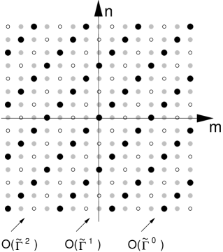
FIG. 4.: Example of the lattice of scattering processes for $\nu=1/7$ ($k=3$) at different orders in $\tilde{\Gamma}$: black circles are zeroth order processes (strong coupling), grey circles are first order and open circles are second order.

Vector ${\vec{a}}_{1}$ represents a process where one incoming electron and one incoming quasiparticle scatter into a final state which is equal to the initial state (see Fig. 5). As a result there is no charge transfer between the QH system and the reservoir through the point contact. This is the process that we will refer to as a normal or perfect reflection.

Vector ${\vec{a}}_{2}$ represents a very different process. In this case $k+1$ incoming quasiparticles are scattered at the point contact into a transmitted electron to the reservoir side and $k$ reflected quasiholes on the QH system side. Although the total charge $Q$ is conserved, there is a net transfer of charge of one electron from the QH system to the reservoir side. It is this process that corresponds to Andreev reflection [5], in analogy with the normal-metal/superconductor (N-S) junction, where an incident electron from the N side with an energy falling within the superconducting gap is back-reflected as a hole while transfering charge $2e$ (a Cooper pair) to the S side. Notice that here the FQH system plays the role of the normal metal (N), whereas the electron gas reservoir (normal metal) plays the role of the superconductor (S). The quasiparticles play the role of the electrons in N and the electrons the role of the Cooper pairs in S. Notice also that the number of quasiparticles and quasiholes involved in the Andreev process for FQH-N junctions depends on the filling fraction (see Fig. 5).

FIG. 5.: Elementary processes at interfaces between a FQH state ($\nu=\frac{1}{2k+1}$) and a normal metal at strong coupling: (a) perfect reflection and (b) Andreev reflection with a net charge transfer.

Our approach to the scattering of incoming and outgoing quasiparticles and electrons at the junction can also be used to address the question of how the properties of the electron gas reservoir are changed due to the strong coupling to the FQH state. For example, a process like $m=q=1,n=p=0$ where one electron is simply reflected by the junction is not allowed in the $\Gamma\to\infty$ limit. However, it is allowed at weak coupling, where any integer pair $(m,n)$ in the plane is accessible. Thus, the strong coupling with a FQH state forbids some of the scattering processes on the Fermi-liquid (FL) side of the junction, making them an inaccessible part of the Hilbert space. Hence, a scattering process of a state with one incoming electron to one outgoing electron on the FL side (without additional excitations on the FQH side) is not allowed and the one-body sector of the ${\bf S}$-matrix vanishes. In other words, the overlap between an incoming state with one electron in the FL and an outgoing state also with one electron in the FL is zero. ${\tilde{\Gamma}}=0$ ($\Gamma\to\infty$) is a non-Fermi liquid fixed point. This behavior is a manifestation of the orthogonality catastrophe in Luttinger liquids.

In what follows, we will show that the crossover between the weak ($\Gamma=0$) and strong (${\tilde{\Gamma}}=0$ or $\Gamma\to\infty$) fixed points can be understood within a simple expansion around ${\tilde{\Gamma}}=0$.

For small $\tilde{\Gamma}$ the dual fields $\tilde{\phi}_{a,b}$ are coupled by the weak perturbation ${\cal L}_{tun}=\tilde{\Gamma}\,\delta(x)\,\cos\left[{ig^{\prime}(\frac{1}{\sqrt{\nu}}\tilde{\phi}_{a}-\tilde{\phi}_{b})}\right]$. The in and out quantum numbers are now related by

$$\left(\matrix{q\cr p}\right)={\bf M}\,\left(\matrix{m\cr n}\right)\ +\ l{\bf t}\ ,\qquad{\bf t}=\left(\matrix{\frac{2\nu}{1+\nu}\cr-\frac{2}{1+\nu}}\right)$$ (38)

and $|l|$ is the order of the expansion ($\tilde{\Gamma}^{|l|}$). Notice that ${\bf Mt}=-{\bf t}$, so that the incoming and outgoing states are related by the same Eq. (38) under time reversal. The allowed values of $(m,n)$ lie on the lattice for $\Gamma\to\infty$ shifted by $\pm|l|$ (Fig. 5). Notice that the tunneling term breaks the independent conservation of the two charges $\tilde{Q}_{a,b}$, conserving only the total charge $\tilde{Q}_{a}+\tilde{Q}_{b}$. Hence, all integer pairs $(m,n)$ in the plane become accessible. From this analysis we see that the strong coupling limit $\Gamma\to\infty$ can be connected to the weak coupling one $\Gamma=0$ continously.

V THE FQH TUNNEL JUNCTION AND QUANTUM IMPURITY PROBLEMS

In this section we will show that it is possible to establish a connection between a Fermi liquid/FQH tunnel junction and a two-channel Kondo problem.

The two-channel Kondo problem is a system in which two species of band fermions (each of them in conventional Fermi liquid states) are coupled, with strength $J$, to a spin-${\frac{1}{2}}$ magnetic impurity localized at the origin. The renormalization group flow of the two-channel Kondo problem has two infrared unstable fixed points, one at $J=0$ and another at $J=\infty$, and a non-trivial infrared stable fixed point at an intermediate value $J_{c}$  [14]. This infrared stable fixed point controls the low energy physics of the two-channel Kondo problem. The physics that emerges from a study of this regime is striking. For instance, it has been shown, first by using Bethe ansatz methods [15, 16] and later on by the more general approach of conformal field theory [17], that the physics at the non-trivial fixed point violates the Fermi liquid hypothesis. Indeed, it was found that the phase controlled by this fixed point is characterized by a finite, non-zero, total entropy at zero temperature, which remains finite in the thermodynamic limit. For the two-channel, spin-${\frac{1}{2}}$ Kondo problem, the entropy is equal to ${\frac{1}{2}}\ln 2$. Moreover, Affleck and Ludwig have also shown that this is a non-Fermi liquid fixed point in the sense that, in this regime, the one-body ${\bf S}$-matrix of the band fermions vanishes at zero frequency. Alternatively stated, the fermion propagator no longer has a pole but a branch cut. It has also been shown that in the two-channel spin-${\frac{1}{2}}$ Kondo problem [18] an anisotropic exchange coupling between the impurity and the conduction electrons is an irrelevant operator, but a perturbation which induces an explicit channel anisotropy and breaks the degeneracy between the two channels, is a relevant operator. The RG flows, due to the presence of the channel symmetry breaking perturbation, drive the system away from the non-trivial zero-temperature fixed point, to a strong coupling (large $J$) and large anisotropy infrared stable fixed point. At this new fixed point the two-channel Kondo system reduces to two decoupled free fermion systems with different boundary conditions: one exhibits the ordinary Kondo effect with complete screening of the impurity and zero ground-state entropy, while the other fermion is completely decoupled from the impurity.

The connection between the FQH junction and the two-channel Kondo problem goes as follows. In Eq. (25) it was shown that the Lagrangian for the FQH tunnel junction is a sum of the Lagrangians of two decoupled systems: a free boson (${\tilde{\varphi}}_{+}$), and a boundary sine-Gordon system (${\tilde{\varphi}}_{-}$) with compactification radius ${\frac{1}{\sqrt{2g^{\prime}}}}={\sqrt{{\frac{k+1}{2}}}}$. From the work of Fendley, Saleur and Warner [19] (FSW), it is known that the boundary sine-Gordon system with this compactification radius has two fixed points: a fixed point at ${\tilde{\Gamma}}=0$ and a fixed point at ${\tilde{\Gamma}}=\infty$. At the ${\tilde{\Gamma}}=0$ fixed point, the boundary operator $:\cos({\sqrt{2g^{\prime}}}{\tilde{\varphi}}_{-}):$ is relevant (with boundary scaling dimension ${\frac{1}{k+1}}$). This operator destabilizes the fixed point and induces an RG flow towards the stable fixed point at ${\tilde{\Gamma}}=\infty$. FSW also found that, at the ${\tilde{\Gamma}}=0$ fixed point, there is a finite ground state entropy equal to $S={\frac{1}{2}}\ln(k+1)$. At the stable fixed point ${\tilde{\Gamma}}=\infty$, the ground state entropy vanishes. Thus we see that, for the special case of $k=1$, we get the same entropy and scaling dimensions as in the two-channel, spin-${\frac{1}{2}}$ Kondo problem. Also, in both problems, FQH/normal metal junctions and two-channel Kondo problem, a given perturbation drives the system from a non-Fermi liquid fixed point to a Fermi liquid fixed point. It is natural then to conjecture that the flow from ${\tilde{\Gamma}}=0$ to ${\tilde{\Gamma}}=\infty$ ( or, equivalently, from $\Gamma=\infty$ to $\Gamma=0$) can be identified with the RG trajectory in the two-channel Kondo problem with channel anisotropy, which flows from the fixed point at $J_{c}$ in the isotropic system to the Kondo fixed point at $J=\infty$ in the extreme anisotropic system.

VI CONCLUSIONS

In this paper we have discussed the physics of tunnel junctions from a Fermi liquid to a single-edge fractional quantum Hall state. The main focus of this work was the problem of scattering of quasiparticles and electrons at the junction. Using the single point contact model of the junction, introduced in Ref. [7], we developed a systematic framework to classify the scattering processes in terms of the incoming and outgoing quantum numbers for the soliton states. We have examined the scattering processes at both the weak and strong tunneling fixed points of the junction.

The physics of the strong coupling fixed point turned out to be quite interesting. We have shown that, at the strong coupling fixed point, there are selection rules that govern the scattering processes. We have described these selection rules in terms of a selection matrix ${\bf M}$ that relates the incoming and outgoing quantum numbers of the excitations. We found that all the scattering processes allowed in the strong coupling limit can be viewed as a combination of two fundamental processes: (a) normal quasiparticle-electron scattering and (b) Andreev processes. In addition to encoding the scattering selection rules, the elements of the matrix ${\bf M}$ give the reflection and transmission coefficients for electrons and quasiparticles at the junction. In particular we have shown that for Andreev processes, which involve several quasiparticles impinging on the junction and resulting on a transmitted electron and a number of reflected quasiholes, there is an enhanced conductance (transmission) and a negative reflection coefficient (on the QH side). This effect is in complete analogy with Andreev reflection in normal-metal/superconductor (N-S) junctions. Notice, however, that the FQH system plays the role of N and the normal metal that of S.

We also find that the constraints imposed by charge conservation at the strong coupling fixed point translate into forbidden processes. For example, the one body ${\bf S}$ matrix for an incoming and outgoing electron in the normal metal side of the junction vanishes at strong coupling. We showed that these processes, however, become accessible as one moves away from infinite coupling. This suggests that the strong coupling fixed point is a non-Fermi liquid fixed point. We then conjecture a possible connection between FQH/normal-metal tunnel junctions and the two-channel spin-$\frac{1}{2}$ Kondo problem. In both problems there is a flow from a non-Fermi liquid fixed point with a finite ground state entropy, to a Fermi liquid fixed point with a vanishing entropy.

We would like to remark here that I. Safi and H. J. Schulz [20] have also discussed an analog of Andreev reflection in tunneling processes into a Luttinger liquid with attractive interactions. (See also the work by Furusaki and Nagaosa [21], who studied tunneling in an inhomogeneous Tomonaga-Luttinger liquid). Although there is a mathematical similarity between the Andreev processes that we discussed in this paper and the processes studied by Safi and Schulz, they are physically quite distinct since, in the context of the QH junctions, Andreev reflection is a consequence of the nature of the QH edge states, which have physically strong repulsive electron-electron interactions. Also, we would like to point out that in the framework that we present, it is possible to classify and describe the quasiparticle (soliton) states which undergo Andreev reflection in addittion to identify the reflection simply by the enhanced conductance.

Note: While this paper was being revised, we became aware of the work by C. Nayak, M. P. A. Fisher, A. W. W. Ludwig and H. H. Lin [22]. In their work, these authors have used the approach described in this paper to describe an enhancement of the tunneling conductance at point contact junctions of multiple Luttinger liquid leads, in terms of Andreev reflection. Also, D. Maslov and P. Goldbart [23] have discussed Andreev processes between two adiabatically connected different non-chiral Luttinger liquids in terms of an enhanced conductance.

VII Acknowledgements

NPS acknowledges D.L.Maslov for helpful discussions and for pointing out the work by Safi and Schulz. This work was supported in part by the NSF through grants NSF DMR94-24511 and NSF DMR-89-20538 at the University of Illinois at Urbana-Champaign (CCC and EF) and by the American Association of University Women (NPS).

A Definition of the electron operator and Klein factors

Here we consider in detail the definition of the electron operator when there is more than one fermionic species present and the introduction of the Klein factors needed in order to satisfy the correct anticonmutation relations between them.

Let us consider a problem with two different types of fermions, ${\it e.g.}$, $\psi_{a}$ and $\psi_{b}$. Because of their fermionic character, they satisfy:

$$\{\psi_{a}(x);\psi_{a}(x^{\prime})\} = 0$$ (A1)

$$\{\psi_{a}(x);\psi_{a}^{\dagger}(x^{\prime})\} = \delta(x-x^{\prime})$$ (A2)

$$\{\psi_{a}(x);\psi_{b}(x^{\prime})\} = 0$$ (A3)

It is clear that the definition $\psi_{a,b}=:e^{-\frac{i}{\sqrt{\nu}}\phi_{a,b}(x)}:$ does not satisfy Eq. (A3) because the boson fields $\phi_{a}$ and $\phi_{b}$ commute. Thus, it is necessary to introduce new fields to obtain the correct commutation relations. We define the electron operator $\psi_{a,b}$ by

$$\psi_{a,b}=\eta_{a,b}{\cal O}_{a,b}$$ (A4)

where the operator ${\cal O}_{i}$ ($i=a,b$) satisfies:

$$\{{\cal O}_{i}(x),{\cal O}_{i}(x^{\prime})\} = 0$$ (A5)

$$\{{\cal O}_{i}(x),{\cal O}_{j}^{\dagger}(x^{\prime})\} = \delta_{ij}\delta(x-x^{\prime})$$ (A6)

$$\bigl{[}\eta_{i},{\cal O}_{j}\bigr{]} = 0$$ (A7)

It can be shown using Eq. (A5, A7), that Eq. (A1) is automatically satisfied for any value of $\eta_{a}$. From Eq. (A2), we see that

$$\{\psi_{a}(x),\psi_{a}^{\dagger}(x^{\prime})\} = \{\eta_{a}{\cal O}_{a}(x),{\cal O}_{a}^{\dagger}(x^{\prime})\eta_{a}^{\dagger}\}$$ (A8)

$$\{\eta_{a}{\cal O}_{a}(x),{\cal O}_{a}^{\dagger}(x^{\prime})\eta_{a}^{\dagger}\} = \eta_{a}\eta_{a}^{\dagger}\delta(x-x^{\prime})$$ (A9)

which is satisfied if $\eta_{a}\eta_{a}^{\dagger}=\eta_{a}^{\dagger}\eta_{a}=1$. By considering that ${\cal O}_{a}(x)=e^{-\frac{i}{\sqrt{\nu}}\phi_{a}(x)}$ we propose that

$$\eta_{a}=e^{i\alpha_{b}p_{\phi_{b}}}$$ (A10)

where $[\phi_{b}(x),p_{\phi_{b}}]=[\phi_{0b},p_{\phi_{b}}]=i$, that is, $p_{\phi_{b}}$ is the zero mode of $\phi_{b}(x)$, and $\alpha_{b}$ is a constant to be determined. Notice that with the normalization chosen, $p_{\phi_{b}}=\sqrt{\nu_{b}}Q_{b}$.

With this definition we can calculate Eq. (A3) as follows:

$$\{\psi_{a}(x),\psi_{b}(x^{\prime})\} = 0$$ (A11)

$$= \{\eta_{a}{\cal O}_{a}(x),\eta_{b}{\cal O}_{b}(x^{\prime})\}$$ (A12)

$$= e^{i\alpha_{b}p_{\phi_{b}}}e^{-\frac{i}{\sqrt{\nu_{a}}}\phi_{a}(x)}e^{i\alpha_{a}p_{\phi_{a}}}e^{-\frac{i}{\sqrt{\nu_{b}}}\phi_{b}(x^{\prime})}+$$ (A14)

$$e^{i\alpha_{a}p_{\phi_{a}}}e^{-\frac{i}{\sqrt{\nu_{b}}}\phi_{b}(x^{\prime})}e^{i\alpha_{b}p_{\phi_{b}}}e^{-\frac{i}{\sqrt{\nu_{a}}}\phi_{a}(x)}$$

Because of the commutation relations between $\phi(x)$ and $p_{\phi}$

$$e^{-\frac{i}{\sqrt{\nu_{j}}}\phi_{j}(x)}e^{i\alpha_{j}p_{\phi_{j}}}=e^{i\frac{\alpha_{j}}{\sqrt{\nu_{j}}}}e^{i\alpha_{j}p_{\phi_{j}}}e^{-\frac{i}{\sqrt{\nu_{j}}}\phi_{j}(x)}$$ (A15)

Using this result in Eq. (A11), the condition:

$$e^{i\frac{\alpha_{a}}{\sqrt{\nu_{a}}}}+e^{i\frac{\alpha_{b}}{\sqrt{\nu_{b}}}}=0$$ (A16)

must be satisfied. It is this condition that determines the values of $\alpha_{a}$ and $\alpha_{b}$:

$$\alpha_{a} = \frac{\pi}{2}\sqrt{\nu_{a}}$$ (A17)

$$\alpha_{b} = -\frac{\pi}{2}\sqrt{\nu_{b}}$$ (A18)

Finally, the $\eta_{a,b}$ operators are defined as:

$$\eta_{a} = e^{i\frac{\pi}{2}Q_{b}}$$ (A19)

$$\eta_{b} = e^{-i\frac{\pi}{2}Q_{a}}$$ (A20)

Notice that the combination entering the tunneling Lagrangian in Eq. (7) is $\eta_{a}^{\dagger}\eta_{b}=e^{-i\frac{\pi}{2}(Q_{a}+Q_{b})}$ and since the total charge $Q_{a}+Q_{b}$ is a constant of motion, it commutes with all the other terms in the Hamiltonian. Also notice that $\eta^{2}=e^{2i\frac{\pi}{2}Q}=(-1)^{Q}$ as expected [24].

B Boundary Conditions and Tunneling

In this appendix we give details on the rotation introduced in Eq. (8), which maps the original fields $\phi_{a}$ and $\phi_{b}$ with different compactification radii to a set of new fields $\varphi_{a}$ and $\varphi_{b}$ with the same compactification radii. We will discuss in some detail the consistency of this rotation with the boundary conditions, imposed by the nature of the FQH state. Here we follow the approach first introduced by X. G. Wen [8] and discussed in considerable detail in the review of ref. [25].

The bosonic fields $\phi_{a,b}$ describe the fluctuations of the edges of a given FQH state. The bulk-edge correspondence [8] implies that, for a Laughlin FQH state with filling fraction $\nu$, the operators $\exp(i(1/\sqrt{\nu})\phi)$ and $\exp(i\sqrt{\nu}\phi)$ (up to Klein factors) are the operators that create electrons (with charge $1$ and Fermi statistics) and QH quasiparticles (of charge $\nu$ and fractional statistics $\pi/\nu$). Hence, the free boson Lagrangian and the electron and quasiparticle operators, are invariant under the translation $\phi\rightarrow\phi+2\pi n{\sqrt{\nu}}$, where $n$ is an integer. The invariance of the states under these translations has to be regarded as a symmetry of the system. Notice that this does not imply that these are the only charged states that can exist at the edge. In fact, since the edge has a gapless spectrum, it is possible to construct local states with any charge. However, these states are not globally defined since only whole electrons can be added or removed from the bulk FQH fluid. Quasiparticles with fractional charge can also be created on the edges but at the expense of creating quasiholes in the bulk in order to maintain charge neutrality; i.e. by insertion of a quantum of flux in the bulk [3]. These facts are reflected in the theory of the edge states through the boundary condition discussed below.

Thus, we will regard states that differ by shifts of $2\pi nR$, with $R={\sqrt{\nu}}$ as being physically identical to each other. In other words, the theory has been “compactified”, giving $\phi$ the character of an angular variable. This property dictates what are the appropriate boundary conditions for the field $\phi$. For an isolated FQH system, which is a droplet of perimeter $L$, the field $\phi$ obeys periodic boundary conditions,

$$\phi(x)=\phi(x+L)$$ (B1)

However, if the amount of charge in the bulk changes, (i. e. by changing the number of electrons or adding a quantum of flux) $\phi$ now satisfies the more general boundary condition

$$\phi(x)=\phi(x+L)+2\pi nR$$ (B2)

We will follow the standard terminology in which $n$ is the winding number of the field configuration and $R$ the compactification radius [26]. Clearly, the boundary condition of Eq. (B2) is consistent with the definition of the electron and quasiparticles operators (vertex operators).

It is worth to remark that the definition of the compactification radius can also be interpreted as the condition for single-valuedness of the electron operator defined on the edges for the closed system. To see this let us consider the change of the electron operator when taken around the droplet of circumference $L$:

$$\psi_{e}(x+L)=e^{i\frac{1}{\sqrt{\nu}}\phi(x+L)}=e^{i\frac{1}{\sqrt{\nu}}\phi(x)}e^{i2\pi n}=\psi_{e}(x)$$ (B3)

However the quasiparticle operator acquires an statistical phase:

$$\psi_{qp}(x+L)=e^{i\sqrt{\nu}\phi(x+L)}=e^{i\sqrt{\nu}\phi(x)}e^{i2\pi n\nu}=e^{i2\pi n\nu}\psi_{qp}(x)$$ (B4)

that is consistent with charge neutrality. As we mentioned above, in order to have a quasiparticle in the edge of the droplet, a quasihole must exist in the bulk. When the quasiparticle is taken around the droplet it picks up an Aharonov-Bhom phase due to the presence of the flux creating the quasihole in the bulk.

The winding number is related to the total charge of the edge as follows. Let $Q$ be the extra charge at the edge due to the excitations, namely

$$Q=\int_{0}^{L}dx\rho(x)=\int_{0}^{L}dx\;{\frac{{\sqrt{\nu}}}{2\pi}}\partial_{x}\phi(x,t)$$ (B5)

Then, consistent with this definition, we get

$$Q=\frac{\sqrt{\nu}}{2\pi}[\phi(x=0,t)-\phi(x=L,t)]=n\nu$$ (B6)

The smallest charge that can be added to the edge is the charge of one quasiparticle (by creating a quasihole in the bulk). In this case $Q=\nu$ and $n$ counts the number of quasiparticles present in the closed system (in this case $n=1$).

In the FQH/normal metal junction we start with two closed systems described by the fields $\phi_{a}$ with winding number $n_{a}$ and compactification radius $R_{a}=\sqrt{\nu}$ and $\phi_{b}$ with winding number $n_{b}$ and compactification radius $R_{b}=1$. The total (extra) charge of the FQH system is $\nu n_{a}$ and the total (extra) charge of the normal metal system is proportional to $n_{b}$. In the presence of tunneling, there is a net charge transfer from one system to the other but the total charge is conserved, therefore we must have the condition

$$\nu n_{a}+n_{b}=0$$ (B7)

Since $n_{b}=1$, because the smallest amount of charge leaving the Fermi liquid side corresponds to one electron, we have $n_{a}=\nu^{-1}=2k+1$.

As we pointed out, the rotation defined in Eq. (8), maps the original fields to the new fields $\varphi_{a}$ with winding number $n^{\prime}_{a}$ and compactification radius $R^{\prime}_{a}$, and $\varphi_{b}$ with winding number $n^{\prime}_{b}$ and compactification radius $R^{\prime}_{b}$. Because these new fields are linear combinations of the original fields, their winding numbers and compactification radii are given by:

$$R^{\prime}_{a}n^{\prime}_{a} = \cos\theta R_{a}n_{a}+\sin\theta R_{b}n_{b}$$ (B8)

$$R^{\prime}_{b}n^{\prime}_{b} = -\sin\theta R_{a}n_{a}+\cos\theta R_{b}n_{b}$$ (B9)

By replacing the expressions for $\cos\theta$, $\sin\theta$, $R_{a}$, $R_{b}$ and the condition $\nu n_{a}+n_{b}=0$, the left hand side of Eq. (B9) is given by:

$$R^{\prime}_{a}n^{\prime}_{a} = \frac{1}{\sqrt{g^{\prime}}}$$ (B10)

$$R^{\prime}_{b}n^{\prime}_{b} = -\frac{1}{\sqrt{g^{\prime}}}$$ (B11)

In the original system we considered the presence of quasiparticles on the edge of the FQH side and tunneling of electrons. In the rotated system we also consider electron tunneling and we allow for the presence of quasiparticles on the edge. By choosing the compactification radius to be: $R^{\prime}_{a,b}=\sqrt{g^{\prime}}$ we get $n^{\prime}=1/g^{\prime}$ that is consistent with the presence of quasiparticles on the edges of the rotated system. Notice that the condition $g^{\prime}(n^{\prime}_{a}+n^{\prime}_{b})=0$ corresponding to the conservation of charge in the rotated system is also automatically satisfied.

REFERENCES

- [1]
- [2] K. von Klitzing, G. Dorda, and M. Pepper, Phys. Rev. Lett. 45, 494 (1980); D. C. Tsui, H. L. Störmer, and A. C. Gossard, Phys. Rev. Lett. 48, 1559 (1982).
- [3] R. B. Laughlin, Phys. Rev. B 23, 5632 (1981).
- [4] B. I. Halperin, Phys. Rev. B 25, 2185 (1982).
- [5] A. F. Andreev, Zh. Eksp. Teor. Fiz. 46, 182 (1964) [Sov. Phys.- JETP 19, 1228 (1964)].
- [6] More precisely, the creation of a Cooper pair is the excitation of a Goldstone mode.
- [7] C. de C. Chamon and E. Fradkin, Phys. Rev. B 56, 2012 (1997).
- [8] X. G. Wen, Phys. Rev. B 41, 12838 (1990).
- [9] M. B. Halpern, Phys. Rev. D 12, 1684 (1975).
- [10] D. B. Chklovskii and B. I. Halperin, cond-mat/9612127.
- [11] S. Ghoshal and A. Zamolodchikov, Int. J. Mod. Phys. A 9, 3841 (1994).
- [12] P. Fendley, A. W. W. Ludwig and H. Saleur, Phys. Rev. B 52, 8934 (1995).
- [13] A. Schmid, Phys. Rev. Lett. 51, 1506 (1983); M. P. A. Fisher and W. Zwerger, Phys. Rev. B 32, 6190 (1985); C. G. Callan and D. E. Freed, Nucl. Phys. B 374, 543 (1992).
- [14] P. Nozieres and A. Blandin, J. Phys. (Paris), 41, 193 (1980).
- [15] N. Andrei and C. Destri, Phys. Rev. Lett. 52, 364 (1984).
- [16] P. B. Wiegmann and A. M. Tsvelik , Z. Phys. 54, 201 (1985).
- [17] I. Affleck and A. W. W. Ludwig, Nucl. Phys. B 352, 849 (1991).
- [18] I. Affleck, A. W. W. Ludwig, H. B. Pang and D. L. Cox, Phys. Rev. B 45, 7918 (1992).
- [19] P. Fendley, H. Saleur and N. Warner, Nucl. Phys. B 430, 577 (1994).
- [20] I. Safi and H. J. Schulz, Phys. Rev. B 52 17040 (1995).
- [21] A. Furusaki and N. Nagaosa, Phys. Rev. B bf 54 R5239 (1996).
- [22] C. Nayak, M. P. A. Fisher, A. W. W. Ludwig and H. H. Lin, cond-mat/9710305.
- [23] D. Maslov and P. Goldbart, cond-mat/9711070.
- [24] F. D. M. Haldane, J. Phys. C 14, 2585 (1981).
- [25] X. G. Wen, Adv. Phys. 44 405 (1995).
- [26] M. Green, J. Schwarz and E. Witten Superstring Theory vol 1, (Cambridge University Press, 1987), p.318-321; P. Di Francesco, P. Mathieu, D. Senechal, Conformal Field Theory (Springer-Verlag New York, 1997), p. 167