Low energy fixed points of the $\sigma$-$\tau$ and the O(3) symmetric Anderson models

Abstract

We study the single channel (compactified) models, the $\sigma$-$\tau$ model and the O(3) symmetric Anderson model, which were introduced by Coleman et al., and Coleman and Schofield, as a simplified way to understand the low energy behaviour of the isotropic and anisotropic two channel Kondo systems. These models display both Fermi liquid and marginal Fermi liquid behaviour and an understanding of the nature of their low energy fixed points may give some general insights into the low energy behaviour of other strongly correlated systems. We calculate the excitation spectrum at the non-Fermi liquid fixed point of the $\sigma$-$\tau$ model using conformal field theory, and show that the results are in agreement with those obtained in recent numerical renormalization group (NRG) calculations. For the O(3) Anderson model we find further logarithmic corrections in the weak coupling perturbation expansion to those obtained in earlier calculations, such that the renormalized interaction term now becomes marginally stable rather than marginally unstable. We derive a Ward identity and a renormalized form of the perturbation theory that encompasses both the weak and strong coupling regimes and show that the $\chi/\gamma$ ratio is 8/3 ($\chi$ is the total susceptibility, spin plus isospin), independent of the interaction $U$ and in agreement with the NRG calculations.

]

I Introduction

In developing a simplified way to understand the low energy behaviour of the isotropic and anisotropic two channel Kondo systems Coleman et al. [1] and Coleman and Schofield [2] introduced two new single channel impurity models. These are the $\sigma$-$\tau$ model and the O(3) symmetric Anderson model. The $\sigma$-$\tau$ model is similar in form to the two channel Kondo model in that a localized spin $s=1/2$ is coupled via an exchange interaction to two conduction electron terms, but only one of these terms is the conduction electron spin $\sigma$, the other term is the conduction electron isospin $\tau$. The Hamiltonian can be expressed in the form,

$$H = [J_{1}\vec{\sigma}(0)+J_{2}\vec{\tau}(0)]\cdot\vec{s}_{d}$$ (2)

$$+\sum_{n=0,\sigma}^{\infty}t_{n}(c^{\dagger}_{{n+1,\sigma}}c_{{n\sigma}}+c^{\dagger}_{{n,\sigma}}c_{{n+1,\sigma}}),$$

where $J_{1}$ and $J_{2}$ are the two exchange couplings, and the conduction electrons are in the form of a tight-binding chain with $c^{\dagger}_{n\sigma}$, $c_{n\sigma}$, the creation and annihilation operators at site $n$, and $t_{n}$ is the nearest neighbour hopping matrix element. The spin operators,

$$\sigma^{+}(n) = c^{\dagger}_{n\uparrow}c_{n\downarrow},\quad\sigma^{-}(n)=c^{\dagger}_{n\downarrow}c_{n\uparrow},\quad$$ (3)

$$\sigma_{\rm z}(n) = {1\over 2}(c^{\dagger}_{n\uparrow}c_{n\uparrow}-c^{\dagger}_{n\downarrow}c_{n\downarrow}),$$ (4)

in the basis spanned by the two singly occupied fermion states, $|0(\uparrow),1(\downarrow)\rangle$ and $|1(\uparrow),0(\downarrow)\rangle$, give a representation for the SU(2) algebra for spin $\sigma={1\over 2}$. The isospin operators,

$$\tau^{+}(n)=(-1)^{n}c^{\dagger}_{n\uparrow}c^{\dagger}_{n\downarrow},\quad\tau^{-}(n)=(-1)^{n}c_{n\downarrow}c_{n\uparrow},$$

$$\tau_{\rm z}(n)={1\over 2}(c^{\dagger}_{n\uparrow}c_{n\uparrow}+c^{\dagger}_{n\downarrow}c_{n\downarrow}-1),$$ (5)

give a representation of the same algebra in the space spanned by the zero and double occupation states, $|0,0\rangle$ and $|1,1\rangle$. The operators for the two conduction electron channels of the two channel Kondo model have been replaced by the operators of a single conduction electron channel, so the term ‘compactified’ has also been used to describe the model. The model as introduced by Coleman et al. was for the isotropic case $J_{1}=J_{2}$.

The O(3) symmetric Anderson model is a modified form of the symmetric Anderson model (SAM). The symmetric Anderson model can be written in the form,

$$H = \sum_{n=0,\sigma}^{\infty}t_{n}(c^{\dagger}_{{n+1,\sigma}}c_{{n\sigma}}+c^{\dagger}_{{n\sigma}}c_{{n+1,\sigma}})$$ (7)

$$+\sum_{\sigma}V(c^{\dagger}_{{0\sigma}}c_{{d\sigma}}+c^{\dagger}_{{d\sigma}}c_{{0\sigma}})+U(n_{d\uparrow}-{1\over 2})(n_{d\downarrow}-{1\over 2}),$$

where $c^{\dagger}_{{d\sigma}}$ and $c_{{d\sigma}}$ are creation and annihilation operators for the localized impurity d state with spin $\sigma$. The electrons in the impurity state interact via a Coulomb matrix element $U$, and $V$ is the hybridization matrix element of the impurity state with a conduction electron chain which is of the same form as that given in (2). This model was modified by Coleman and Schofield [2] by the addition of an anomalous hybridization term,

$$-V_{\rm a}\{c^{\dagger}_{{d\downarrow}}c^{\dagger}_{{0\downarrow}}+c_{{0\downarrow}}c_{{d\downarrow}}+c^{\dagger}_{{d\downarrow}}c_{{0\downarrow}}+c^{\dagger}_{{0\downarrow}}c_{{d\downarrow}}\}.$$ (8)

The motivation for the addition of such a term is that if one applies a Schrieffer-Wolff transformation to the model in the local moment regime (large $U$) then it maps into the $\sigma$-$\tau$ model with $J_{1}$ and $J_{2}$ given by

$$J_{1}={{4V(V-V_{\rm a})}\over{U}},\quad J_{2}={{4VV_{\rm a}}\over{U}}.$$ (9)

The symmetry of the model can be made explicit by the introduction of the Majorana fermion representation. The Majorana fermion operators for the d electrons are defined by

$$d_{1}={1\over{\sqrt{2}}}(c_{d\uparrow}+c^{\dagger}_{d\uparrow}) d_{2}={i\over{\sqrt{2}}}(c_{d\uparrow}-c^{\dagger}_{d\uparrow}),$$ (10)

$$d_{3}={-1\over{\sqrt{2}}}(c_{d\downarrow}+c^{\dagger}_{d\downarrow}) d_{0}={i\over{\sqrt{2}}}(c_{d\downarrow}-c^{\dagger}_{d\downarrow}),$$ (11)

which satisfy the commutation relations,

$$\{d_{\alpha},d_{\beta}\}=\delta_{\alpha,\beta},$$ (12)

where $\{\}$ indicates an anticommutator.

The Majorana operators for the conduction electrons are similarly defined by

$$\psi_{1}(n) = {e^{in\pi/2}\over{\sqrt{2}}}((-1)^{n}c_{n\uparrow}+c^{\dagger}_{n\uparrow}),$$ (13)

$$\psi_{2}(n) = {ie^{in\pi/2}\over{\sqrt{2}}}((-1)^{n}c_{n\uparrow}-c^{\dagger}_{n\uparrow}),$$ (14)

$$\psi_{3}(n) = {-e^{in\pi/2}\over{\sqrt{2}}}((-1)^{n}c_{n\downarrow}+c^{\dagger}_{n\downarrow})$$ (15)

$$\psi_{0}(n) = {ie^{in\pi/2}\over{\sqrt{2}}}((-1)^{n}c_{n\downarrow}-c^{\dagger}_{n\downarrow}),$$ (16)

with commutation relations as in (12). The modified Anderson model in this representation takes the form

$$H = i\sum_{\alpha=1}^{3}V\psi_{\alpha}(0)d_{\alpha}+iV_{0}\psi_{0}(0)d_{0}$$ (17)

$$+ i\sum_{\alpha=0}^{3}\sum_{n=0}^{\infty}t_{n}\psi_{\alpha}(n+1)\psi_{\alpha}(n)+Ud_{1}d_{2}d_{3}d_{0},$$ (18)

where $V_{0}=V-2V_{\rm a}$. The Hamiltonian is invariant under the orthogonal transformation,

$$d_{\alpha}=\sum_{\beta=1}^{3}a_{\alpha,\beta}d_{\beta},\quad\psi_{\alpha}(n)=\sum_{\beta=1}^{3}a_{\alpha,\beta}\psi_{\beta}(n),$$ (19)

where $\sum_{\beta}a_{\alpha,\beta}a_{\alpha^{\prime},\beta}=\delta_{\alpha,\alpha^{\prime}}$ and $\alpha,\alpha^{\prime},\beta=1,2,3$, which corresponds to O(3) symmetry as the 0 Majorana states are not included. For $V_{0}=V$ we recover the standard symmetric Anderson model ($V_{\rm a}=0$) and the model is then symmetric under the corresponding O(4) transformation with the 0 Majorana states included.

These two models do not conserve either the number of particles or the spin. However, there is a combination of spin plus isospin, which we denote by $\vec{j}_{\rm tot}$, which is conserved. For the Anderson model this corresponds to

$$\vec{j}_{\rm tot}=\vec{s}_{d}+\vec{\tau}_{d}+\sum_{n=0}^{\infty}(\vec{\sigma}_{n}+\vec{\tau}_{n}),$$ (20)

where $\vec{\tau}_{d}$ is the isopin operator for the impurity site. As the $\sigma$-$\tau$ model corresponds to the localized limit in which the impurity charge fluctuations are suppressed the $\vec{\tau}_{d}$ is omitted for this model. Clearly this combination satisfies the usual SU(2) angular momentum commutation relations, so the many-body states of these models can be classified by the quantum numbers $j_{\rm tot}$ and $j_{{\rm tot},z}$. The combination of spin and isospin for a particular site $\vec{j}_{n}$ when expressed in terms of the Majorana fermions takes the form,

$$\vec{j}_{n}=\vec{\sigma}_{n}+\vec{\tau}_{n}={{-i}\over{2}}\vec{\psi}(n)\times\vec{\psi}(n),$$ (21)

where $\vec{\psi}(n)=(\psi_{1}(n),\psi_{2}(n),\psi_{3}(n))$. Hence we will refer to the $\alpha=1,2,3$ Majorana components as the components of a vector field, and the $\alpha=0$ as the scalar component.

The $\sigma$-$\tau$ model differs from the two channel Kondo model in that there is no possibility of overscreening the impurity spin. Overscreening occurs in the two channel case in the strong coupling limit $J_{1}\to\infty$, $J_{2}\to\infty$, when a conduction electron in each of the two channels binds to the impurity spin resulting in a localized state at the impurity which again has spin $1/2$. In the $J_{1}\to\infty$, $J_{2}\to\infty$ limit of the $\sigma$-$\tau$ model, however, because the spin and isospin configurations are mutually exclusive states of the same channel the impurity cannot bind to both simultaneously and overcompensation cannot occur.

Coleman et al. established a correspondence between the two models in perturbation theory (after bosonization) and they conjecture that the low energy physics of the two models is essentially the same (see also [3]), with the extra states of the two channel model playing no significant role. For the isotropic case, $J_{1}=J_{2}=J$ they obtained an effective Hamiltonian for the $\sigma$-$\tau$ model by assuming that the low energy fixed point corresponds to $J=\infty$, and then calculating the leading order terms in an expansion in $D/J$ where $D$ is the band width of the conduction electrons. The effective Hamiltonian to leading order in $D/J$ has an interaction term which corresponds to that in the O(3) Anderson model with $U\sim D^{3}/J^{2}$ and $V_{0}=0$, so that corrections to the fixed point correspond to a low order perturbation expansion in powers of $U$ for the O(3) Anderson model. The second order terms generate ${\rm ln}T$ terms in the susceptibility and specific heat, and a Wilson ratio for the logarithmic terms of $8/3$, which is the low energy behaviour of the two channel Kondo model.

There are several reasons why we think these models are worthy of further study. The low order perturbation theory in $U$ (for $V_{0}=0$) gives a self-energy corresponding to the marginal Fermi liquid form whose imaginary part is given by

$${\rm Im}\Sigma^{(2)}(\omega,T)=-{\pi\over 2}\left({U\over{\pi\Delta}}\right)^{2}|\omega|{\rm coth}\left({|\omega|\over{2T}}\right),$$ (22)

and real part,

$${\rm Re}\Sigma^{(2)}(\omega,T)\approx\left({U\over{\pi\Delta}}\right)^{2}\omega{\rm ln}\left({x\over\Delta}\right),$$ (23)

where $x={\rm max}(|\omega|,T)$, $\Delta=\pi V^{2}\rho_{c}(0)$ and $\rho_{c}(0)$ is the density of conduction electron states at the Fermi level [4, 1].

Marginal Fermi liquid theory was put forward in a phenomenological interpretation of the behaviour of the normal state of the high $T_{c}$ superconductors so it is of some interest to understand fully a microscopic model which displays this behaviour [5]. In higher order perturbation theory diagrams were found that give logarithmic contributions to the irreducible four vertex (at zero frequency) with a sign indicating that the weak coupling fixed point [4] might be unstable. It is important to understand the role of these terms in the low energy behaviour of the model, and to determine whether or not the marginal Fermi liquid behaviour corresponds to a stable fixed point. Apart from the non-Fermi liquid behaviour of the isotropic model ($J_{1}=J_{2}$) it has been also conjectured, based on Bethe ansatz calculations, that the behaviour of the anisotropic two channel model also differs from that for a Fermi liquid fixed point [6]. If the $\sigma$-$\tau$ model and the two channel Kondo model have the same low energy fixed point then the anisotropic $\sigma$-$\tau$ should behave in a similar way. These are points that need further clarification.

In the derivation of the low energy behaviour of the $\sigma$-$\tau$ model based on the $1/J$ expansion there are points that are not clear. For the single channel Kondo model it has been shown by Noziéres [7] that, though the low energy fixed point corresponds to $J=\infty$, the low energy physics cannot be calculated from a $1/J$ expansion (which gives a non universal Wilson ratio). We know that for this model there is only one energy scale which is the Kondo temperature $T_{\rm K}$, and so the Wilson ratio ($R$) has a universal value ($R=2$). The effective Hamiltonian that determines the low energy impurity behaviour depends only on $T_{\rm K}$, and asymptotic expansions about the fixed point are in powers of $T/T_{\rm K}$ (or frequency or magnetic field compared to the Kondo temperature). The leading interaction terms in the effective Hamiltonian generated by a $1/J$ expansion do satisfy the Wilson criteria for the leading corrections to the fixed point because (a) they involve operators local to the impurity, and (b) they are consistent with the symmetries of the model. However the combination of these terms generated in this effective Hamiltonian ($D/J\ll 1$), does not correspond to the correct low energy effective Hamiltonian for the Kondo model. The $1/J$ effective Hamiltonian, as to be expected, reproduces the $D/J\ll 1$ physics of the model with a non-universal Wilson ratio dependent upon $D/J$, and so does not give the correct low energy behaviour about the fixed point of the weak coupling model. The applicability of the $1/J$ expansion to derive the excitations about the fixed point of the weak coupling $\sigma$-$\tau$ model needs to be clarified.

In this paper we bring together information on the low energy behaviour of these models, obtained from different many-body techniques, conformal field theory, numerical renormalization group and perturbation theory in order to clarify and resolve some of these outstanding issues. We first of all consider the nature of the excitations in a free single component Majorana chain with various types of boundary conditions, and then calculate possible forms of the many-body excitation spectra when the component systems are put together. We relate these results to those obtained using conformal field theory. The conformal field approach can also be used to calculate the many-body excitations of the isotropic $\sigma$-$\tau$ model for a particular value of the exchange interaction $J=J^{*}$, corresponding to strong coupling. We show that the excitations of the model at this value of $J$ correspond to those found at the fixed point in recent numerical renormalization group calculations [8]. From the conformal field theory we also obtain the form of the operators which give the leading order corrections to this fixed point.

For the O(3) Anderson model we find additional logarithmic terms to those found in earlier work [4], and when these are included the renormalized interaction is marginally irrelevant rather than marginally relevant so the marginal fixed point is stable. We also derive a Ward identity from which we can deduce the Wilson ratio for the total susceptibility (spin plus isospin) of the impurity to the specific heat coefficient. We show that a renormalized perturbation expansion for the Fermi liquid fixed point ($V_{0}\neq 0$) can be generalized for the marginal Fermi liquid fixed point ($V_{0}=0$). The renormalized perturbation theory encompasses both the strong and weak coupling limits. Finally we relate our results to those obtained by other methods, and to the results for the two channel Kondo model.

II Free Majorana Fermion Chain

A Fermi liquid fixed point of an interacting system is characterized by quasiparticle excitations which are in one-to-one correspondence with the single particle excitations of the non-interacting system. In the models we are considering here the single particle excitations of the non-interacting system are independent Majorana fermion excitations. As a preliminary to investigating the fixed point of the interacting systems we look first of all at the possible excitations of a free Majorana chain. We consider just a one component ($\alpha=0$) chain with $N$ sites described by the Hamiltonian,

$$H=it\sum_{n=0}^{N-1}{\psi}_{0}(n){\psi}_{0}(n+1),$$ (24)

where we have taken the hopping matrix-element $t$ (real) to be the same between all neighbouring sites. The number of sites is assumed to be even and we use periodic or antiperiodic boundary conditions ${\psi}_{0}(N)\equiv\pm{\psi}_{0}(0)$.

The Fourier-transformed operators are defined as

$$\bar{\psi}_{0}(k)=\frac{1}{\sqrt{N}}\sum_{n=0}^{N-1}e^{i\frac{2\pi}{N}kn}{\psi}_{0}(n),$$ (25)

We consider first the case of periodic boundary conditions. In this case $k$ takes only the integer values,

$$k=-\frac{N}{2}+1,\ldots,-1,0,1,\ldots,\frac{N}{2}.$$ (26)

The Hamiltonian (24) can be diagonalized by using Eq. (25).

$$H = \sum_{k<0}ite^{i\frac{2\pi}{N}k}\bar{\psi}_{0}(k)\bar{\psi}_{0}(-k)+\sum_{k>0}ite^{i\frac{2\pi}{N}k}\bar{\psi}_{0}(k)\bar{\psi}_{0}(-k)$$ (27)

$$+ it\bar{\psi}_{0}(0)\bar{\psi}_{0}(0)-it\bar{\psi}_{0}(\frac{N}{2})\bar{\psi}_{0}(-\frac{N}{2}).$$ (28)

Due to $\bar{\psi}_{0}(-\frac{N}{2})=\bar{\psi}_{0}(\frac{N}{2})$, the last two terms cancel. There is a Majorana fermion state at the Fermi level but it does not appear explicitly in the Hamiltonian as we take $\mu=0$. For $k>0$ we define the operators

$$\bar{\psi}^{\dagger}_{0}(k)\equiv\bar{\psi}_{0}(-k).$$ (29)

Using Eq. (25) and the commutation relation for the Majorana fermions $\psi_{0}(n)$, one obtains

$$\left\{\bar{\psi}_{0}(k),\bar{\psi}^{\dagger}_{0}(k^{\prime})\right\}_{+}=\delta_{k,k^{\prime}}$$ (30)

which is just the anticommutation relation for ordinary fermion operators. That means that we can treat the operators $\bar{\psi}^{\dagger}_{0}(k)$ and $\bar{\psi}_{0}(k)$ for $k>0$ as fermion operators in the following discussion. The Hamiltonian now takes the simple form

$$H=\sum_{k>0}\epsilon_{k}\bar{\psi}_{0}^{\dagger}(k)\bar{\psi}_{0}(k)+E_{g,{\rm p}},$$ (31)

with the dispersion

$$\epsilon_{k}=2t\sin\frac{2\pi}{N}k$$ (32)

and the ground state energy

$$E_{g,{\rm p}}=it\sum_{k>0}e^{i\frac{2\pi}{N}k}.$$ (33)

In the limit of large $N$, the single particle excitation energies $\epsilon_{k}$ are given by

$$\epsilon_{k}=\frac{4t\pi}{N}k=\frac{\pi v_{\rm F}}{l}k,\ \ k=1,2,3,\ldots.$$ (34)

for small $k/N$. There is a similar linear branch for $k/N\sim{1\over 2}$. The former we will refer to as the left branch and the latter the right branch. Here we have expressed $t$ in terms of the Fermi velocity $v_{\rm F}=2t$ and replaced the number of sites $N$ by the length of the chain $L=N=2l$ (we introduce $l$ to be consistent with the notation used in Sec. III).

The ground state energy is given by

$$E_{g,{\rm p}}=-t\frac{\cos(\frac{\pi}{N})}{\sin(\frac{\pi}{N})}\approx-\frac{v_{\rm F}l}{\pi}\left(1-\frac{1}{12}\frac{\pi^{2}}{l^{2}}\right).$$ (35)

In the case of antiperiodic boundary conditions, $k$ can only take the half-integer values

$$k=-\frac{N}{2}+\frac{1}{2},\ldots,-\frac{1}{2},\frac{1}{2},\ldots,\frac{N}{2}-\frac{1}{2}.$$ (36)

In contrast to Eq. (28) there is no degree of freedom at the Fermi level, so the Hamiltonian reads

$$H=\sum_{k=1/2}^{(N-1)/2}\epsilon_{k}\bar{\psi}_{0}^{\dagger}(k)\bar{\psi}_{0}(k)+E_{g,{\rm a}}$$ (37)

with the dispersion Eq. (32) and the ground state energy

$${E}_{g,a}=it\sum_{k>0}e^{i\frac{2\pi}{N}k}.$$ (38)

In the limit of large $N$, the single particle excitation energies are given by

$$\epsilon_{k}=\frac{\pi v_{\rm F}}{l}k,\ \ k=\frac{1}{2},\frac{3}{2},\frac{5}{2},\ldots.$$ (39)

For the ground state energy we find

$$E_{g,a}=-t\frac{1}{\sin(\frac{\pi}{N})}\approx-\frac{v_{\rm F}l}{\pi}\left(1+\frac{1}{24}\frac{\pi^{2}}{l^{2}}\right).$$ (40)

The difference between the ground state energies for periodic and antiperiodic boundary conditions is

$$E_{g,p}-E_{g,a}=-\frac{v_{\rm F}l}{\pi}\frac{\pi^{2}}{l^{2}}\left(-\frac{1}{12}-\frac{1}{24}\right)=\frac{1}{8}\frac{\pi v_{\rm F}}{l},$$ (41)

where both linearized branches of (37) have been taken into account. With the restriction to only one branch of Majorana fermions, the single particle spectrum is given by Fig. 1(a) and 1(b) for periodic and antiperiodic boundary conditions.

From the single particle spectrum we can also build up the spectrum for the many-body excitations (relative to the ground state) of the scalar Majorana fermion chain, which corresponds to progressively creating ’particles’ in the states with $k\geq 0$. The ground state is a vacuum state with no particles. The ’particles’ which are created are combinations of the usual particle and hole excitations of a free electron system, which are degenerate as a result of the particle-hole symmetry. The resulting many-body energies $E_{\rm ex}$ and their degeneracies $dg$ are given in Tables I and II, where $n_{k}$ denotes the occupation of the single particle state of energy $\epsilon_{k}$.

We can build up the many-body excitations of the vector Majorana fermion chain corresponding to the Hamiltonian,

$$H=it\sum_{n=0}^{N-1}\sum_{\alpha=1}^{3}{\psi}_{\alpha}(n){\psi}_{\alpha}(n+1),$$ (42)

in a similar way. The single particle spectra for this model for periodic and antiperiodic boundary conditions are given in Fig. 2(a) and 2(b), respectively. The number of excited states per energy level is simply multiplied by three as compared to Fig. 1. The resulting many-body states and their degeneracies are given in Table III and IV.

III Conformal Field Theory (CFT)

In this section, we apply a current algebra approach to the channel isotropic $\sigma$-$\tau$ model along the lines developed by Affleck and Ludwig [9] for the two channel Kondo model. In our case, however, a new separation scheme is used in which the conduction electrons, expressed as Majorana fermions, are separated into a density corresponding to total spin (spin plus isospin, the vector channel) and a single (scalar) component Majorana fermion. As in the other examples where this technique is used the model will be solved at a particular finite but large value of the coupling $J^{*}$. At this value of the coupling the impurity spin can be absorbed into the conduction electrons, and the algebra which determines the excitation spectrum is then of the same form as that for the non-interacting system.

The $\sigma$-$\tau$ Hamiltonian can be written as

$$H=it\sum_{n=0}^{\infty}\sum_{\alpha=0}^{3}\psi_{\alpha}(n+1)\psi_{\alpha}(n)+J\vec{j}_{0}\cdot\vec{s}_{d}.$$

where $\vec{j}_{n}$ is the combination of spin and isospin as defined earlier in Eq. (21). In this form the vector and scalar Majorana fermion terms are decoupled so that the model can be divided into two parts (see Fig. 3)

$$H_{\rm sc}=it\sum_{n=0}^{\infty}\psi_{0}(n+1)\psi_{0}(n),$$ (43)

$$H_{\rm vec}=it\sum_{n=0}^{\infty}\sum_{\alpha=1}^{3}\psi_{\alpha}(n+1)\psi_{\alpha}(n)+J\vec{j}_{0}\cdot\vec{s}_{d}.$$ (44)

If the lattice spacing is $a$ we can define a spatial coordinate $x=na$ for each spin and in the limit as $a\to 0$ we use Eqs. (4) and (5) to define both continuum spin and isospin densities with components, $\sigma^{\gamma}(x)$ and $\tau^{\gamma}(x)$, where $\gamma=x,y,z$. These densities satisfy a level $k=1$ $SU(2)$ Kac-Moody algebra:

$$[s^{\alpha}(x),s^{\beta}(x^{\prime})]$$ (45)

$$=i\epsilon^{\alpha\beta\gamma}s^{\gamma}(x)\delta(x-x^{\prime})+\frac{ik}{2\pi}\delta_{\alpha\beta}\delta^{\prime}(x-x^{\prime}).$$ (46)

where $s^{\gamma}(x)=\sigma^{\gamma}(x),\tau^{\gamma}(x)$, and $\delta^{\prime}$ is the derivative of the delta function. If we define similarly a density $\vec{j}(x)$ for the combined spin and isospin then the three components of this density satisfy an $SU(2)$ level $k=2$ Kac-Moody algebra.

In the continuum limit, the linearization of the dispersion relation can be made, and the conduction electrons can be expressed in terms of left- and right-moving Majorana fermions satisfying the conditions $\psi_{\alpha,L}(0)=\psi_{\alpha,R}(0)$ with $\alpha=0,1,2,3$. In fact, one can continue the Majorana fermions to the negative $x$-direction by defining $\psi_{\alpha,L}(x)=\psi_{\alpha,R}(-x)$, so the Hamiltonians can now be written in terms of left-moving fermions only on the full $x$-axis. The Hamiltonian that describes the excitations for the scalar part becomes

$$H_{\rm sc}=\frac{v_{\rm F}}{2\pi}\int_{-\infty}^{\infty}dx:\psi_{0}(x)i\partial_{x}\psi_{0}(x):,$$ (47)

where the subscripts ”L” have been omitted, the Fermi velocity is $v_{\rm F}=2ta$, and $:\hskip 8.5359pt:$ indicates normal ordering. This Hamiltonian has the same form as the one which describes the two dimensional Ising model at the critical point [10].

For the vector part it is possible to apply the standard technique of conformal field theory and write the non-interacting part in the Sugawara form [11], which is quadratic in the densities rather than the fields, so that $H_{\rm vec}$ takes the form,

$$H_{\rm vec}=\frac{v_{\rm F}}{2\pi}\int_{-\infty}^{\infty}dx\left[\frac{1}{4}:\vec{j}(x)\cdot\vec{j}(x):+\frac{2J\pi}{v_{\rm F}}\delta(x)\vec{j}(x)\cdot\vec{s}_{d}\right],$$ (48)

which is normal ordered with respect to the non-interacting system. This Hamiltonian is expressed entirely in terms of the combined spin density $\vec{j}(x)$ and the impurity spin, and is the only part which contains the interaction term.

We choose boundary conditions $\psi_{\alpha}(l)=e^{2i\delta}\psi_{\alpha}(-l)$, on a large circle $-l\leq x\leq l$ for $\alpha=0,1,2,3$. The momenta are then given by $k_{m}=\frac{\pi}{l}\left(m+\frac{\delta}{\pi}\right)$ and the energy levels with respect to the chemical potential are expressed by $E_{m}=v_{\rm F}k_{m}$ with $m=0,\pm 1,\pm 2,\cdot\cdot\cdot$. In the case of particle-hole symmetry, $\delta=0$ corresponds to the case of odd number of sites ($m\in\bf{Z}$, integers) in the lattice version, while $\delta=\pi/2$ to the case of even number sites ($m\in\bf{Z}+\frac{1}{2}$, half-odd integers), these correspond to periodic boundary condition (PBC) and anti-periodic boundary condition (APBC), respectively.

We now look at the $J=0$ case with APBC and PBC. After taking a Fourier transform, the scalar part becomes

$$H_{\rm sc}^{(0)}= \frac{\pi v_{\rm F}}{l}\sum_{m>0}(m+\frac{1}{2})\psi_{0}(-m)\psi_{0}(m)$$ (52)

$$+\left\{\begin{array}[]{ll}-\frac{\pi v_{\rm F}}{l}\frac{c_{\rm sc}}{24},&m\in\bf{Z}+\frac{1}{2}\\ \frac{\pi v_{\rm F}}{l}\frac{c_{\rm sc}}{12},&m\in\bf{Z}\end{array}\right.$$

where $c_{\rm sc}={1\over 2}$ is the central charge of the Virasoro algebra,

$$[L_{n},L_{m}]=(n-m)L_{n+m}+{c\over 12}(n^{3}-n)\delta_{n+m,0},$$ (53)

where $L_{n}$ is the nth component of the mode expansion of the stress-energy tensor, which can be used to generate the excitations of the system (for details see [12]). The eigenvalues of this Hamiltonian can be expressed in the form

$$E_{\rm sc}=\frac{\pi v_{\rm F}}{l}\left[-\frac{1}{48}+\Delta_{\rm Ising}+n_{\rm sc}\right],$$

where $\Delta_{\rm Ising}=0$, $\frac{1}{2}$, $\frac{1}{16}$. This notation is that used in the context of the two dimensional Ising model where the values of $\Delta_{\rm Ising}$ correspond to the scaling dimensions of the primary fields: identity operator $I$, energy density operator $\epsilon$, and Ising order parameter $\sigma$, respectively. For APBC, the first two primary fields appear and each with degeneracy $dg_{\rm sc}=1$. In the PBC case, only $\sigma$ appears with a degeneracy $dg_{\rm sc}=2$. These results agree with those obtained in Tables I and II in the previous section. Those in Table I correspond to $\Delta_{\rm Ising}={1\over 16}$, and in Table II correspond to $\Delta_{\rm Ising}=0,{1\over 2}$.

In terms of the Fourier transform of the spin plus isospin density,

$$\vec{j}(m)=\frac{1}{2\pi}\int_{-l}^{l}dxe^{im\pi x/l}\vec{j}(x),$$

the free vector part may be cast into the form,

$$H_{\rm vec}^{(0)}= \frac{\pi v_{\rm F}}{2l}\sum_{m=1}^{\infty}\vec{j}(-m)\cdot\vec{j}(m)$$ (57)

$$+\frac{\pi v_{\rm F}}{l}\frac{1}{4}\vec{j}(0)\cdot\vec{j}(0)+\left\{\begin{array}[]{ll}-\frac{\pi v_{\rm F}}{l}\frac{c_{\rm vec}}{24},&m\in\bf{Z}+\frac{1}{2}\\ \frac{\pi v_{\rm F}}{l}\frac{c_{\rm vec}}{12},&m\in\bf{Z}\end{array}\right.$$

where $c_{\rm vec}={3\over 2}$ is the central charge for the vector field. The eigenvalues for this part of the Hamiltonian which describes the vector Majorana fermions can be written in the form,

$$E_{\rm vec}=\frac{\pi v_{\rm F}}{l}\left[-\frac{1}{16}+\frac{j(j+1)}{4}+n_{\rm vec}\right],$$

where $j$ is a good quantum number and $n_{\rm vec}$ is a non-negative integer. The primary fields of the conformal field theory corresponding to this model are $j=0$ (singlet), $j=\frac{1}{2}$ (doublet), and $j=1$ (triplet), with scaling dimension $j(j+1)/4$ and degeneracy $dg_{\rm vec}=(2j+1)$. In the PBC case $j=\frac{1}{2}$ and the results correspond to those given in Table III for the excitations relative to the ground state, while for APBC, $j=0,1$ and they correspond to those given in Table IV. The ${\rm O}({1\over l})$ corrections to the ground state energy, which depend on the central charges $c_{\rm sc}$ and $c_{\rm vec}$, are also in agreement with those found in the previous section.

When we put the vector and scalar parts together, the finite-size excitation spectrum of the full model is given by

$$E(j,\Delta_{\rm Ising})=E_{\rm sc}+E_{\rm vec}$$ (58)

$$=\frac{\pi v_{\rm F}}{l}\left[-\frac{1}{12}+\frac{j(j+1)}{4}+\Delta_{\rm Ising}+n_{\rm sc}+n_{\rm vec}\right].$$ (59)

Not all the combinations of the spin and charge degrees of freedom are allowed. Only those combinations representing composite fermions corresponding to the $O(4)$ symmetry of our original free fermion model are allowed. To satisfy this condition the vector part and scalar part should have the same boundary conditions. Therefore, the possible combinations of $(j,\Delta_{\rm Ising})$ are $(0,I)$, $(0,\epsilon)$ or $(1,I)$, and $(1,\epsilon)$ for the APBC ($m\in\bf{Z}+\frac{1}{2}$), while $(\frac{1}{2},\sigma)$ for the PBC ($m\in\bf{Z}$). The finite-size excitation spectra of the non-interacting case for PBC and APBC are shown in Table V and Table VI separately.

We now turn to the case of the interacting model $J\neq 0$. For a particular value of the coupling $J=J^{*}=v_{\rm F}/2$ it is possible to incorporate the impurity spin and define a new spin density $\vec{j^{\prime}}(x)\equiv\vec{j}(x)+2\pi\delta(x)\vec{s}_{d}$ such that the impurity spin operator $\vec{s}_{d}$ disappears explicitly from the Hamiltonian. The vector part of the Hamiltonian is now formally the same as for the non-interacting model,

$$H_{\rm vec}^{*}=\frac{\pi v_{\rm F}}{4l}\sum_{m=-\infty}^{\infty}:\vec{j^{\prime}}(-m)\cdot\vec{j^{\prime}}(m):.$$

The new spin-density operator $\vec{j^{\prime}}(x)$ obeys the same $SU(2)_{2}$ commutation relations as the old one $\vec{j}(x)$ so that at the special point $J=J^{*}$ the same spectrum of excitations are generated for $H_{\rm sc}+H_{\rm vec}^{*}$ in the conformal field algebra as in the non-interacting case. The value of the coupling $J^{*}$ is very large, being of the order of the band width of the conduction electrons, so it corresponds to a strong coupling limit of the original model (see Fig. 4). We are interested in the weak coupling limit of the original model. However, it might describe the fixed point Hamiltonian in a Wilson type of renormalization group calculation (where the energy scale is progressively reduced by eliminating the higher energy states), similar to the case of the s-d (Kondo) model where the fixed point is the strong coupling one. This was conjectured in earlier work [1], and would be consistent with the expectation that the fixed point Hamiltonian should be conformally invariant. In the next section we look at the results of explicit numerical renormalization group calculations that confirm this. Before doing so, however, we will look at physically relevant excitations of the model at $J=J^{*}$. These differ from those already considered for the non-interacting system because, when the impurity spin has been absorbed, the allowed combinations of the vector and scalar excitations are not the same. When we change from $\vec{j}(x)$ to $\vec{j^{\prime}}(x)$, an extra spin ${1\over 2}$ degree of freedom is added to the $SU(2)_{2}$ spin density whereas the quantum numbers of the scalar part are unchanged. The changes in the vector part follow the $SU(2)_{2}$ fusion rule [9]:

$$0\rightarrow\frac{1}{2},\hskip 14.22636pt\frac{1}{2}\rightarrow 0\oplus 1,\hskip 14.22636pt1\rightarrow\frac{1}{2}.$$

As a result, the boundary conditions of the vector part are changed compared to the non-interacting cases: the APBC changes to PBC, while PBC to APBC. Therefore, the boundary conditions of the vector chain and scalar chain are no longer the same. We now have two sets of excitation spectra, which correspond to the combination of the vector part with PBC and scalar part with APBC, or vice versa. These two spectra, which are distinguishable, are displayed in the Table VII and Table VIII, respectively. We will relate these results to those of the numerical renormalization group in the next section.

IV Numerical Renormalization Group (NRG)

The numerical renormalization group method was developed by Wilson for the Kondo problem [13] and later applied to the single impurity Anderson model by Krishnamurthy et al. [14]. It is based on the mapping of the model to a semi-infinite chain with the spin or impurity on one end of the chain coupled to the first conduction electron site via an exchange coupling $J$ or a hybridization $V$. The hopping matrix elements $t_{n}$ between neighbouring sites along the chain approach a constant value for large $n$ as long as the mapping is performed exactly. In the numerical renormalization group, however, certain irrelevant degrees of freedom are neglected which results in an exponential decay $t_{n}\propto\Lambda^{-n/2}$. The origin of the parameter $\Lambda$ is the logarithmic discretization of the continuous conduction band with the energy mesh $\epsilon_{n}=\pm\Lambda^{-n}$, $n=0,1,2,\ldots$. Details of the derivation of the semi-infinite chain form used here can be found in [13] and [14].

Important for the discussion in this paper is the $\Lambda$-dependence of the results due to the logarithmic discretization. As has been shown earlier, the physical properties calculated from the NRG depend only weakly on the discretization parameter $\Lambda$ as long as the number of states taken into account is not too small (usually 500 - 1000). On the other hand, the many-body energy levels at the fixed points are $\Lambda$-dependent. In order to compare the fixed-point spectra with the finite size spectra obtained from the CFT, we have to take the limit $\Lambda\to 1$. This will be discussed in the following subsection.

A The non-Fermi liquid fixed point

We want to concentrate on the fixed point spectra itself, not on the deviations responsible for the $\ln T$-terms in the specific heat and the susceptibility which will be considered in Sec. V. A flow diagram (see also [8]) showing the lowest lying many-body energy levels is presented in Fig. 5 for the isotropic case $V_{\rm a}=V/2$.

The value of the discretization parameter is $\Lambda=2.5$. This diagram shows the crossover from the free-orbital fixed point via the local-moment one to the non-Fermi liquid fixed point. The influence of the local moment fixed point is not great due to the relatively small value of $U$. The excitations of this fixed point are quite different to those found at the Fermi liquid fixed point for $V_{\rm a}\neq V/2$.

In the previous section, the $\sigma$-$\tau$ model was written in terms of Majorana fermions and it was pointed out that in the isotropic case the scalar part of the conduction electron chain is decoupled from the impurity, and that the strong coupling affects only the vector part. As $J\sim V^{2}/U$, this corresponds to the limit $V\to\infty$ of the Anderson model, where V is the hybridization between the vector part of the impurity and the first conduction electron site ($V_{0}=0$). If we start with a total odd number of sites (including the impurity) the effective number of sites remaining is odd in the vector part and even in the scalar part (see also Fig. 4). The effective reduction in the length of the conduction chain at strong coupling changes the excitation spectrum of the vector part in the same way as a change of boundary condition on the free periodic chain. Hence, the combined many-body excitations at this strong coupling point are the same as those calculated via the CFT (see Table VIII).

As the model used in the NRG calculations depends on $\Lambda$ through the hopping matrix element $t_{n}\sim\Lambda^{-n/2}$, the single particle excitations for the free chain for this model depend on $\Lambda$. Our calculations for the free chain in Sec. II and III, however, correspond to $\Lambda=1$. Having identified the low energy fixed point of the $\sigma$-$\tau$ model in terms of the free Majorana chain (with changed boundary conditions), we can use this information to build up the many-body excitations for $\Lambda=2.5$, from the single particle ones ($\Lambda=2.5$) and compare these with those found in the numerical renormalization group calculations ($N\to\infty$). In Fig. 6, the lowest lying many-body energies are calculated from the single particle ones for $\Lambda$ in the range, $1<\Lambda<4$. We can see from this figure that the non-equally spaced excitations go over smoothly to the equally spaced spectrum as $\Lambda\to 1$. The complete agreement of this spectrum (calculated from the single particle spectrum $\Lambda=2.5$) with that calculated from the full NRG calculation confirms the identification of the low energy fixed point of the $\sigma$-$\tau$ model with the strong coupling limit. (However, the NRG gives a ground state degeneracy of four in contrast to the CFT result $dg=2$ (see Table VIII); the origin of this discrepancy is still unclear.)

We want to point out that, in our case, in order to obtain Fig. 6 it was not necessary to run the full NRG-program in the entire $\Lambda$-range. As soon as the relation of single particle and many-body energies has been verified for a certain value of $\Lambda$ the many-body energies can be calculated from the single particle ones for $\Lambda=1$ to compare with the CFT. This is in contrast to the work of Affleck et al. [15] who studied the two channel Kondo model with the NRG. In their case, no relation was made between the fixed point spectrum and the single particle energies of free conduction electron chains so to find the many-body energies to compare with the CFT they had to run the full NRG program for $\Lambda\to 1$. This causes numerical problems as the sequence of iterations does not converge in this limit.

If we start off with a total even number of sites, we get agreement with the CFT results with periodic boundary conditions for the vector part and antiperiodic boundary conditions for the scalar part (see Table VII).

B The Fermi liquid fixed point

For any value of $V_{\rm a}\neq V/2$ the system flows to the Fermi liquid fixed point of the standard single impurity Anderson model defined by $V_{\rm a}=0$ (see the discussion in [8]). Both scalar and vector part of the first conduction electron site are now strongly coupled to the impurity so that the number of effective sites is the same in both the remaining scalar and vector part. The combination of scalar and vector part with the same boundary condition describes the Fermi liquid fixed point, as discussed in the previous section. Again, both the fixed point spectrum and the degeneracies (in the limit $\Lambda\to 1$) are in agreement with the CFT results given in Tables V and VI.

V Leading order corrections to the fixed points

We are primarily interested in the behaviour of the models at the non-Fermi liquid fixed point, which corresponds to $J_{1}=J_{2}$ for the $\sigma$-$\tau$ model and $V_{\rm a}=V/2$ for the O(3) Anderson model. Low order perturbation theory and the numerical renormalization group calculations give a zero point entropy of $\frac{1}{2}\ln 2$, a logarithmic temperature dependence of the specific heat $C(T)\propto T\ln T$ , and a logarithmic temperature dependence of the ‘spin plus isospin’ susceptibility $\chi_{T}(T)\propto\ln T$. In this section we look at arguments that help us to identify the leading irrelevant operators at this fixed point that generate this behaviour.

Because the low energy fixed point of the $\sigma$-$\tau$ model is the strong coupling one, as is the case for the one channel s-d or Kondo model, we can use the analogies between these two to derive an expression for the leading irrelevant operator responsible for the low temperature behaviour. For the ordinary single-channel Kondo model, the leading irrelevant operator is simply ${\vec{J}}^{2}(x=0)$, the squared conserved spin density operator, which is the only $SU(2)$ spin invariant operator with scaling dimension 2. For the present reduced model, we know that the leading irrelevant operator already exists in the non-interacting case where $H_{\rm vec}$, in terms of three-component Majorana fermions with an $SU(2)_{2}$ Kac-Moody algebra, has a supersymmetry associated with the invariance under an exchange of the spin and isospin degrees of freedom, and the corresponding supersymmetric current operator can be defined by $\vec{J}_{s}(x)=i\sqrt{2}\vec{\psi}(x)+\theta\vec{j}(x)$, where $\theta$ is a coordinate which anticommutes with the Majorana operators ($\theta^{2}=1$) [16]. Thus, we have ${\vec{J}_{s}}^{2}(x)\sim\theta\psi_{1}(x)\psi_{2}(x)\psi_{3}(x)$, and from the free field theory we know ${\vec{J}_{s}}^{2}(x)$ is the unique O(3) invariant operator with scaling dimension 3/2. Therefore, we are led to identify the leading irrelevant operator for the reduced single-channel impurity model as ${\vec{J}_{s}}^{2}(x=0)\sim\theta\psi_{1}(0)\psi_{2}(0)\psi_{3}(0)$. As $\theta$ is an anticommuting coordinate one can make a connection with the leading irrelevant operator as calculated by Coleman et al. [1]. In the $1/J$ expansion they find a leading order interaction term of the form $\Phi(0)\psi_{1}(1)\psi_{2}(1)\psi_{3}(1)$ with $\Phi(0)=\psi_{1}(0)\psi_{2}(0)\psi_{3}(0)$. As $\Phi(0)$ is an anticommuting operator it acts in the same way as $\theta$, so one can conclude that they are essentially the same. We discuss this more fully later.

The numerical renormalization group results we have described are for the O(3) Anderson model which, as we discussed in the introduction, is equivalent to the $\sigma$-$\tau$ model in the large $U$ (local moment) regime with $J\sim V^{2}/U$. We have, therefore, interpreted the strong coupling fixed point, in Anderson model terms, as corresponding to the limit $V\to\infty$, which effectively removes the first conduction site from the vector Majorana fermion chain. We end up for both models with the fixed point described by free vector and scalar chains of Majorana fermions with effective lengths which differ by one site. However, the NRG results for the Anderson model for $V_{\rm a}=V/2$ show the same non-Fermi liquid behaviour for all values of $U$. It is possible to give an equivalent interpretation of this fixed point as the $U=0$ limit of the Anderson model. This situation is essentially the same as the $V\to\infty$ one as it corresponds to free vector and scalar Majorana fermion chains whose lengths differ by one site, as only the vector Majorana chain is coupled to the impurity. A similar situation occurs for the standard single channel Anderson model where the fixed point can be interpretated as a Fermi liquid fixed point for all values of $U$. We develop this approach further in Sec. VII.

We now briefly look at the arguments used in the NRG to identify the leading irrelevant operator at the non-Fermi liquid fixed point for the O(3) symmetric Anderson model. We take $H_{N}$ to be the non-interacting model ($U=0)$ with an $N$ site conduction chain, and consider a perturbation of the form,

$$\delta H_{1}=-\tilde{U}\psi_{0}(-1)\psi_{1}(-1)\psi_{2}(-1)\psi_{3}(-1)$$ (60)

where $\psi_{0}(-1)$ is an additional Majorana-fermion that does not couple to the scalar chain starting at site 0 (see Fig. 7), so our effective impurity site here corresponds to $N=-1$. Wilson devised a way of determining the degree of irrelevancy (or relevancy) of a particular operator by considering how the operator scales on increasing the length of the chain $N\to N+2$, when expressed in terms of the creation and annihilation operators for diagonalized states of $H_{N}$ and $H_{N+2}$, respectively. Because of the overall scaling factor the appropriate terms to consider are $\delta H^{\prime}=\Lambda^{\frac{N-1}{2}}\delta H_{1}(N)$ and $\delta H^{\prime\prime}=\Lambda^{\frac{N+1}{2}}\delta H_{1}(N+2)$. Following this line of reasoning we find

$$\delta H_{1}^{\prime\prime}=\Lambda^{-1/2}\delta H^{\prime}_{1},$$ (61)

so that the effective perturbation on the fixed-point Hamiltonian is reduced by a factor $\Lambda^{-1/2}$ when $N$ is increased by 2. This result is in contrast to the standard SAM where a perturbation of the form (60) decreases by a factor of $\Lambda^{-1}$. This difference is due to the coupling of all four components of the Majorana fermions to the rest of the chain. Another difference is that (60) is the only leading irrelevant perturbation to the non-Fermi liquid fixed point whereas in the standard case a perturbation in form of a hybridization between site -1 and site 0 also reduces with $\Lambda^{-1}$.

In the O(3) symmetric Anderson model the hybridization term that couples the vector parts of site -1 and 0 has the form

$$\delta H_{2}=i\tilde{V}\sum_{\alpha=1}^{3}\psi_{\alpha}(-1)\psi_{\alpha}(0).$$ (62)

Using the same type of argument as just given we can show that the corresponding scaled quantities, $\delta H_{2}^{\prime}$, $\delta H_{2}^{\prime\prime}$, for the $N$ and $N+2$ site models are related via

$$\delta H_{2}^{\prime\prime}=\Lambda^{-1}\delta H^{\prime}_{2}\ .$$ (63)

The perturbation $\delta H_{2}$ therefore is more irrelevant than $\delta H_{1}$. We know from general arguments advanced by Wilson that other local operators involving more sites, or more complicated operators at the initial sites, only give terms with a higher degree of irrelevancy.

In the definition of $\delta H_{2}$ we did not take into account the coupling between the scalar parts of site -1 and 0

$$\delta H_{3}=i\tilde{V}_{0}\psi_{0}(-1)\psi_{0}(0)\ .$$ (64)

This perturbation scales as $\delta H_{3}^{\prime\prime}=\Lambda^{1/2}\delta H^{\prime}_{3}$ and drives the system away from the non-Fermi liquid fixed point. However, it only exists in the anisotropic case $V_{\rm a}\neq V/2$ where we know from the NRG results that the non-Fermi liquid fixed point is unstable.

Here we have regarded the fixed point to correspond to the $U=0$ model. If we had considered it to correspond to $V\to\infty$, nothing would have essentially changed in the argument except the way we label the initial sites in the chains.

Putting together these leading irrelevant terms with the fixed point Hamiltonian gives us a renormalized form of the O(3) Anderson model. We postpone discussion of how to parameterize this model, and how to calculate the low temperature thermodynamics about the fixed point to Sec. VII. Before that we consider some results for the O(3) model is its ”bare” form as defined in Eq. (18).

VI Perturbation Theory and Ward Identities

In this section we consider the perturbation theory in powers of $U$ for the O(3) Anderson model. In an earlier paper [4] it was shown that there are diagrams for the model with $V_{0}=0$ that give vertex corrections that diverge as ${\rm ln}(T)$ as $T\to 0$, indicating that the $U$ term behaves like a marginally relevant operator. Here we show that there are other vertex corrections of the same order which also give ${\rm ln}(T)$ terms, such that the net effect is that the ${\rm ln}(T)$ terms cancel. This alters our conclusions about the stability of the fixed point in the presence of $U$. We show that similar terms that lead to higher powers of ${\rm ln}(T)$ for the susceptibility $\chi_{j}$ also cancel. We also derive a Ward identity that allows us to demonstrate that the Wilson ratio for $\chi_{j}/\gamma$ is ${8\over 3}$ independent of $U$, in agreement with the NRG results [8].

The most direct way to exploit the symmmetries of the model, and deduce a Ward identity, is to use the functional integral approach, which can also be used to generate the perturbation theory. We can make the standard transformations and express the partition function $Z$ for the model as a functional integral over Grassmann variables associated with both the impurity and conduction electron Majorana states,

$$Z=\int\prod_{\alpha=0}^{3}D[d_{\alpha}]\prod_{n=0}^{\infty}D[\psi_{n,\alpha}]e^{-S},$$ (65)

where the action $S$ is given by

$$S = \int_{0}^{\beta}d\tau\Bigg{[}{1\over 2}\sum_{\alpha=0}^{3}\big{\{}d_{\alpha}(\tau)\partial_{\tau}d_{\alpha}(\tau)$$ (70)

$$\hskip 56.9055pt+\sum_{n=0}^{\infty}\psi_{\alpha}(n,\tau)\partial_{\tau}\psi_{\alpha}(n,\tau)\big{\}}$$

$$\hskip 28.45274pt+\sum_{\alpha=0}^{3}\sum_{n=0}^{\infty}t_{n}\psi_{\alpha}(n+1,\tau)\psi_{\alpha}(n,\tau)$$

$$\hskip 28.45274pt+iV\sum_{\alpha=1}^{3}\psi_{\alpha}(0,\tau)d_{\alpha}(\tau)+iV_{0}\psi_{0}(0,\tau)d_{0}(\tau)$$

$$\hskip 28.45274pt+Ud_{1}(\tau)d_{2}(\tau)d_{3}(\tau)d_{0}(\tau)\Bigg{]}.$$

Because the action is purely bilinear in the conduction electron Grassmann variables these can be integrated over to give a reduced action $S_{\rm red}$ which is expressed in terms of the impurity Grassmann variables only,

$$S_{\rm red}=$$ (71)

$$-{1\over 2}\int_{0}^{\beta}d\tau\int_{0}^{\beta}d\tau^{\prime}\sum_{\alpha=0}^{3}d_{\alpha}(\tau)[\partial_{\tau}\delta(\tau-\tau^{\prime})+R_{\alpha}(\tau-\tau^{\prime})]d_{\alpha}(\tau^{\prime})$$ (72)

$$+U\int_{0}^{\beta}d\tau d_{1}(\tau)d_{2}(\tau)d_{3}(\tau)d_{0}(\tau).$$ (73)

This expression differs from that for an isolated impurity only through the term $R_{\alpha}(\tau-\tau^{\prime})$. The form for $R_{\alpha}(\tau-\tau^{\prime})$ can most conveniently be expressed in terms of its Fourier coefficient $R_{\alpha}(\omega_{n})$. The functional integral can be re-expressed as an integration over the Fourier coefficients of the Grassmann variables $d_{\alpha}(\omega_{n})$, where $d_{\alpha}(\tau)={1/\beta}\sum_{n}d_{\alpha}(\omega_{n})e^{-i\omega_{n}\tau}$ with $\omega_{n}=(2n+1)\pi/\beta$ so as to satisfy antiperiodic boundary conditions $d_{\alpha}(\beta)=-d_{\alpha}(0)$. The Fourier series for $R_{\alpha}(\tau-\tau^{\prime})$ is $R_{\alpha}(\tau-\tau^{\prime})={1/\beta}\sum_{n}R_{\alpha}(\omega_{n})e^{-i\omega_{n}(\tau-\tau^{\prime})}$. For a conduction band $\rho_{0}(\epsilon)$ with $-D<\epsilon<D$, $R_{\alpha}(\omega_{n})$ is given by

$$R_{\alpha}(\omega_{n})={1\over\pi}\int_{-D}^{D}{{\Delta_{\alpha}(\epsilon)d\epsilon}\over{i\omega_{n}+\mu-\epsilon}}-i\Delta_{\alpha}(i\omega_{n}+\mu){\rm sgn}(\omega_{n})$$ (74)

where $\Delta_{\alpha}(\epsilon)=\pi V_{\alpha}^{2}\rho_{0}(\epsilon)$. In the flat wide band limit, $\rho_{0}(\epsilon)$ is independent of $\epsilon$ and $D\to\infty$, $\Delta_{\alpha}(\epsilon)$ becomes a constant.

In the O(3) model we have $V_{1}=V_{2}=V_{3}=V$ so we denote $\Delta_{\alpha}=\Delta$ for $\alpha=1,2,3$. When $V_{0}=0$ in Eq. (18) the localized d, ${\alpha=0}$ Majorana fermion is decoupled from the conduction electrons and $\Delta_{0}=0$. In the functional integral (73) the $\alpha=0$ Majorana fermion then has a zero energy mode at $T=0$ and scattering of the other Majorana fermions with this zero energy excitation leads to infrared singularities and to non-Fermi liquid behaviour [1, 4].

A Low order perturbation theory

We can develop the perturbation theory in $U$ of reference [4] for the impurity Green’s functions in the functional integral formalism from the generating function $Z(\eta_{\alpha}(\tau))$. This is constructed by adding a coupling to a local Majorana Grassmann field $\eta_{\alpha}(\tau)$ to the reduced action (73) of the form,

$$-\int_{0}^{\beta}d\tau\sum_{\alpha=0}^{3}\eta_{\alpha}(\tau)d_{\alpha}(\tau).$$ (75)

The Green’s functions are then obtained by taking the appropriate functional derivatives with respect to the fields. The thermal Green’s function $G^{(0)}_{\alpha\beta}(\tau-\tau^{\prime})$ for the impurity Majorana fermions for $U=0$ is given by

$$G^{(0)}_{\alpha\beta}(\tau-\tau^{\prime}) = -\langle T_{\tau}d_{\alpha}(\tau)d_{\beta}(\tau^{\prime})\rangle_{0}$$ (76)

$$= {1\over\beta}\sum_{n}G^{(0)}_{\alpha\beta}(\omega_{n})e^{-i\omega_{n}(\tau-\tau^{\prime})},$$ (77)

where

$$G^{(0)}_{\alpha\beta}(\omega_{n})={\delta_{\alpha\beta}\over{i\omega_{n}+i\Delta_{\alpha}{\rm sgn(i\omega_{n})}}},$$ (78)

with $\omega_{n}=(2n+1)\pi/\beta$ in the wide band limit.

We review the earlier results for the four vertex $\Gamma_{0,1,2,3}(\omega_{n_{0}},\omega_{n_{1}},\omega_{n_{2}},\omega_{n_{3}})$, which analytically continued to real frequencies and then evaluated at zero frequency. Diagrams for this vertex up to third order are shown in Fig. 8. In third order of $U$, the interaction vertex corrections are given by

$$\Gamma^{(3)}_{0,1,2,3}(0,0,0,0)= -3\frac{U^{3}}{\beta^{2}}\sum_{\omega_{1},\omega_{2}}G_{\alpha}^{2}(\omega_{1})G_{\alpha}(\omega_{2})G_{0}(\omega_{2})$$ (81)

$$+3\frac{U^{3}}{\beta^{2}}\lim_{\omega\rightarrow 0}\sum_{\omega_{1},\omega_{2}}G_{\alpha}(\omega_{1})G_{\alpha}(\omega_{2})G_{0}(\omega_{2})G_{\alpha}(\omega_{1}+\omega_{2}-\omega)$$

$$+3\frac{U^{3}}{\beta^{2}}\lim_{\omega\rightarrow 0}\sum_{\omega_{1},\omega_{2}}G_{\alpha}(\omega_{1})G_{\alpha}(\omega_{2})^{2}G_{0}(\omega_{1}+\omega_{2}-\omega),$$

which correspond to the Feymann diagrams (b), (c), (d) in Fig. 8, respectively, where the Green’s function propagators are all for $U=0$, as given in Eq. (78). Diagrams (b) and (c) can be severed into separate diagrams by cutting a pair of lines, one of which is the propagator of the $\alpha=0$ Majorana fermions. Such diagrams give singular contributions to the interaction vertex (parquet diagrams). They can be evaluated as follows

$$I_{b}= -3U^{3}\left[-\frac{1}{\beta}\sum_{\omega_{n}}G^{2}(\omega_{n})\right]\left[-\frac{1}{\beta}\sum_{\omega_{n}}G(\omega_{n})G_{0}(\omega_{n})\right]$$ (84)

$$\approx-3U\left(\frac{U}{\pi\Delta}\right)^{2}\left[\Psi(\frac{1}{2}+\frac{\Delta}{2\pi T})-\Psi(\frac{1}{2})\right]$$

$$\approx-3U\left(\frac{U}{\pi\Delta}\right)^{2}\ln\left(\frac{\Delta}{T}\right),\hskip 28.45274pt{\rm for}\hskip 14.22636ptT\ll\Delta.$$

While for the second term, we have to complete the summations over the internal frequencies, and then let the external frequency go to zero. After that, we obtain the following triple integral

$$I_{c} = -\frac{3U^{3}}{4}\int_{-\infty}^{\infty}d\epsilon_{1}d\epsilon_{2}d\epsilon_{3}\rho(\epsilon_{1})\rho(\epsilon_{2})\rho(\epsilon_{3})$$ (85)

$$\times \frac{1}{\epsilon_{2}(\epsilon_{1}+\epsilon_{2}-\epsilon_{3})}\frac{\cosh(\frac{\epsilon_{1}+\epsilon_{2}-\epsilon_{3}}{2T})}{\cosh(\frac{\epsilon_{1}}{2T})\cosh(\frac{\epsilon_{2}}{2T})\cosh(\frac{\epsilon_{3}}{2T})}.$$ (86)

By changing the variables, we can reduce the integral, and then extract the leading singular contribution, which is

$$I_{c}= 3U(\frac{U}{\pi\Delta})^{2}\int_{0}^{\Delta}d\epsilon_{1}\frac{\tanh(\epsilon_{1}/2T)}{\epsilon_{1}}$$ (88)

$$\approx 3U(\frac{U}{\pi\Delta})^{2}\ln(\frac{\Delta}{T}),$$

where a high energy cutoff factor $\Delta$ has been introduced when calculating the integral.

The above results have clearly shown that the logarithmic contributions to the interaction vertex corrections in the third order perturbation theory cancel exactly. We are left diagram (c) in Fig. 8 which contributes a regular term only. Therefore, up to third order in $U$, there are no singular vertex corrections. In a renormalized perturbation theory this vertex is multiplied by a wavefunction renormalization factor which can be shown does have ${\rm ln}(T)$ terms. However, the sign of this term is such that in the renormalization group equations of the form given in [4] the renormalized interaction decreases rather than increases so the fixed is stable in the presence of $U$ and not unstable as concluded earlier.

In a similar way we can show that the $({\rm ln}(T))^{2}$ contributions to the total spin susceptibility $\chi_{j}$ that occur to order $U^{4}$ also cancel. This susceptibility is the response of the impurity to a field $H_{12}$ ($=g_{j}\mu_{\rm B}H$) coupled to the $j_{z}$ component of the impurity states. This coupling corresponds to an extra term in the action of the form,

$${{iH_{12}}\over{\beta}}\int_{0}^{\beta}d_{1}(\tau)d_{2}(\tau)d\tau,$$ (89)

and $\chi_{j}$ is given by

$$\chi_{j}=-i(g_{j}\mu_{\rm B})^{2}{{\partial\langle d_{1}d_{2}\rangle}\over{\partial H_{12}}}.$$ (90)

The first singular contribution to $\chi_{j}$ comes from the second order in $U$, described by the diagram (a) in Fig. 9. It is straightforward to evaluate it, and obtain

$${{\chi_{j}^{(2)}}\over{(g_{j}\mu_{\rm B})^{2}}}=(\frac{U}{\pi\Delta})^{2}\frac{1}{\pi\Delta}\ln(\frac{\Delta}{T}).$$ (91)

When we consider the fourth order in $U$, higher logarithmic terms appear, and they are described by the diagrams (b) and (c) in Fig. 9. According to the previous argument, these two diagrams are also parquet ones, which will produce the singular contributions to $\chi_{j}$. The evaluation of the diagram (b) is easier, and we can get

$$I^{\prime}_{b}= U^{4}\left[\frac{1}{\beta}\sum_{\omega_{1}}G^{2}_{\alpha}(\omega_{1})\right]^{3}\left[\frac{1}{\beta}\sum_{\omega_{2}}G_{\alpha}(\omega_{2})G_{0}(\omega_{2})\right]^{2}$$ (93)

$$\approx-(\frac{U}{\pi\Delta})^{4}\frac{1}{\pi\Delta}\ln^{2}(\frac{\Delta}{T}).$$

While for the diagram (c), it is more complicated to calculate its contribution. It is denoted as the following term

$$I^{\prime}_{c} = U^{4}(\frac{1}{\pi\Delta})^{2}(\frac{1}{\beta})^{3}\sum_{\omega_{1},\omega_{2},\omega_{3}}G_{\alpha}(\omega_{1})G_{0}(\omega_{1})G_{\alpha}(\omega_{2})$$ (94)

$$\times \hskip 14.22636ptG_{0}(\omega_{2})G_{\alpha}(\omega_{3})G_{0}(\omega_{2}-\omega_{1}-\omega_{3}).$$ (95)

Here we also have to finish the summmations over frequencies first, and then we find that

$$I^{\prime}_{c} = \frac{U^{4}}{8}(\frac{1}{\pi\Delta})^{2}\int_{-\infty}^{\infty}d\epsilon_{1}d\epsilon_{2}d\epsilon_{3}d\epsilon_{4}\rho(\epsilon_{1})\rho(\epsilon_{2})\rho(\epsilon_{3})\rho(\epsilon_{4})$$ (96)

$$\times \frac{1}{\epsilon_{3}\epsilon_{4}(\epsilon_{1}+\epsilon_{2}-\epsilon_{3}+\epsilon_{4})}$$ (97)

$$\times \frac{\sinh(\frac{\epsilon_{1}+\epsilon_{2}-\epsilon_{3}+\epsilon_{4}}{2T})}{\cosh(\frac{\epsilon_{1}}{2T})\cosh(\frac{\epsilon_{2}}{2T})\cosh(\frac{\epsilon_{3}}{2T})\cosh(\frac{\epsilon_{4}}{2T})}.$$ (98)

After that, by changing variables we can reduce the integral further and identify the leading singular contribution, which is

$$I^{\prime}_{c} =(\frac{U}{\pi\Delta})^{4}\frac{1}{\pi\Delta}\int_{0}^{\Delta}d\epsilon_{1}\frac{\tanh(\epsilon_{1}/2T)}{\epsilon_{1}}\int_{0}^{\Delta}d\epsilon_{2}\frac{\tanh(\epsilon_{2}/2T)}{\epsilon_{2}}$$ (100)

$$\approx(\frac{U}{\pi\Delta})^{4}\frac{1}{\pi\Delta}\ln^{2}(\frac{\Delta}{T}).$$

Therefore, the squared logarithmic contribution terms in the fourth order perturbation for $\chi_{j}$ cancel exactly, but there are still the logarithmic terms in this order.

B Ward Identity

To derive the Ward identity we exploit the symmetry noted earlier that the Hamiltonian is invariant under an O(3) orthogonal transformation in the space spanned by the 1,2,3 Majorana fermions. We first of all look at the effect of using such a transformation to change the variables in the action. We look at a particular one parameter transformation, corresponding to a rotation through an angle $\theta$ in the 1,2 plane about axis 3,

$$d_{1}(\tau) = {\rm cos}\theta(\tau)d_{1}^{\prime}(\tau)-{\rm sin}\theta(\tau)d_{2}^{\prime}(\tau),$$ (101)

$$d_{2}(\tau) = {\rm sin}\theta(\tau)d_{1}^{\prime}(\tau)+{\rm cos}\theta(\tau)d_{2}^{\prime}(\tau)$$ (102)

For $\theta$ independent of $\tau$, and in the absence of external source fields, the partition function is invariant under this change of variables. However, when $\theta$ is taken to be a local $\tau$ dependent transformation a new term in the action is generated, and there are further new terms arising from the couplings to the external source fields, as these are also not invariant under the transformation. Apart from these extra terms the expression for the generating function has the same form in terms of the new variables (and the same measure) so these extra contributions must cancel. The equation for the cancellation of these two terms leads to the Ward identity. We work to first order only in $\theta$. The extra term to the partition function from the coupling to the external source fields can be written in the form,

$$\theta(\tau)(\eta_{1}(\tau)\langle d_{2}(\tau)\rangle-\eta_{2}(\tau)\langle d_{1}(\tau)\rangle)$$ (103)

where we have divided by $Z$ in order to express the result in the form of an expectation value (with respect to the action for $\theta=0$). In terms of the Fourier coefficients this becomes

$${1\over{\beta}^{2}}\sum_{n,m}\theta(\Omega_{m})\Big{(}\eta_{1}(-\omega_{n})\langle d_{1}(\omega_{n}-\Omega_{m})\rangle-$$ (104)

$$\eta_{2}(-\omega_{n})\langle d_{2}(\omega_{n}-\Omega_{m})\rangle\Big{)}$$ (105)

$\theta(\Omega_{m})$ is the Fourier coefficient in the expansion of $\theta(\tau)$

$$\theta(\tau)={1\over\beta}\sum_{m}\theta(\Omega_{m})e^{-i\Omega_{m}\tau},$$ (106)

with $\Omega_{m}=2m\pi/\beta$ and $m$ an integer, as $\theta(\tau)$ is required to satisfy the periodic boundary condition $\theta(\beta)=\theta(0)$. The interaction part of the action is invariant under the transformation, even when $\theta$ depends on $\tau$, so the other extra term generated arises purely from the bilinear term. This extra contribution can be written in the form,

$${1\over{\beta}^{2}}\sum_{n,m}\theta(\Omega_{m})\langle d_{1}(-\omega_{n})d_{2}(\omega_{n}-\Omega_{m})\rangle)F_{12}(\omega_{n},\Omega_{m}),$$ (107)

where $F_{12}(\omega_{n},\Omega_{m})$ is defined by

$$F_{\alpha\beta}(\omega_{n},\Omega_{m})=\Gamma_{\alpha\alpha}^{(2,0)}(\omega_{n})-\Gamma_{\beta\beta}^{(2,0)}(\omega_{n}-\Omega_{m})$$ (108)

with $\Gamma_{\alpha,\beta}^{(2,0)}(\omega_{n})=[G_{\alpha,\beta}^{(0)}(\omega_{n})]^{-1}$. We now equate the sum of these two terms to zero. We can use the fact that the resulting equation holds for arbitrary $\theta(\Omega_{m})$, so the coefficient of each component must vanish. This leads to the equation,

$$\sum_{n^{\prime}}(\langle d_{1}(-\omega_{n}^{\prime})d_{2}(\omega_{n}^{\prime}-\Omega_{m})\rangle)F_{12}(\omega_{n}^{\prime},\Omega_{m})$$

$$=\sum_{n^{\prime}}(\eta_{2}(\omega_{n}^{\prime}-\Omega_{m})\langle d_{1}(-\omega_{n}^{\prime}))\rangle-\eta_{1}(-\omega_{n}^{\prime})\langle d_{2}(\omega_{n}^{\prime}-\Omega_{m})\rangle)$$ (109)

which is the basic Ward identity. The terms in this equation all vanish in the absence of the external source terms so to derive any useful equations from this for our original system without sources we must functionally differentiate with respect to $\eta_{1}(-\omega_{n})$ and $\eta_{2}(\omega_{n}-\Omega_{m})$. On carrying out this differentiation and then equating the external source terms to zero we obtain the equation,

$$-(\langle d_{1}(-\omega_{n})d_{1}(\omega_{n})\rangle-\langle d_{2}(-\omega_{n}+\Omega_{m})d_{2}(\omega_{n}-\Omega_{m})\rangle)$$ (110)

$$= {1\over{\beta}}\sum_{n^{\prime}}\langle d_{1}(\omega_{n})d_{2}(-\omega_{n}+\Omega_{m})d_{1}(-\omega_{n}^{\prime})d_{2}(\omega_{n}^{\prime}-\Omega_{m})\rangle)$$ (112)

$$\hskip 28.45274pt\times F_{12}(\omega_{n}^{\prime},\Omega_{m})$$

which is an expression which relates the one and two particle Green’s functions. It can be checked in the case $U=0$, where it gives a trivial identity. For $U\neq 0$ we can express the two particle Green’s function in terms of the one particle irreducible four vertex,

$$\Sigma_{11}(\omega_{n})-\Sigma_{22}(\omega_{n}-\Omega_{m})=$$ (113)

$$- {1\over{\beta}}\sum_{n^{\prime}}\Gamma^{(4)}_{1212}(\omega_{n},\omega_{n}-\Omega_{m},\omega_{n}^{\prime},\omega_{n}^{\prime}-\Omega_{m})$$ (114)

$$\times F_{12}(\omega_{n}^{\prime},\Omega_{m})G_{11}(\omega_{n}^{\prime})G_{22}(\omega_{n}^{\prime}-\Omega_{m})$$ (115)

which is now a non trivial identity relating the self-energy of the one particle Green’s function to the irreducible four vertex.

We can obtain another similar identity when the coupling of the impurity to an external field of the form (89) is taken into account. Such an interaction induces an off diagonal term $\Sigma_{12}(\omega_{n})$ in the self-energy. To relate these quantities we have to use Dyson’s equation which is now in matrix form,

$$[{\bf\Gamma}^{(2,0)}-{\bf\Sigma}]{\bf G}={\bf I}.$$ (116)

The change in the Green’s function $\delta{\bf G}$ to first order in the applied field is given by

$$\delta{\bf G}={\bf G}[{\bf\Gamma}^{(2,0)}\delta{\bf G}^{(0)}{\bf\Gamma}^{(2,0)}+\delta{\bf\Sigma}]{\bf G},$$ (117)

and as the matrices are diagonal in the absence of the field this can be simplified to

$$G_{12}=G_{11}G_{22}(\Gamma^{(2,0)}\delta G_{12}^{(0)}\Gamma^{(2,0)}+\Sigma_{12}).$$ (118)

The first term involves $\delta G_{12}^{(0)}$ the off diagonal Green’s function calculated to first order in $H_{12}$ but with the interaction term set to zero. This is easy to calculate, and on substituting the result in the above we find

$$G_{12}(\omega_{n})=G_{11}(\omega_{n})G_{22}(\omega_{n})(iH_{12}+\Sigma_{12}(\omega_{n}))$$ (119)

An alternative expression for $G_{12}(\omega_{n})$ to first order in $H_{12}$ can be deduced from the generating function, by taking the appropriate functional derivatives to generate $G_{12}(\omega_{n})$ and then taking a derivative with respect to the external field $H_{12}$. We obtain the equation,

$$G_{12}(\tau_{1},\tau_{2})={{iH_{12}}\over{\beta}}\int_{0}^{\beta}\langle T_{\tau}d_{1}(\tau_{1})d_{2}(\tau_{2})d_{1}(\tau)d_{2}(\tau)\rangle d\tau.$$ (120)

The expectation value on the right hand side of this equation is a two particle Green’s function and can be rewritten in terms of the irreducible four vertex $\Gamma_{1212}$,

$$G_{12}(i\omega_{n}) = G_{11}(i\omega_{n})G_{22}(i\omega_{n})\Big{(}iH_{12}+{{iH_{12}}\over\beta}$$ (122)

$$\times\sum_{n^{\prime}}\Gamma_{1212}(\omega_{n},\omega_{n},\omega_{n}^{\prime},\omega_{n}^{\prime})G_{11}(\omega_{n}^{\prime})G_{22}(\omega_{n}^{\prime})\Big{)}.$$

Equating this to our previous result and taking the limit $H_{12}\to 0$ we find

$${{\partial\Sigma_{12}(\omega_{n})}\over{i\partial H_{12}}}={1\over\beta}\sum_{n^{\prime}}\Gamma_{1212}(\omega_{n},\omega_{n},\omega_{n}^{\prime},\omega_{n}^{\prime})G_{11}(\omega_{n}^{\prime})G_{22}(\omega_{n}^{\prime}).$$ (123)

As $T\to 0$ the discrete frequencies $\omega_{n}$ can be replaced by a continuous variable $\omega$ and the summations can be replaced integrals so Eq. (123) becomes

$${{\partial\Sigma_{12}(\omega)}\over{i\partial H_{12}}}=\int\Gamma_{1212}(\omega,\omega,\omega^{\prime},\omega^{\prime})G_{11}(\omega^{\prime})G_{22}(\omega^{\prime}){{d\omega^{\prime}}\over{2\pi}}.$$ (124)

We can take the same limit of Eq. (115), and if we also divide by $\Omega$ and take the limit $\Omega\to 0$, and expression similar to (124) will be obtained for the derivative of the self-energy with respect to frequency (we can use the fact that $\Sigma_{11}(\omega)=\Sigma_{22}(\omega)$). We have to be careful in taking the limit $\Omega\to 0$ because in this limit there is a delta function contribution to the integrand at $\omega=0$. This arises from the derivative of the ${\rm sgn}$ functions that originate from the imaginary part in Eq. (74). The term in the integrand of (115),

$$F_{12}(\omega^{\prime},\Omega)G_{11}(\omega^{\prime})G_{22}(\omega^{\prime}-\Omega),$$ (125)

can be rewritten in the form,

$$- {{[G_{11}(\omega^{\prime})-G_{22}(\omega^{\prime}-\Omega)]}\over\Omega}$$ (126)

$$+ {{[\Sigma_{11}(\omega^{\prime})-\Sigma_{22}(\omega^{\prime}-\Omega)]}\over\Omega}G_{11}(\omega^{\prime}-\Omega)G_{22}(\omega^{\prime}),$$ (127)

The first term in (127) gives the delta function term when we take the limit $\Omega\to 0$. In this limit (127) becomes

$$G_{11}(\omega^{\prime})G_{22}(\omega^{\prime})+\pi(\rho_{11}(0)+\rho_{22}(0))\delta(\omega^{\prime}),$$ (128)

where $\rho_{\alpha\alpha}(0)$ is the spectral density of the $G_{\alpha\alpha}$ Green’s function at the Fermi level. Here we have used the fact that the Green’s functions $G_{11}$ and $G_{22}$ are equal and the corresponding self-energies are equal but we write the result in a symmetrical way. We have also taken the flat infinitely wide conduction band limit for simplicity. The final expression for the derivative of the self-energy is

$${{\partial\Sigma_{11}(\omega)}\over{i\partial\omega}}+{{\partial\Sigma_{22}(\omega)}\over{i\partial\omega}}=\pi(\rho_{11}(0)+\rho_{22}(0))\Gamma_{1212}(\omega,\omega,0,0)$$

$$+2\int\Gamma_{1212}(\omega,\omega,\omega^{\prime},\omega^{\prime})G_{11}(\omega^{\prime})G_{22}(\omega^{\prime}){{d\omega^{\prime}}\over{2\pi}},$$ (129)

and hence we find on using (124) the identity,

$${{\partial\Sigma_{11}(\omega)}\over{i\partial\omega}}+{{\partial\Sigma_{22}(\omega)}\over{i\partial\omega}}=2{{\partial\Sigma_{12}(\omega)}\over{i\partial H_{12}}}$$ (130)

$$+\pi(\rho_{11}(0)+\rho_{22}(0))\Gamma_{1212}(\omega,\omega,0,0)$$ (131)

These two equations can be used to derive an exact expression for the impurity contribution to the susceptibility $\chi_{j}$. We calculate $\chi_{j}$ using

$${{\chi_{j}}\over{(g_{j}\mu_{\rm B})^{2}}} = -i{{\partial\langle d_{1}d_{2}\rangle}\over{\partial H_{12}}}=$$ (133)

$$-\int_{-\infty}^{\infty}G_{11}(\omega)G_{22}(\omega)\left(1-{{\partial\Sigma_{12}(\omega)}\over{i\partial H_{12}}}\right){{d\omega}\over{2\pi}}.$$

We can now use (131) and substitute the expression for the derivative of the off diagonal self-energy,

$${{\chi_{j}}\over{(g_{j}\mu_{\rm B})^{2}}}=\left\{-\int_{-\infty}^{\infty}G^{2}_{11}(\omega)\left(1-{{\partial\Sigma_{11}(\omega)}\over{i\partial\omega}}\right){{d\omega}\over 2\pi}\right.$$ (134)

$$\left.-\rho_{11}(0)\int_{-\infty}^{\infty}G^{2}_{11}(\omega)\Gamma_{1212}(\omega,\omega,0,0){{d\omega}\over{2\pi}}\right\}$$ (135)

where we have used the fact the Green’s functions and self-energies for the vector channels $\alpha=1,2$ are equal. The first integral is easy to evaluate because it is the derivative of $G_{11}(\omega)$ ($\omega\neq 0$), while for the second integral we can use (129) for $\omega=0$, plus the fact that $\Gamma_{1212}(0,0,0,0)=0$ due to antisymmetry. We then obtain the result,

$$\chi_{j}=(g_{j}\mu_{\rm B})^{2}\rho_{11}(0)\left\{1-{{\partial\Sigma_{11}(\omega)}\over{i\partial\omega}}\right\}_{\omega=0},$$ (136)

which is an exact result for this susceptibility in the limit $T\to 0$.

We can obtain a similar exact result for the specific heat coefficient $\gamma$ by applying the same line of reasoning as is used for the SAM but in terms of the Majorana Green’s functions. The result for the impurity contribution to $\gamma$ is

$$\gamma={{2\pi^{2}k_{\rm B}^{2}}\over 3}\sum_{\alpha}\rho_{\alpha\alpha}(0)\left\{1-{{\partial\Sigma_{\alpha\alpha}(\omega)}\over{i\partial\omega}}\right\}_{\omega=0},$$ (137)

where the sum runs over $\alpha=0,1,2,3$ for $V_{\rm a}\neq V/2$. For $V_{\rm a}=V/2$ the sum runs only over the vector components $\alpha=1,2,3$ as the scalar contribution to the free energy gives a term in $T$ rather than $T^{2}$, which contributes to the residual entropy term rather than the specific heat coefficient.

From these results we can derive a Wilson ratio ($R$) of $\chi_{j}/\gamma$ which is universal in the case $V_{\rm a}=0$ and $V_{\rm a}=V/2$. The first case corresponds to the O(4) symmetric model in which each Majorana fermion term makes an equal contribution so that

$$R={{4\pi^{2}k_{\rm B}^{2}}\over{3(g_{j}\mu_{\rm B})^{2}}}{{\chi_{j}}\over{\gamma}}=2.$$ (138)

This result is independent of $U$ in agreement with the NRG results. We also know that in the large $U$ limit $\chi_{j}\to\chi_{s}$ where $\chi_{s}$ is the spin susceptibility, as the isospin fluctuations associated with the impurity are suppressed, so this result agrees with the Wilson ratio of the spin susceptibility to the specific heat coefficient $\chi_{s}/\gamma$ in the large $U$ limit. For $V_{\rm a}=0$ we can derive similar exact expression for the spin and charge susceptibilities from Ward identities [17], because both these quantities are conserved when the anomalous hybridization term vanishes. We cannot do so for $V_{\rm a}\neq 0$ as these quantities are no longer conserved. It is possible to derive some general Ward identities for the derivatives of the self-energies of all four Majorana fermions when $V_{\rm a}\neq 0$ because the non-conserving terms do not involve the two-body interaction term [17]. However, expressions for the spin and charge susceptibilities cannot be deduced in terms to the self-energies evaluated at zero frequency, as they do not involve conserved quantities, so that the information given by the Ward identities cannot be exploited in the same way.

For $V_{\rm a}=V/2$ we again find a universal Wilson ratio,

$$R={{4\pi^{2}k_{\rm B}^{2}}\over{3(g_{j}\mu_{\rm B})^{2}}}{{\chi_{j}}\over{\gamma}}={8\over 3},$$ (139)

The value has changed from the SAM value simply because one of the Majorana fermions does not contribute to the specific heat coefficient and so the results is ${8\over 3}$ rather than ${8\over 4}$. The corresponding Wilson ratio for the spin susceptibility should have the same value in the large $U$ limit.

We know in this non-Fermi liquid case $V_{\rm a}=V/2$ that there are singular contributions to both $\chi_{j}$ and $\gamma$ as $T\to 0$. This singular temperature dependence is associated with the derivatives of the self-energies of the vector Majorana fermions evaluated in the limit $\omega\to 0$, and in evaluating the above expressions in this case we have to keep a small but finite value for the temperature $T$. We can then define a temperature dependent factor $z_{\alpha}(T)=z(T)$ for the vector components $\alpha=1,2,3$ via

$$z_{\alpha}(T)=\left\{1-{{\partial\Sigma_{\alpha\alpha}(\omega)}\over{i\partial\omega}}\right\}_{\omega=0}^{-1}$$ (140)

Then the contributions to the specific heat and susceptibility can regarded as due to free Majorana quasiparticles each having a renormalized resonance width of $\tilde{\Delta}(T)=z(T)\Delta$. In the Wilson ratio the renormalization factor $z(T)$ cancel so the result is the same as that for the non-interacting Majorana fermions. This is similar to what happened for the SAM ($V_{\rm a}=0$), except that $z(T)$ in that case was independent of $T$ and so the free quasiparticle description is the more conventional Fermi liquid one. In the calculation of $\chi_{j}$ for the SAM the field $H_{12}$ acts only on the up electrons so that the renormalized interaction $\tilde{U}$ between the quasiparticles (related to the vertex $\Gamma_{0123}(0,0,0,0)$) plays no role [18].

Though we have shown it is possible to interpret the results for the non-Fermi liquid low temperature behaviour in terms of temperature dependent quasiparticles, we do not gain any insight into the nature of the singular terms contributing to $z(T)$ other than from the weak coupling perturbation theory. Also as $1/z(T)\to 0$, which follows from the ${\rm ln}(T)$ of $\chi_{j}$, the quasiparticle weight vanishes at $T=0$ so in that sense the quasiparticles disappear as $T\to 0$. In the next section we can give a more satisfactory interpretation of the results by separating out the temperature independent contributions to $z(T)$ from the singular temperature dependent ones. We can then define more conventional quasiparticle excitations. The singular scattering of these quasiparticles is not to be intepretated as a breakdown of the quasiparticle concept. It is simply due to the fact that there are real quasiparticle scattering processes which lead to real singularities in the physical properties of this model as $T\to 0$.

VII Renormalized Perturbation Theory

We know that in the case of a Fermi liquid fixed point there are quasiparticle excitations from the ground state of the interacting system which are in one-to-one correspondence with the single particle excitations of the non-interacting system. One of us (ACH) showed in an earlier paper [18] that it is possible to make a renormalized perturbation expansion, valid for all values of $U$, in terms of these quasiparticles about this fixed point for the O(4) symmetric Anderson model (with a generalization to translationally invariant systems in Ref. [19]), where the exact results for the charge and spin susceptibilities at $T=0$ are obtained from the lowest order (tadpole) diagram and the exact impurity contribution to the conductivity as $T\to 0$ from the second order diagrams. For $U=0$ in the O(3) model we have independent particle excitations from the ground state. We now look into the possibility of defining quasiparticles and of deriving a renormalized perturbation expansion for the O(3) model in the non-Fermi liquid case $V_{\rm a}=V/2$, such that the lowest order diagrams give exact results in the limit $T\to 0$. We first of all rewrite the self-energy of the Majorana fermion retarded Green’s functions in the form,

$$\Sigma_{\alpha\alpha}(\omega)=\Sigma^{(r)}_{\alpha\alpha}(\omega)+\Sigma^{(s)}_{\alpha\alpha}(\omega),$$ (141)

where $\Sigma^{(s)}_{\alpha\alpha}(\omega)$ is the part of the self-energy at $T=0$ which gives a contribution to the derivative of $\Sigma_{\alpha\alpha}(\omega)$ which diverges as $\omega\to 0$, and $\Sigma^{(r)}_{\alpha\alpha}(\omega)$ is the remaining part. Note that as we are using retarded Green’s functions here these are in terms of real frequency variables $\omega$ rather than imaginary ones used in the previous section, where we used the thermal Green’s functions (they are related by $G^{\rm ret}_{\alpha\alpha}(i\omega_{n})=G_{\alpha\alpha}(\omega_{n})$) This latter term we write in the form,

$$\Sigma^{(r)}_{\alpha\alpha}(\omega)=\Sigma^{(r)}_{\alpha\alpha}(0)+\omega\Sigma^{\prime(r)}_{\alpha\alpha}(0)+\Sigma^{\rm(rem)}_{\alpha\alpha}(\omega).$$ (142)

Substituting this result in the corresponding Green’s function, and using the fact that from particle-hole symmetry $\Sigma^{(r)}_{\alpha\alpha}(0)=0$, we find the interacting Green’s function can be written in the form,

$$G^{\rm ret}_{\alpha\alpha}(\omega)={\bar{z}_{\alpha}\over{\omega+i\bar{\Delta}_{\alpha}-\bar{\Sigma}^{(r)}_{\alpha\alpha}(\omega)-\bar{\Sigma}^{(s)}_{\alpha\alpha}(\omega)}},$$ (143)

where

$$\bar{\Delta}_{\alpha}=\bar{z}_{\alpha}\Delta_{\alpha},\quad\bar{\Sigma}^{(r)}_{\alpha\alpha}(\omega)=\bar{z}_{\alpha}\Sigma^{\rm(rem)}_{\alpha\alpha}(\omega),$$ (144)

$$\bar{\Sigma}^{(s)}_{\alpha\alpha}(\omega)=\bar{z}_{\alpha}\Sigma^{(s)}_{\alpha\alpha}(\omega),$$ (145)

and $\bar{z}_{\alpha}=1/(1-\Sigma^{\prime(r)}_{\alpha\alpha}(0))$. We can rescale the Majorana field to absorb the $\bar{z}_{\alpha}$ factor, and the corresponding Green’s function without this factor will describe the corresponding quasiparticle Green’s function. Following a prescription similar to that used for the O(4) model we can rewrite the Hamiltonian in the form,

$$H=\bar{H}+H_{\rm c},$$ (146)

where $H$ is the original or ”bare” Hamiltonian, as given in Eq. (18), $\bar{H}$ is a Hamiltonian of the same form where all parameters and fields have been replaced by the corresponding quasiparticle ones (indicated by a bar), and $H_{c}$ consists of the remaining terms, known as counter terms. Expressions can be derived for the counter terms, which correspond to hybridization with the impurity and an on-site interaction term. However, following a modified form of the standard renormalization prescription, they can be determined by the conditions,

$$A : \quad\quad\bar{\Sigma}^{(r)}_{\alpha\alpha}(0)=0,$$ (147)

$$B : \quad\quad\bar{\Sigma}^{\prime(r)}_{\alpha\alpha}(0)=0,$$ (148)

$$C : \quad\quad\bar{U}=(\bar{z}_{0}\bar{z}_{1}\bar{z}_{2}\bar{z}_{3})^{1/2}\Gamma_{0123}(0,0,0,0),$$ (149)

which are applied at $T=0$. These conditions express the fact the quasiparticles and the interaction term is fully renormalized with respect to the non-singular contributions. One can now develop a renormalized perturbation expansion for the self-energies $\bar{\Sigma}^{(r)}_{\alpha\alpha}(\omega)$ and $\bar{\Sigma}^{(s)}_{\alpha\alpha}(\omega)$ in which one expands both in the interaction term in $\bar{H}$ and all the counter terms in $H_{\rm c}$. These are organized order by order in powers of $\bar{U}$. The condition B expresses the requirement that the quasiparticle Green’s function has weight 1, so the renormalized fields have to be scaled appropriately by a change $\delta\bar{z}_{\alpha}$, which is also a counter term but it does not occur explicitly in (146). If, however, we use the functional integral formalism then the equation corresponding to (146) is

$$S=\bar{S}+S_{\rm c},$$ (150)

where $S$ is the action, $\bar{S}$ the renormalized action and $S_{\rm c}$ the counter terms. The counter term contribution in this case contains an explicit term in $\delta\bar{z}_{\alpha}$, arising from the term in (73) involving the derivative of the fields with respect to $\tau$. In this respect the functional integral formulation of the renormalized perturbation expansion is the more natural one and corresponds to the standard renormalization procedure for the $\phi^{4}$ field theory [20].

The renormalized perturbation prescription corresponds simply to a reorganization of the original perturbation theory, no terms have been neglected. Up to this point we have been quite general and, if we have no singular contributions, the renormalized expansion is the same as that for the O(4) model with $V_{\rm a}=0$, which describes an expansion about a Fermi liquid fixed point. The prescription here, however, generalizes the expansion about the Fermi liquid fixed point to the case of any $V_{\rm a}$ such that $V_{\rm a}\neq V/2$. We now consider the non-Fermi liquid case, $V_{\rm a}=V/2$. In this case we simplify the notation and drop the subscripts for $\alpha=1,2,3$ and retain them only for $\alpha=0$. The results for the specific heat coefficient $\gamma$ and the susceptibility $\chi_{j}$ at $T=0$ are due to the non-interacting quasiparticle system described by $\bar{H}(\bar{U}=0)$,

$$\gamma={{\pi k_{\rm B}^{2}}\over{2\bar{\Delta}}},\quad\quad\chi_{j}={{(g_{j}\mu_{\rm B})^{2}}\over{\pi\bar{\Delta}}}.$$ (151)

These give a Wilson $\chi/\gamma$ ratio of ${8\over 3}$. There are no regular corrections to these results at $T=0$ (in zero field $H_{12}=0$) arising from the renormalized expansion in powers of $\bar{U}$. This is a consequence of the Ward identity we derived in the previous section. We can write the wavefunction renormalization factor $z(T)$ used there as $z(T)=\bar{z}+z^{(s)}(T)$ where $\bar{z}=1/(1-\Sigma^{\prime(r)}(0))$ and $z^{(s)}(T)$ is the remaining part which contains $\ln T$ terms. The result from the non-interacting quasiparticles as defined above takes account of all but the singular terms. The singular contributions to the susceptibility as we saw in the previous section, arise from the diagrams which can be severed into separate diagrams by cutting a pair of lines, one of which must correspond to the $\alpha=0$ propagator. The results for the second order renormalized diagrams for these singular contributions are

$$\gamma^{s} = -{{\pi k_{\rm B}^{2}}\over{2\bar{\Delta}}}\left({\bar{U}\over{\pi\bar{\Delta}}}\right)^{2}{\rm ln}\left({{k_{\rm B}T}\over{\bar{\Delta}}}\right),$$ (152)

$$\chi^{s}_{j} = -{{(g_{j}\mu_{\rm B})^{2}}\over{\pi\bar{\Delta}}}\left({\bar{U}\over{\pi\bar{\Delta}}}\right)^{2}{\rm ln}\left({{k_{\rm B}T}\over{\bar{\Delta}}}\right).$$ (153)

These are the only singular terms as $T\to 0$, as higher order weak coupling diagrams to order ${\rm ln}(T)$, only contribute to the non-singular renormalized four vertex and so are already included in $\bar{U}$. There are no counter term diagrams to take into account for the singular terms. The higher order terms in ${\rm ln}(T)$ cancel from the same arguments given in the discussion of the weak coupling theory. In the limit $U\to 0$, $\bar{U}\to U$, $\bar{\Delta}\to\Delta$, and we recover the weak coupling result. However, the renormalized theory is valid for all values of $U$ and so if we take $U\gg\pi\Delta$, in which parameter range we can map the model into the $\sigma$-$\tau$ model then the leading order corrections to the specific heat and susceptibility as $T\to 0$ are given by the same diagrams but now there is only one low energy scale, the Kondo temperature $T_{\rm K}$, so $\bar{U}\sim\pi\bar{\Delta}$. If we put together the regular and singular terms we again get a Wilson $\chi/\gamma$ ratio of ${8\over 3}$ independent of $U$ (and $\bar{U}$), as we would expect from the Ward identity argument given in the previous section. If we compare these results with those derived via the Bethe ansatz for the two channel Kondo model [6] then the results are the same if $\bar{U}/\pi\bar{\Delta}=1$ with $\bar{\Delta}=T_{\rm K}$ (which also holds for the symmetric Anderson model in the Kondo limit [18]).

It is only in the large $U$ limit ($U\gg\pi\Delta$), when the isopin fluctuations of the impurity are suppressed, that we can identify $\chi_{j}$ with the spin susceptibility of the impurity. For $U>\pi\Delta$, we cannot calculate the spin susceptibility of the impurity from just the low order terms in the renormalized perturbation expansion. This is because the spin is not conserved and an expression for the spin susceptibility cannot be derived simply from a knowledge of the low lying energy levels. The same holds true in the NRG approach. The calculation of $\chi_{j}$ via the NRG is relatively straightforward because the total spin plus isospin is conserved and the susceptibility can be derived in terms of the energy eigenvalues. The spin susceptibility $\chi_{s}$ is much more difficult to calculate because it requires a knowledge of matrix elements which have to be calculated and updated at each step in the NRG calculation. There is another way of looking at this difficulty. We can calculate the spin susceptibility if we know the low lying levels of the system in the presence of a magnetic field which couples only to the impurity spin. In principle these levels could be derived from an effective Hamiltonian which describes the system near the low energy fixed point in the presence of a magnetic field. However, there would be another renormalized parameter in this Hamiltonian associated with the coupling of the spin to the field, which we can interpret as a renormalized g-factor. We could calculate the spin susceptibility but the g-factor would be unknown. Similar arguments apply to the calculation of the charge susceptibility $\chi_{c}$ of the impurity.

There is no problem in calculating $\chi_{s}$ and $\chi_{c}$ for the O(4) model for $V_{\rm a}=0$ as both charge and spin are conserved. Exact results are obtained for these quantities (at $T=0$) from the renormalized perturbation theory to first order in $\bar{U}$ [18]. The higher order contributions can be shown to cancel as a result of a Ward identity. Coleman and Schofield [2] have used the renormalized perturbation theory to first order in $\bar{U}$ to calculate $\chi_{s}$ and $\chi_{c}$ for the model with $V_{\rm a}\neq 0$ but $V_{\rm a}\neq V/2$ and deduced a value for the Wilson ratio. However, as the spin and charge are no longer conserved performing the calculation only to first order in $\bar{U}$ in this case cannot be exact. Their result for the Wilson ratio $\chi_{s}/\gamma$ was found to be in satisfactory agreement with that given by the Bethe ansatz for the anisotropic two channel model and to provide an interpolation over the whole parameter range (though it differs by a factor of two from the Bethe ansatz result in the limit $(J_{1}-J_{2})\ll J_{1}$).

We can give an alternative argument to that of Coleman and Schofield using renormalized perturbation theory to calculate both $\chi$ and $\gamma$ in the limit $\Delta_{0}\ll\Delta$, $U\gg\pi\Delta$. In this limit logarithmic terms in $\Delta_{0}\ll\Delta$ appear associated with the same diagrams that give the logarithmic in $T$ contributions for $\Delta_{0}=0$. We can reorganise the renormalized perturbation theory for $\Delta_{0}\ll\Delta$ so that $\Sigma^{(s)}_{\alpha\alpha}(\omega)$ refers to the diagrams that give logarithmic terms in $\Delta_{0}$ as $\Delta_{0}\to 0$. We calculate asymptotically the leading order contributions to the specific heat and susceptibility in a similar way to the above calculation,

$$\gamma={{\pi k_{\rm B}^{2}}\over 6}\left({3\over{\bar{\Delta}}}\left\{1-\left({\bar{U}\over{\pi\bar{\Delta}}}\right)^{2}{{{\rm ln}(\bar{\Delta}_{0}/\bar{\Delta})}\over{\pi\bar{\Delta}}}\right\}+{1\over{\bar{\Delta}_{0}}}\right),$$ (154)

$$\chi_{j}=(g_{j}\mu_{\rm B})^{2}\left({1\over{\pi\bar{\Delta}}}-\left({\bar{U}\over{\pi\bar{\Delta}}}\right)^{2}{{{\rm ln}(\bar{\Delta}_{0}/\bar{\Delta})}\over{\pi\bar{\Delta}}}\right).$$ (155)

In the specific heat term the most singular contribution as $\bar{\Delta}_{0}\to 0$ is the one proportional to $\bar{\Delta}_{0}^{-1}$ and so dominates in the Wilson ratio in this limit. We found earlier that the results in the Kondo limit $U\gg\pi\Delta$ ($\chi_{j}\to\chi_{s}$) correspond to the two channel Kondo model for $\bar{U}/\pi\bar{\Delta}=1$ so we can use this value in the coefficient of the leading singular term. The Wilson ratio then gives $-8(\bar{\Delta}_{0}/\bar{\Delta}){\rm ln}(\bar{\Delta}_{0}/\bar{\Delta})$ as $(\bar{\Delta}_{0}/\bar{\Delta})\to 0$ in complete agreement with the Bethe ansatz result for the anisotropic two channel model in this limit [6] where we identify $(\bar{\Delta}_{0}/\bar{\Delta})$ as the ratio of the renormalized energy scales $T_{\rm a}/T_{\rm i}$. The Wilson ratio based on (154) and (155) will also be correct for the O(4) model which corresponds to the limit $\bar{\Delta}_{0}\to\bar{\Delta}$. The logarithmic terms then vanish and we recover a value of 2 obtained earlier ($\bar{U}/\pi\bar{\Delta}=1$ in this limit also but this factor plays no role in the result as it multiplies the log terms only). Hence this result is in complete agreement with those derived from the Bethe ansatz in both limits, and also provides an interpolation between them.

VIII Conclusions

The two models we have been considering here were both introduced as a way of gaining insight into the nature of the low energy fixed point for the isotropic and anisotropic two channel Kondo models. Our results confirm that there are very strong similarities in the results for these compactified models (in the localized or Kondo limit) and the two channel Kondo model, and that the low temperature behaviour of the compactified models can be given a simple interpretation in terms an effective Majorana fermion model at the low energy fixed point. A consistent picture of the isotropic and anisotropic fixed points emerges from the perturbational, numerical renormalization group, conformal field theory, and renormalized perturbation theory approaches. There are, however, some important differences which have not been brought out in previous work on these models.

In the NRG results for the isotropic two channel model [21, 22] it has been found that as the fixed point is approached that there is no change of the spectrum as the number sites $N$ included in each of the two chains changes from $N$ to $N+1$. This is in contrast to the equivalent results for the single channel Kondo model where the spectrum of low lying many-body levels varies as to whether $N$ is odd or even, and where there are two equivalent fixed points corresponding to a transformation $N\to N+2$, one for $N$ odd and the other for $N$ even. Superficially it appears that there is also no change in the spectrum in the NRG results for the compactified models for the isotropic case as $N\to N+1$ as the fixed point is approached. However this is not the case. The degeneracies of the excitations depend on whether $N$ is odd or even. The levels and the degeneracies can both be explained on the basis of free vector and scalar Majorana fermion chains with different boundary conditions as described in Sec. IV. When $N$ is even the many-body excitations correspond to those given in Table VII, which are built up from those of a scalar Majorana fermion chain with periodic boundary conditions and a vector one with antiperiodic boundary conditions. When $N$ is odd they correspond to those given in Table VIII where the boundary conditions on the scalar and vector components have been interchanged. As in the one channel Kondo case, these are alternative situations and cannot be superimposed on each other. However, to reproduce the excitation spectrum as found in the NRG calculations for the two channel model these alternative situations (refered to as sector I and sector II) have to be combined. The degeneracies of the many-body excitations of the two channel model can be explained by including the extra uncoupled degrees of freedom in the form of an extra non-interacting fermion chain. As this is uncoupled from the impurity like the scalar Majorana fermion chain it is taken to have the same boundary conditions as the scalar part. With this model both the many-body energies and the degeneracies of the NRG spectrum at the fixed point can be reproduced. Only the ground state degeneracy, which only acts as a multiplicative factor for the degeneracies of the excited states, has to be reduced as compared to the compactified model.

The single particle levels of the combined chains with the appropriate boundary conditions are shown in Fig. 10 (for comparison with the spectra of the compactified model see Fig. 11). The resulting many-body energies with the degeneracies are given in Table IX for sector I and Table X for sector II. They agree with those given in the NRG calculations of Cragg et al. [21] and Pang and Cox [22] and the conformal field theory results of Affleck et al.[9, 15]. This spectrum has also been obtained for the two channel Kondo model from single particle excitations corresponding to different boundary conditions by Ye [23] using the bosonization approach. Ye in a recent paper has also constructed the excitation spectrum for the fixed point of the compactified models in a similar way [24]. His results differ from ours as he has the two sectors, which we identify with $N$ odd and $N$ even, combined as in the two channel case. This is not consistent with the NRG results.

Though Affleck and Ludwig, in their conformal field theory for the two channel Kondo model, could explain the excitation spectrum found in the NRG calculations at the fixed point, they could not derive the many-body states from a single particle picture with modified boundary conditions. Nor could they obtain an explicit form for the leading irrelevant operator at the fixed point in terms of local operators. We have shown, however, that both these can be achieved within the conformal field theory approach for the $\sigma$-$\tau$ model. In Sec. III we found the same two separate sectors of excitations, built up from free Majorana chains with different boundary conditions as in the NRG approach, and the same local operator as in the NRG was found for the leading irrelevant interactions using very similar arguments to those used for the single channel Kondo model. With these insights from the CFT of the $\sigma$-$\tau$ model it might prove possible to get a deeper understanding of the two channel conformal field theory, and to understand why the sectors corresponding to Tables VII and VIII have to be combined for that system.

At this point it would seem appropriate to compare and contrast our results with those of previous papers on these models. We agree with the work of Coleman et al. [1] that the fixed point of the isotropic $\sigma$-$\tau$ model does correspond to strong coupling and we agree with the form of the leading irrelevant interaction. However we find that $D/J$ is not a good expansion parameter as $(D/J)^{2}$ corresponds to $\bar{U}/\pi\bar{\Delta}$ which is of order unity. We have also been able to resolve the problems of the higher order logarithmic terms that were found in our earlier work on this model (G-M.Z., A.C.H.) [4] in the weak coupling expansion for the O(3) symmetric Anderson model ($V_{0}=0$). Explicit cancellation of these higher order log terms to the vertex $\Gamma_{0123}(0,0,0,0)$ and the susceptibility $\chi_{j}$ has been demonstrated up to fourth order, and we believe this can be generalized to all orders in $U$. This means that the marginal Fermi liquid fixed point is marginally stable rather than marginally unstable.

As the nature of the fixed point found in the NRG calculations is always independent of $U$, we have found it natural to describe the fixed point as a renormalized form of the Anderson model. This is similar to the case of the standard Anderson impurity model where the fixed point always corresponds to a Fermi liquid fixed point, whatever the value of $U$, and the low temperature behaviour can be described by a renormalized version of the same model. In the strong correlation regime the parameters of the renormalized model are not independent. They depend on the single energy scale set by the Kondo temperature $T_{\rm K}$. We find similar results for the marginal Fermi liquid fixed point of the O(3) model. The main difference with the standard Anderson model is that there is a singular scattering mechanism of the quasiparticles which leads to real singularities in some of the properties of the model, such as the susceptibility, as $T\to 0$. This can be described by a modified form of the renormalized perturbation theory that was developed for the O(4) model [18], in which the low temperature properties are given exactly from the diagrammatic expansion up to second order.

For the O(3) Anderson model with $0<V_{0}<V$ in the strong correlation regime the renormalized model has two energy scales rather than one, as does the corresponding $\sigma$-$\tau$ model and the anisotropic two channel model [6]. Apart from the fact that there are two independent energy scales the fixed point behaviour is similar to that for the O(4) model and could be described as a Fermi liquid fixed point (as in [25]). As the spin and charge are not conserved for this model we found that the first order renormalized perturbation theory for the spin and charge susceptibilities, as used by Coleman and Schofield [2], is not exact as it is in the case of the O(4) model (where they are conserved). However, we found that it is possible within this approach to calculate the Wilson ratio asymptotically in the limit $V_{0}\to 0$ which gives a result in complete agreement with that from the Bethe ansatz for the anisotropic Kondo model in the same limit.

The O(3) symmetric Anderson model is of interest apart from its relation to the two channel Kondo model as it displays a marginal Fermi liquid fixed point for $V_{0}=0$. The resistivity for this model does not correspond to the resistivity or the two channel Kondo model and consequently has a different temperature dependence. In the lowest order perturbation theory it was shown earlier [4] that to lowest order in $U$ it is linear in $T$ term, as in the marginal Fermi liquid theory. The dynamics of this model over the full parameter range is presently being calculated using the NRG [26].

Acknowledgment

We thank Y. Chen, J. von Delft and Th. Pruschke for helpful conversations. We are grateful to the EPSRC for the support of a research grant (grant No. GR/J85349), and to the DFG (grant No. Bu965-1/1) for a research fellowship for one of us (RB).

TABLE I.: Many-body excitation energies and their corresponding degeneracies for a single Majorana fermion chain with periodic boundary conditions. The single particle spectrum is given in Fig. 1(a).

$E_{\rm ex}/(\pi v_{\rm F}/l)$	$\sum_{k}n_{k}\epsilon_{k}$	$dg$	total $dg$
0	0	2	2
1	$\epsilon_{1}$	2	2
2	$\epsilon_{2}$	2	2
3	$\epsilon_{3}$	2
	$\epsilon_{1}+\epsilon_{2}$	2	4
4	$\epsilon_{4}$	2
	$\epsilon_{1}+\epsilon_{3}$	2	4

TABLE II.: Many-body excitation energies and their corresponding degeneracies for a single Majorana fermion chain with antiperiodic boundary conditions. The single particle spectrum is given in Fig. 1(b).

$E_{\rm ex}/(\pi v_{\rm F}/l)$	$\sum_{k}n_{k}\epsilon_{k}$	$dg$	total $dg$
0	0	1	1
1/2	$\epsilon_{1/2}$	1	1
3/2	$\epsilon_{3/2}$	1	1
2	$\epsilon_{1/2}+\epsilon_{3/2}$	1	1
5/2	$\epsilon_{5/2}$	1	1
3	$\epsilon_{1/2}+\epsilon_{5/2}$	1	1
7/2	$\epsilon_{7/2}$	1	1
4	$\epsilon_{1/2}+\epsilon_{7/2}$	1
	$\epsilon_{3/2}+\epsilon_{5/2}$	1	2

TABLE III.: Many-body excitation energies and their corresponding degeneracies for a vector Majorana fermion chain with periodic boundary conditions. The single particle spectrum is given in Fig. 2(a).

$E_{\rm ex}/(\pi v_{\rm F}/l)$	$\sum_{k}n_{k}\epsilon_{k}$	$dg$	total $dg$
0	0	4	4
1	$\epsilon_{1}$	12	12
2	$\epsilon_{2}$	12
	$2\epsilon_{1}$	12	24
3	$\epsilon_{3}$	12
	$3\epsilon_{1}$	4	52
	$\epsilon_{1}+\epsilon_{2}$	36
4	$\epsilon_{4}$	12
	$\epsilon_{1}+\epsilon_{3}$	36	84
	$2\epsilon_{1}+\epsilon_{2}$	36

TABLE IV.: Many-body excitation energies and their corresponding degeneracies for a vector Majorana fermion chain with antiperiodic boundary conditions. The single particle spectrum is given in Fig. 2(b).

$E_{\rm ex}/(\pi v_{\rm F}/l)$	$\sum_{k}n_{k}\epsilon_{k}$	$dg$	total $dg$
0	0	1	1
1/2	$\epsilon_{1/2}$	3	3
1	$2\epsilon_{1/2}$	3	3
3/2	$\epsilon_{3/2}$	3
	$3\epsilon_{1/2}$	1	4
2	$\epsilon_{1/2}+\epsilon_{3/2}$	9	9
5/2	$\epsilon_{5/2}$	3
	$2\epsilon_{1/2}+\epsilon_{3/2}$	9	12
3	$\epsilon_{1/2}+\epsilon_{5/2}$	9
	$3\epsilon_{1/2}+\epsilon_{3/2}$	3	12
7/2	$\epsilon_{7/2}$	3
	$2\epsilon_{1/2}+\epsilon_{5/2}$	9	21
	$\epsilon_{1/2}+2\epsilon_{3/2}$	9

TABLE V.: Finite-size spectrum of the non-interacting case for PBC (with degenerate ground state). Compared with the APBC case, the ground state energy shifts by $1/4$ unit. $dg$ is the degeneracy of the energy level.

$E_{\rm ex}/(\pi v_{\rm F}/l)$	$j$	$\Delta_{\rm Ising}$	$n_{\rm vec}+n_{\rm sc}$	$dg$	total $dg$
0	1/2	1/16	0	4	4
1	1/2	1/16	1	16	16

TABLE VI.: Finite-size spectrum of the non-interacting case for APBC (with non-degenerate ground state).

$E_{\rm ex}/(\pi v_{\rm F}/l)$	$j$	$\Delta_{\rm Ising}$	$n_{\rm vec}+n_{\rm sc}$	$dg$	total $dg$
0	0	0	0	1	1
	0	1/2	0	1
1/2	1	0	0	3	4
	1	1/2	0	6
1	0	0	1	4	10

TABLE VII.: Finite-size spectrum for $J=J^{*}$ corresponding to the vector part with APBC and scalar part with PBC.

$E_{\rm ex}/(\pi v_{\rm F}/l)$	$j$	$\Delta_{\rm Ising}$	$n_{\rm vec}+n_{\rm sc}$	$dg$	total $dg$
0	0	1/16	0	2	2
1/2	1	1/16	0	6	6
1	0	1/16	1	8	8

TABLE VIII.: Finite-size spectrum for $J=J^{*}$ corresponding to the vector part with PBC and scalar part with APBC.

$E_{\rm ex}/(\pi v_{\rm F}/l)$	$j$	$\Delta_{\rm Ising}$	$n_{\rm vec}+n_{\rm sc}$	$dg$	total $dg$
1/8	1/2	0	0	2	2
5/8	1/2	1/2	0	2	2
9/8	1/2	0	1	8	8

TABLE IX.: Many-body excitation energies and their corresponding degeneracies for sector I of the two channel Kondo model corresponding to the single particle spectrum of Fig. 10(a).

$E_{\rm ex}/(\pi v_{\rm F}/l)$	$\sum_{k}n_{k}\epsilon_{k}$	$dg$	total $dg$
0	0	2	2
1/2	$\varepsilon_{1/2}$	10	10
1	$\varepsilon_{1}$	6
	$2\varepsilon_{1/2}$	20	26
3/2	$\varepsilon_{3/2}$	10
	$\varepsilon_{1}+\varepsilon_{1/2}$	30	60
	$3\varepsilon_{1/2}$	20

TABLE X.: Many-body excitation energies and their corresponding degeneracies for sector II of the two channel Kondo model corresponding to the single particle spectrum of Fig. 10(b). The energies are measured relative to the ground state of sector I.

$E_{\rm ex}/(\pi v_{\rm F}/l)$	$\sum_{k}n_{k}\epsilon_{k}$	$dg$	total $dg$
1/8	0	4	4
5/8	$\varepsilon_{1/2}$	12	12
9/8	$\varepsilon_{1}$	20
	$2\varepsilon_{1/2}$	12	32
13/8	$\varepsilon_{3/2}$	12
	$\varepsilon_{1}+\varepsilon_{1/2}$	60	76
	$3\varepsilon_{1/2}$	4

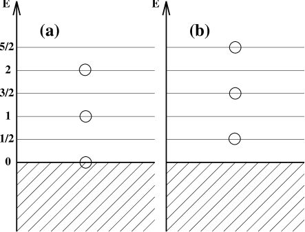
FIG. 1.: Single particle spectrum of a single component Majorana fermion chain; (a) for periodic boundary conditions, (b) for antiperiodic boundary conditions. Energies are give in units of $\pi v_{\rm F}/l$.

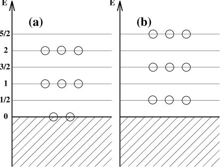
FIG. 2.: Single particle spectrum of a vector Majorana fermion chain; (a) for periodic boundary conditions, (b) for antiperiodic boundary conditions. Energies are give in units of $\pi v_{\rm F}/l$.

FIG. 3.: The separation of the model in the lattice form. The upper chain represents the vector part of the conduction electrons consisting of $\psi_{1}$, $\psi_{2}$, and $\psi_{3}$, while the lower chain represents the scalar part $\psi_{0}$, which decouples from the impurity spin.

FIG. 4.: The picture of the strong-coupling fixed point Hamiltonian in the lattice version. The impurity spin combines one electron at the nearest site to form a singlet bound state, and both the impurity spin and the nearest site of the vector part thus drop out of the problem.

FIG. 5.: Flow diagram for $U=0.001428$, $V=0.01414$ and $V_{\rm a}=V/2$. Solid and dashed lines belong to $j_{\rm tot}=0.5$ and $j_{\rm tot}=1.5$, respectively. The system flows to the non-Fermi liquid fixed point.

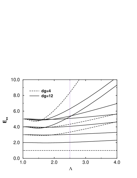
FIG. 6.: $\Lambda$-dependence of the many-body energies $E_{\rm ex}$. The ground state ($E_{\rm ex}\!=\!0$) has four-fold degeneracy. Degeneracies of the excited states plotted here are $dg\!=\!4$ (dashed line) and $dg\!=\!12$ (solid line). The points where the $E_{\rm ex}(\Lambda)$ cross the vertical line at $\Lambda\!=\!2.5$ correspond to the energies obtained from the NRG calculation.

FIG. 7.: Structure of the non-Fermi liquid fixed point. $\tilde{U}$ couples the vector part at site -1 to an additional Majorana-fermion which itself is not coupled to the scalar chain.

FIG. 8.: The interaction vertex function in the first and third order perturbation theory. (a) is the original interaction; (b), (c), and (d) are the third order corrections. (b) and (c) are parquet diagrams, producing the leading logarithmic terms.

FIG. 9.: The total spin susceptibility in the second and fourth order perturbation theory. (a) describes the second order correction, giving rise to a logarithmic term; (b) and (c) are the leading order singular contributions in the fourth order perturbation theory, producing the squared logarithmic corrections.

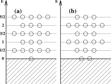
FIG. 10.: Single particle spectra for the two sectors present at the non-Fermi liquid fixed point of the two channel Kondo model. (a) corresponds to sector I and (b) to sector II. The energies are given in units of $\frac{\pi v_{\rm F}}{l}$.

FIG. 11.: Single particle spectra of the compactified models. (a) for PBC in the vector part and APBC in the scalar part (corresponding to $N$ odd) and (b) for APBC in the vector part and PBC in the scalar part (corresponding to $N$ even). The energies are given in units of $\frac{\pi v_{\rm F}}{l}$.

REFERENCES

- [1] P. Coleman, L. Ioffe, and A. M. Tsvelik, Phys. Rev. B 52, 6611 (1995).
- [2] P. Coleman and A. J. Schofield, Phys. Rev. Lett. 75, 2184 (1995).
- [3] A. J. Schofield, Phys. Rev. B 55, 5627 (1997).
- [4] G.-M. Zhang and A. C. Hewson, Phys. Rev. Lett. 76, 2137 (1996); Phys. Rev. B 54, 1169 (1996).
- [5] C. M. Varma, P. B. Littlewood, S. Schmitt-Rink, E. Abrahams, and A. E. Ruckenstein, Phys. Rev. Lett. 63, 1996 (1989).
- [6] N. Andrei and A. Jerez, Phys. Rev. Lett. 74, 4507 (1995).
- [7] P. Nozières, J. Low Temp. Phys. 17, 31 (1974).
- [8] R. Bulla and A.C. Hewson, Z. Phys. B (to be published)
- [9] I. Affleck and A. W. W. Ludwig, Nucl. Phys. B 360, 641 (1991); Phys. Rev. B 48, 7297 (1993).
- [10] J. L. Cardy, Nucl. Phys. B 275, 200 (1986); 324, 581 (1989).
- [11] V. G. Knizhnik and A. B. Zamolodchikov, Nucl. Phys. B 247, 83 (1984).
- [12] P. Ginsparg, in Fields, Strings and Critical Phenomena, Les Houches XLIX, (North Holland, Amsterdam 1990), edited by E. Brèzin and J. Zinn-Justin.
- [13] K. G. Wilson, Rev. Mod. Phys. 47, 773 (1975).
- [14] H. R. Krishna-murthy, J. W. Wilkins and K. G. Wilson, Phys. Rev. B 21, 1003 (1980); 21, 1044 (1980).
- [15] I. Affleck, A. W. W. Ludwig, H.-B. Pang and D. L. Cox, Phys. Rev. B, 45, 7918 (1992).
- [16] I. Antoniadis, C. Bachas, C. Kounnas, and P. Windey, Phys. Lett. 171B, 51 (1986); P. Windey, Comm. Math. Phys. 105, 511 (1986).
- [17] A. C. Hewson (unpublished).
- [18] A. C. Hewson, Phys. Rev. Lett. 70, 4007 (1993); The Kondo Problem to Heavy Fermions (Cambridge Univ. Press, Cambridge, 1993).
- [19] A. C. Hewson, Advances in Physics 43, 543 (1994).
- [20] N. N. Bogoliubov and D. V. Shirkov, Introduction to the Theory of Quantized Fields (Wiley-Interscience, New York 1980), 3rd ed.; L. H. Ryder, Quantum Field Theory (Cambridge Univ. Press, Cambridge 1985).
- [21] D. M. Cragg, P. Lloyd and Ph. Nozières, J. Phys. C, 13, 803 (1980).
- [22] H.-B. Pang, D. L. Cox, Phys. Rev. B, 44, 9454 (1991).
- [23] Jinwu Ye, preprint cond-mat 9612029 (1996).
- [24] Jinwu Ye, preprint cond-mat 9609057 (1996).
- [25] M. Fabrizio, A. O. Gogolin and Ph. Nozières, Phys. Rev. Lett. 74, 4503 (1995).
- [26] S. Bradley, R. Bulla and A. C. Hewson, in preparation (1997).