TPR-96-20

Phys. Rev. A56, 182 (1997)

Periodic orbit theory of a
circular billiard
in homogeneous magnetic fields


J. Blaschke and M. Brack
Institut für Theoretische Physik
Universität Regensburg
93040 Regensburg, Germany

We present a semiclassical description of the level density of a two-dimensional circular quantum dot in a homogeneous magnetic field. We model the total potential (including electron-electron interaction) of the dot containing many electrons by a circular billiard, i.e., a hard-wall potential. Using the extended approach of the Gutzwiller theory developed by Creagh and Littlejohn, we derive an analytic semiclassical trace formula. For its numerical evaluation we use a generalization of the common Gaussian smoothing technique. In strong fields orbit bifurcations, boundary effects (grazing orbits) and diffractive effects (creeping orbits) come into play, and the comparison with the exact quantum-mechanical result shows major deviations. We show that the dominant corrections stem from grazing orbits, the other effects being much less important. We implement the boundary effects, replacing the Maslov index by a quantum-mechanical reflection phase, and obtain a good agreement between the semiclassical and the quantum result for all field strengths. With this description, we are able to explain the main features of the gross-shell structure in terms of just one or two classical periodic orbits.

pacs      03.65.Sq, 73.20.Dx, 73.23.Ps

1 Introduction

The two-dimensional free-electron gas (2DEG) that occurs at the interface of suitably designed semiconductor heterojunctions (see, e.g. [1]) has attracted a lot of interest in the last years. This is partly due to the two dimensionality, which gives rise to new physical effects (such as the quantum Hall effect) and partly to the extremely high mobility of the electrons, which comes from the absence of (scattering) donors or acceptors in the plane of the electron gas. The most attractive feature, however, is the great variability of these systems. With electron-beam lithography additional lateral constraints of the 2DEG down to structures of some 10 $nm$ can be realized. This length is well below the typical phase coherence length and the electron mean free path (in GaAs both of them can be of the order of some $\mu m$), and can even be comparable to the Fermi wavelength of the electrons (typically 40 $nm$ for GaAs), so that in such structures quantum confinement effects play an important role. These systems are therefore accessible on a quantum scale, opening up tremendous new possibilities in device design.

Various approaches heave been used to model the 2DEG with and without additional lateral confinement. Quantum-mechanical calculations tend to be rather involved and even for the simplest systems numerically very demanding. Classical approaches have the severe drawback that they ignore quantum interference effects, and are therefore applicable only if the system dimensions are long compared to the mean free path and the phase coherence length. In the resulting gap of the theoretical description, semiclassical approaches appear very promising. They approximate quantum mechanics in such a way that the quantities involved can be interpreted classically, often in terms of the classical orbits in the system. They combine the advantages of the classical description, especially its limited numerical demands, with the ability to reproduce quantum-mechanical interference effects. This makes semiclassical methods a very attractive tool for mesoscopic systems, i.e., systems with dimensions comparable to the phase coherence length and the mean free path. One of the most striking successes in recent years has been the explanation of conductance oscillations in superlattices, the Weiss oscillations [2].

In this paper, we consider the level density of a 2DEG confined by external electric fields to a circular domain, with an additional homogeneous magnetic field perpendicular to the plane of the 2DEG. When this quantum dot contains many electrons, the effective single-particle potential (i.e., the Kohn-Sham potential in the language of density functional theory, which contains the electron-electron interaction in the local density approximation) is Wood-Saxon-like, with a flat region in the interior and a rather steep surface. The level density is not too sensitive to details of the potential edge, so that a circular disk with infinite reflecting walls, i.e., a circular billiard, is a realistic model.

The level density itself is hard to access experimentally, but it enters in many observable quantities. Persson et al. [5], for example, consider a quantum dot that is connected by two point contacts to the surrounding 2DEG. They propose an approximation in which the conductivity of this system in weak external magnetic fields is proportional to the level density of the dot at the Fermi energy. Their measurements on a circular dot with about 1000 – 1500 electrons in a homogeneous magnetic field show characteristic conductance oscillations that could be well explained qualitatively in a perturbative approach by Reimann et al. [7]. They reproduce the oscillations in a simple and intuitive way by a few classical periodic orbits of the system and the flux enclosed by them. Because of its perturbative nature, this description only holds in weak fields. Another example where the level density enters observable quantities is the magnetization [8, 9].

For the interpretation of experiments on circular quantum dots, a semiclassical approximation of the level density with arbitrary field strength is desirable. Such a description in terms of classical orbits is also of theoretical interest. In the absence of a magnetic field the classical orbits consist of straight paths bouncing at the boundary (see Fig. 2). They have a one-dimensional degeneracy corresponding to the rotational symmetry of the system. In very strong fields, the confinement is negligible and the level density is dominated by the quantization of a free-electron gas, leading quantum mechanically to the Landau levels and described semiclassically by closed cyclotron orbits. These orbits do not touch the boundary and have a two-dimensional translational degeneracy. A unified semiclassical description thus has to include the transition between these two limiting cases, which includes changes of the topology and the degeneracy of the classical orbits. Treating these is of conceptual interest since both effects are well known to lead to divergences in semiclassical theories.

We conclude this Introduction with a short outline of the paper. As a reference, we first present in Sec. 2 the quantum-mechanical solution for the circular billiard in homogeneous magnetic fields. Section 3 gives a short introduction to semiclassical methods, and in Sec. 4 we derive a semiclassical trace formula of the disk. We then compare its results to the quantum-mechanical ones for various field strengths. The agreement is good for very weak and for very strong fields, but the semiclassical approach rather appears to fail in the intermediate regime. The deviations are due to bifurcations of classical orbits, to diffraction effects, and to boundary effects. The latter give the largest contributions, and in Sec. 5 we develop a simple approximation to include these effects in the trace formula. This corrected trace formula gives satisfactory results for all magnetic field strengths, and we give an intuitive interpretation of the the level density in the various $B$-field regimes. The paper closes with a summary of the results and an outlook to further investigations.

2 The quantum-mechanical solution

In the following, we will use normalized energies $\widetilde{E}$ in units of $\hbar^{2}/2mR^{2}$ and normalized magnetic fields $\widetilde{B}$ in units of $\hbar/eR^{2}$, where $R$ is the disk radius. In these units, we have $\sqrt{\widetilde{E}}=kR$ and with the classical cyclotron radius $R_{c}=\hbar k/eB$, we get $R_{c}/R=kR/\widetilde{B}$.

The exact quantum-mechanical solution for the circular billiard in homogeneous magnetic fields was presented by Geerinckx [10] and, using a different approach, by Klama and Rößler [11]. The eigenenergies are given by the zeros of the confluent hypergeometric function ${}_{1}F_{1}$ as

$$\widetilde{E}_{nl}=2\widetilde{B}\cdot\left(\alpha_{nl}+\frac{1+|l|}{2}+\frac{1}{2}\right)\quad,$$ (1)

where

$${}_{1}F_{1}\left(-\alpha_{nl};1+|l|;\frac{\widetilde{B}}{2}\right)=0\quad.$$ (2)

Here $n>0$ denotes the radial and $l$ the angular-momentum quantum number. The zeros of ${}_{1}F_{1}$ were determined numerically — which is conceptually easy but requires a lot of numerical work. Figure 1 shows the well-known dependence of the eigenvalues $\widetilde{E}_{nl}$ on $\widetilde{B}$. One clearly sees how with increasing magnetic field the different states condense into the Landau levels (dashed lines).

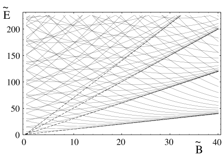
Figure 1: The quantum-mechanical eigenenergies of the circular billiard in dependence of the magnetic field. The dashed lines correspond to the four lowest Landau levels.

3 Semiclassical methods

For semiclassical approximations, a broad variety of methods is at hand. Some of them approximate directly the quantum-mechanical eigenvalues [12, 13], whereas others describe the level density $g(E)$. For this purpose, $g(E)$ is usually split up into a smooth part $\tilde{g}(E)$, the (extended) Thomas-Fermi level density, and an oscillating part $\delta g$:

$$g(E)=\tilde{g}(E)+\delta g(E)\quad.$$ (3)

The latter can be expressed in terms of the periodic orbits of the corresponding classical system, which is therefore called periodic orbit theory (POT). Such relations have been established by various approaches [14, 15, 16, 17, 18], usually resulting in so-called trace formulae of the form

$$\delta g(E)=\frac{1}{\pi\hbar}\sum_{\Gamma}A_{\Gamma}\sin\left(\frac{S_{\Gamma}(E)}{\hbar}-\sigma_{\Gamma}\frac{\pi}{2}+\frac{\pi}{4}\right)\quad.$$ (4)

Here $\Gamma$ labels all classical periodic orbits of the system. Each orbit contributes to the level density via an oscillating term that depends on the classical action $S_{\Gamma}$ along the orbit and on the Maslov index $\sigma_{\Gamma}$ depending on the orbit’s topology. The amplitude $A_{\Gamma}$ is a slowly varying function of energy, determined by classical properties of the orbit such as its degeneracy and its stability. All semiclassical approaches have their individual merits and drawbacks [19], and it is interesting to note that for the simple integrable case of the circular billiard without magnetic field, all applicable methods result in the same trace formula [20, 21, 22], which furthermore reproduces exactly [22] the EBK spectrum. Applying a homogeneous magnetic field, the system remains integrable, with the energy and the $z$ component of the conjugate angular momentum as constants of the motion. In weak fields, this system was treated using a perturbative approach by Bogachek and Gogadze [21], Ullmo et al. [8], and by Reimann et al. [7]. We have chosen the trace formula of Creagh and Littlejohn [18] as a starting point for the description in arbitrarily strong fields.

4 Trace formula for the circular billiard

The trace formula of Creagh and Littlejohn [18] is well suited for the semiclassical description of the circular billiard, as it can deal with continuous symmetries. The main idea of their approach is the separation into a symmetry-free system treated by usual semiclassical techniques and the symmetry, which is used to integrate over the orbit families. The structure of the trace formula (4) remains essentially unchanged by this procedure, but the definition of $A$ is different, reflecting the different classical structure of the dynamics. For the details we refer to the original publication [18]. In order to calculate the level density with this trace formula, we have to classify the periodic orbits and calculate their actions, amplitudes, and Maslov indices. These steps are presented in the following subsections.

4.1 Classification of the periodic orbits

The complete classification of the periodic orbits of our system is straightforward. Let us first consider the case without magnetic field. In a circular billiard, the periodic orbits (PO) are identical to those in a three-dimensional spherical cavity, whose complete classification has been given by Balian and Bloch [15]. All orbits have a one-dimensional degeneracy corresponding to the rotational symmetry of the system. Each family of degenerate orbits with a given action (or length) can be represented by a regular polygon. The first few polygons are shown in Fig. 2.

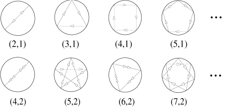
Figure 2: The classical periodical orbits of the circular billiard in the absence of a magnetic field are the regular polygons. They can be classified with $(v,w)$, where $v$ is the number of corners and $w$ indicates how often the trajectory winds round the center of the disk.

These orbit families are classified [15] by $\beta=(v,w)$, where $v$ denotes the number of corners (vertices), and $w$ is the winding number, i.e., it counts how often an orbit winds around the center. With $v\geq 2w>2$, $\beta=(v,w)$ uniquely describes all families of POs of the system in the absence of a magnetic field. Because of the time-reversal symmetry, all orbits except the diameter ($v=2w)$ have an additional discrete twofold degeneracy, which has to be accounted for in the trace formula.

Switching on the magnetic field causes the classical trajectories to bend, with the direction of the curvature depending on the direction of motion with respect to the magnetic field. This entails a breaking of time-reversal symmetry. For weak fields, the orbits can still be classified by $\beta$ if an additional index ($\pm$) is introduced. This situation is shown in the upper row of diagrams in Fig. 3 for the orbit $\beta=(4,1)$. Up to a field strength where the classical cyclotron radius $R_{c}$ equals the disk radius $R$, henceforth referred to as the weak-field regime, the orbits do not change their topology and the classification $\beta^{\pm}$ holds. For the strong-field regime with $\widetilde{B}>kR$, the structure of the POs is different. This situation is shown in the second row of diagrams in Fig. 3. The $\beta^{-}$ orbits change their shape continuously over the point $R_{c}=R$, but the $\beta^{+}$ orbits change their topology abruptly. However, since there is a one-to-one correspondence between orbits for $R_{c}\mbox{\raisebox{2.15277pt}[-2.15277pt][0.0pt]{$\scriptstyle>$} \raisebox{-8.61108pt}[0.0pt][-8.61108pt]{\Large\char 126\relax}}R$ and for $R_{c}\mbox{\raisebox{2.15277pt}[-2.15277pt][0.0pt]{$\scriptstyle<$} \raisebox{-8.61108pt}[0.0pt][-8.61108pt]{\Large\char 126\relax}}R$, $\beta^{\pm}$ still gives a complete classification of all bouncing orbits, i.e., of orbits that are reflected at the boundary. For $R_{c}<R$, there are additional cyclotron orbits that do not touch the boundary at all. They have to be included separately in the sum over all orbits in the trace formula.

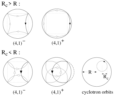
Figure 3: A magnetic field breaks the time-reversal symmetry, so that the orbits are no longer independent of the direction of motion. Introducing an additional index $\pm$, the orbits can be classified by $(v,w)^{\pm}$, both in weak ($R_{c}>R$) and in strong ($R_{c}<R$) fields. For strong fields, there occurs an additional family of orbits that do not touch the boundary, the cyclotron orbits.

At field strengths where $R_{c}\leq R\sin(\pi w/v)$, the $(v,w)^{\pm}$ orbits no longer exist (see Fig. 4). They vanish pairwise, which is the simplest case of an orbit bifurcation. This imposes an additional restriction on the sum over $(v,w)$. Including this, we now have a complete classification of all periodic orbits in the circular billiard at arbitrary field strengths.

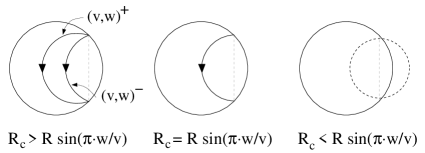
Figure 4: At a field strength where $R_{c}=R\sin(\pi\;w/v)$, the orbits $(v,w)^{\pm}$ vanish pairwise.

4.2 The bouncing orbits

The action of a closed orbit in a magnetic field can be written as the sum of the kinetic part and the magnetic flux enclosed by the orbit

$$S_{\beta}=\int p\,\mbox{d}q=\hbar kL_{\beta}-eBF_{\beta}\qquad.$$ (5)

The geometrical lengths $L_{\beta}$ and the enclosed areas $F_{\beta}$ of the periodic orbits discussed above (correctly counting those areas that are enclosed several times, cf. Fig. 5) can be calculated by elementary geometry. In terms of the geometrical quantities $R_{c},R,\gamma$ and $\Theta$, explained in Fig. 6, we obtain

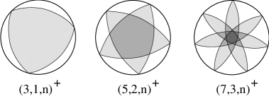
Figure 5: Calculating the magnetic flux enclosed by an orbit, the multiply enclosed areas (darker gray) have to be correctly accounted for.

$$S_{\beta}(E) = v\hbar kR_{c}\eta\quad,$$ (6)

$$\eta = \left\{{\begin{array}[]{rccccp{5mm}}\gamma&+&\frac{\sin 2\gamma}{2}&-&\left(\frac{R}{R_{c}}\right)^{2}\frac{\sin 2\Theta}{2}&\\ \lx@intercol\hfil\rule{0.0pt}{10.76385pt}\mbox{for }(\beta^{+},R_{c}\geq R)\lx@intercol\\ \rule{0.0pt}{19.37494pt}\pi-\gamma&-&\frac{\sin 2\gamma}{2}&+&\left(\frac{R}{R_{c}}\right)^{2}\frac{\sin 2\Theta}{2}&\\ \lx@intercol\hfil\rule{0.0pt}{10.76385pt}\mbox{for }(\beta^{+},R_{c}\leq R)\lx@intercol\\ \rule{0.0pt}{19.37494pt}\gamma&+&\frac{\sin 2\gamma}{2}&+&\left(\frac{R}{R_{c}}\right)^{2}\frac{\sin 2\Theta}{2}&\\ \lx@intercol\hfil\rule{0.0pt}{10.76385pt}\mbox{for }(\beta^{-})\lx@intercol\end{array}}\right.\quad.$$ (13)

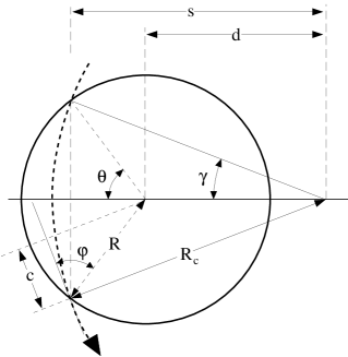
Figure 6: The actions and amplitudes of the classical periodical orbits can be expressed purely in terms of the geometrical quantities shown here.

According to the trace formula [18], the orbit amplitudes are composed of an integral over the symmetry group, which for the rotational $U(1)$ symmetry of the disk just gives $2\pi/v$, of the period of the orbit $L/\hbar k$, and of the Jacobian resulting from the symmetry reduction $\mbox{d}L/\mbox{d}\Psi$, where $\Psi=-2n\Theta$. All these quantities can be calculated analytically, resulting in

$$A_{\beta} = \frac{1}{E_{0}}\frac{1}{\sqrt{Rk\pi}}\frac{1}{\sqrt{v}}\frac{R_{c}}{R}\sqrt{\frac{cd}{sR}}\;\xi_{\beta}\quad,$$ (14)

$$\quad\xi_{\beta} = \left\{\begin{array}[]{ll}\pi-\gamma&\mbox{for }(\beta^{+},R_{c}<R)\\ \gamma&\mbox{otherwise}\end{array}\right.\;,$$ (17)

where $c,d,$ and $s$ are the geometrical lengths sketched in Fig. 6. The connection of these geometrical quantities to the classification parameter $\beta^{\pm}$ and the cyclotron radius $R_{c}$ is given in Appendix A.

4.3 Cyclotron orbits

For magnetic fields stronger than $\widetilde{B}=kR$, the classical cyclotron radius $R_{c}$ is smaller than the disk radius $R$. This gives rise to a new class of periodic orbits, the cyclotron orbits, which do not touch the boundary at all (see Fig. 3). They form translationally degenerate families, whereas the bouncing orbits $(v,w)^{\pm}$ considered above are degenerate with respect to rotations. For the translational case, the symmetry reduction can be performed directly, without need of the general procedure of Creagh and Littlejohn. We transform the phase-space coordinates according to

$$\pi_{x}:=\frac{1}{\sqrt{|eB|}}\left(p_{x}+\frac{eB}{2}y\right); \Pi_{x}:=\pi_{y}+\sqrt{|eB|}\;x$$

$$\pi_{y}:=\frac{1}{\sqrt{|eB|}}\left(p_{y}-\frac{eB}{2}x\right); \Pi_{y}:=\pi_{x}-\sqrt{|eB|}\;y\;.$$

Apart from a factor $\sqrt{|eB|}$, $(\pi_{x},\pi_{y})$ are the coordinates of the motion relative to the center of gyration $(\Pi_{x},\Pi_{y})$, as illustrated in Fig. 7.

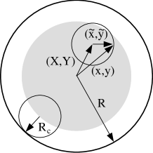
Figure 7: The motion of a charged particle in a homogeneous magnetic field can be expressed in the coordinates of the relative motion $(\tilde{x},\tilde{y})=|eB|^{-1/2}(-\pi_{y},\pi_{x})$ and the coordinates of the center of gyration $(X,Y)=|eB|^{-1/2}(\Pi_{x},-\Pi_{y})$. The Hamiltonian is independent of $(\Pi_{x},\Pi_{y})$; all orbits with the center $(X,Y)$ in the gray shaded area are degenerate.

In these coordinates the Hamiltonian reads

$$H=\frac{eB}{2m}(\pi_{x}^{2}+\pi_{y}^{2})\quad.$$ (19)

As expected, $H$ does not depend on the coordinates of the center of gyration. $\Pi_{x}$ and $\Pi_{y}$ are canonically conjugate variables, since $[\Pi_{x},\Pi_{y}]=i\hbar$. Because the relative and the center-of-gyration coordinates commute, i.e., $[\Pi_{x},\pi_{x}]=[\Pi_{x},\pi_{y}]=[\Pi_{y},\pi_{x}]=[\Pi_{y},\pi_{y}]=0$, the degeneracy of a cyclotron orbit is simply the phase-space volume $V$ accessible for $(\Pi_{x},\Pi_{y})$, which can be directly read off Fig. 7 (shaded area). We therefore get for the degeneracy

$$N=\frac{V}{2\pi\hbar}=\frac{\tilde{B}}{2}\left(1-\frac{R_{c}}{R}\right)^{2}\qquad.$$ (20)

Now, the Hamiltonian Eq. (19) is identical to that of a one-dimensional harmonic oscillator. Using its analytically known trace formula, the contribution of the cyclotron orbits to the oscillating part of the level density is given by

$$\delta g^{c}=\frac{1}{2E_{0}}\left(1-\frac{R_{c}}{R}\right)^{2}\sum_{n=1}^{\infty}\cos(nk\pi R_{c}-n\pi)\quad.$$ (21)

Here $n$ is the winding number around the center of gyration. Note that the frequency is again determined by the classical action along the orbit, which in this case is

$$S=n\cdot\hbar k\cdot\pi R_{c}\qquad.$$ (22)

Note that here exactly half of the kinetic contribution to the action is canceled by the flux term.

4.4 Additional phases

For a discussion of the additional phases in the trace formula (4) we refer to Sec. 5.1. There we find that the Maslov index for bouncing orbits is $\sigma=3v$, and for the cyclotron orbits it is $\sigma=2$. According to [18, 24], we have an additional phase of $\delta\;\pi/2$ stemming from the symmetry reduction. $\delta$ is found to be

$$\delta=\left\{\begin{array}[]{c@{\hspace{5mm}}l}0\hfil\hskip 14.22636pt&\mbox{for }(\beta^{+},R_{c}<R)\\ 1\hfil\hskip 14.22636pt&\mbox{otherwise.}\end{array}\right.\qquad.$$ (23)

We have now analytic formulas for all quantities of the trace formula. The numerical evaluation of this semiclassical level density will be performed in Secs. 4.6 and 4.7.

4.5 The shell structure

In an experiment, the observed levels are always broadened due to temperature, life-time, or impurity effects. In most systems the levels are not approximately equally spaced, but occur in bunches, the so-called shells, which are separated by relatively wide energy gaps. Smoothing the level density over a width larger than the typical level spacing, but smaller than the distance of the bunches, reveals the (gross-) shell structure of the system. It contains in many cases the dominating quantum effects. This folding procedure can easily be implemented in the semiclassical trace formula. For pure billiard systems, i.e., systems where $S=kL$ with $L$ independent of $k$, a Gaussian folding of the level density is equivalent to the multiplication of the orbit amplitudes in the trace formula with a Gaussian with reciprocal width. In Appendix B we give a more general form of this relation, which is not restricted to pure billiard systems and to Gaussian smoothing, but can deal with general systems and arbitrary smoothing functions. We will in the following use this generalized approach, as in finite magnetic fields we no longer have a pure billiard system. As this is a more technical point, we leave the discussion for Appendix B. There we also give detailed information about the numerical evaluation scheme and the smoothing function used. The latter is in the following characterized by a parameter $\tilde{\gamma}$, which corresponds to the variance of a Gaussian $\exp[-1/2\left(kR/\tilde{\gamma}\right)^{2}]$ with the same half-width.

The additional factor in the amplitudes stemming from the smoothing strongly suppresses the longer periodic orbits, so that usually only a few of them (2 - 10) contribute to the gross-shell structure. This makes the POT a very convenient tool for the calculation of this quantity. The quantum-mechanical approach is in some sense complementary to the semiclassical one. It first gives the single eigenvalues, of which many have to be known to calculate the shell structure. On the other hand, a full semiclassical quantization, i.e., resolving the level density down to the single eigenenergies, involves in general an exponentially increasing number of orbits and thus is a very demanding task. Here we are mainly interested in the semiclassical calculation of the gross-shell structure, for which only a few of the shortest and most degenerate periodic orbits are required. We will, nevertheless, also try to go for a full quantization — mainly to verify the quality of our semiclassical approximation.

4.6 Results in the weak-field regime

In the previous sections we have derived an analytical trace formula for the circular billiard in homogeneous magnetic fields of arbitrary strength. Presently we shall discuss the resulting level densities as a function of energy and magnetic field. Let us start with weak fields ($R_{c}>R$), for which the topology of the classical periodic orbits is the same as in the absence of a magnetic field (see Sect. 4.1), so that we expect the semiclassical approach to be of the same quality as for zero field. The high-field regime, where we expect new effects to arise, will be the topic of the next section.

The case of the circular billiard in small homogeneous magnetic fields has already been treated by Bogachek and Gogadze [21] and by Reimann et al. [7] using a perturbative approach for weak fields. Replacing the amplitudes of Eq. (14) by their asymptotic values for $\widetilde{B}\to 0$ and expanding the actions of Eq. (6) up to first order in $\widetilde{B}$ reproduces, indeed, their results.

In Fig. 8 the semiclassical level density obtained with ${\widetilde{\gamma}}=0.35$ (solid line) is plotted against the equivalently smoothed quantum result (dashed) for various values of $\widetilde{B}$.

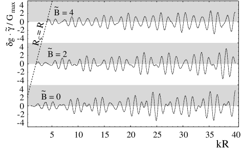
Figure 8: The semiclassical level density of the disk billiard (solid line) matches perfectly the equivalently smoothed quantum-mechanical result (dashed, and well hidden under the solid line). The smoothing width is $\tilde{\gamma}=0.35$.

The agreement is almost perfect — just as it is in the zero-field case, which has been extensively discussed by Reimann et al. [25]. Note that the calculation requires over 850 numerically determined eigenvalues for the quantum-mechanical calculation (which then have to be smoothed), whereas the semiclassical calculation is analytical and just requires the most important orbits (the diameter and the two triangle, square, pentagon and hexagon orbits).

Since we have a classification of all periodic orbits and analytic expressions for their actions and amplitudes, we can attempt a full semiclassical quantization by summing up sufficiently many of them. The result is shown in Fig. 9, where we display the total level density $g=\tilde{g}+\delta g$, averaged over a width ${\widetilde{\gamma}}=0.025$, which is smaller than the typical level spacing. As Tanaka has shown in [9], the smooth part of the level density of the circular billiard does not depend on the magnetic field to leading order in $\hbar$. We use the Thomas-Fermi level density for zero field, which is identical to the familiar Weyl expansion [26]

$$\tilde{g}(k)=\frac{1}{4E_{0}}\left(1-\frac{1}{kR}\right)\quad.$$ (24)

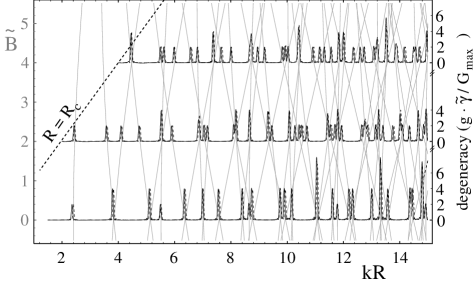
Figure 9: The semiclassical level density (solid) for a smoothing width $\tilde{\gamma}=0.025$, which is small enough to resolve the single eigenenergies (“full quantization”). One can hardly distinguish this from the equivalently smoothed quantum-mechanical result (dashed line underneath). The positions of the quantum-mechanical eigenvalues in dependence of $\tilde{B}$ are indicated by the gray lines.

Both the semiclassical level density (solid) and the corresponding quantum-mechanical one (dashed) in Fig. 9 exhibit clearly separated peaks whose heights give the degeneracies of the individual levels. The two lines can hardly be distinguished, thus the semiclassical approach gives almost perfect results even in this extreme case of full quantization.

4.7 Results in the strong-field regime

Figure 10 is the strong-field equivalent of Fig. 8. It displays again the semiclassical (solid) and the quantum-mechanical (dashed) level densities, obtained with an equivalent averaging width $\widetilde{\gamma}$ = 0.35.

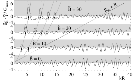
Figure 10: The semiclassical level density ($\tilde{\gamma}=0.35$) of the disk billiard (solid) compared to the equivalently smoothed quantum-mechanical result (dashed). The gray lines and the arrows indicate the positions of the first four Landau levels. For strong fields ($R_{c}<R$), the agreement between the semiclassical and the quantum-mechanical results is not satisfactory.

The agreement for small fields ($R_{c}<R$) is good, as already shown in Sec. 4.6. For stronger fields, the positions of the Landau levels (gray lines in Fig. 10) are well reproduced, but their degeneracies are overestimated in the semiclassical approximation.

Figure 11 corresponds to Fig. 9 and displays the full quantization of the system.

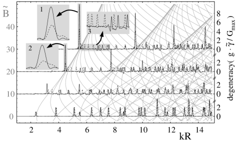
Figure 11: The semiclassical level density resolved up to the single eigenenergies (solid) compared to the equivalently smoothed quantum-mechanical levels (dashed). The gray lines indicate the positions of the eigenenergies as functions of $\tilde{B}$. For strong fields ($R_{c}<R$) the agreement between semiclassical and quantum-mechanical calculation is bad. Note especially the large discrepancies in the degeneracies of the Landau levels, and the completely missing states slightly above the Landau levels (see insets).

The semiclassical approach is seen to fail for stronger fields. As already mentioned, this is due to the neglect of various effects. First, there are orbit bifurcations where classical orbits vanish pairwise with increasing magnetic field (see Figs. 4, 17 and 18). The change of the topology of the $\beta^{+}$ orbits and the occurrence of cyclotron orbits are also bifurcation effects. Those are known to lead to divergences in the trace formula. Second, we have neglected boundary effects from grazing orbits and diffraction effects, which could be implemented in the trace formula by considering creeping orbits. A closer look at Fig. 11 gives some hints as to which of these effects dominate. The two most striking observations are as follows: (1) The trace formula reproduces well the positions of the Landau levels, but it overestimates the degeneracies of these states. The error becomes smaller with increasing field strength (see insets in Fig. 11). (2) The levels that have energies slightly above the Landau levels are completely missed by the semiclassical approach. These two observations suggest that it is a boundary effect that causes the discrepancies. A simple hand-waving argument might be useful to illustrate the effect. Quantum mechanically, a particle moving on a cyclotron orbit will feel the boundary even if classically not touching it. Particles on cyclotron orbits close to the boundary thus feel an additional confinement. This restriction to a smaller volume will lead to a higher energy. In this picture, not all the cyclotron orbits are degenerate. The orbits close to the boundary will no longer have the energy of the Landau level, but a slightly higher one. This is exactly what would correct the observed defects of the semiclassical approximation. In the next section we will present a simple way to incorporate this boundary effect in the trace formula.

5 Boundary corrections to the
trace formula

The observations of Sec. 4.7 suggest that boundary effects are responsible for the failure of the semiclassical approximation in strong fields. The only place where boundary properties enter the standard trace formula is the Maslov index. We therefore propose here to replace the Maslov index by a more sophisticated quantity, which includes some quantum effects. Before doing this, let us give a brief summary of the origin of the Maslov index.

5.1 The Maslov index

The origin of the Maslov index can most easily be understood in the one-dimensional case. Semiclassically, one approximates the wave functions to lowest order by plane waves with the local wave number $k(x)=\sqrt{2m[E-V(x)]}$. This approximation obviously breaks down at the classical turning points where $E=V(x)$ and the wavelength diverges. Expanding the wave function around the classical turning points and matching the solutions to the plane-wave solutions far from the turning points leads to additional phases in the semiclassical quantization [12]. In the limit $\hbar\to 0$ these are independent of the detailed shape of the potential. Each reflection at a soft turning point gives a phase of $-\pi/2$, whereas each reflection at an infinitely steep wall gives a phase of $-\pi$. Writing this phase as $-\sigma\;\pi/2$, one usually calls $\sigma$ the Maslov index.

In the case of the circular disk, the Maslov index can be obtained simply by counting the classical turning points of the one-dimensional effective potential in the radial variable $r$. For skipping orbits, the Maslov index per bounce is 3, including one soft reflection at the centrifugal barrier and one hard-wall reflection. For the cyclotron orbits, the effective potential is a one-dimensional harmonic oscillator (see Sec. 4.3) with two soft turning points, and thus their Maslov index per period is 2.

5.2 Reflection phases

For finite $\hbar$ the additional phase stemming from classical turning points will depend on the shape of the potential. Let us consider a cyclotron orbit at a distance $x_{W}$ to the billiard boundary. Neglecting the curvature of the boundary (which corresponds to the strong-field limit), we can reduce the motion in the presence of the wall to an effective 1D motion just as in the unbounded case presented in Sec. 4.3. This is shown in Fig. 12.

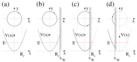
Figure 12: The planar cyclotron orbit is equivalent to the motion in a one-dimensional harmonic oscillator (a). Neglecting its curvature, the billiard boundary can be implemented in the effective one-dimensional motion (b)-(d).

The upper row of diagrams shows the 2D motion, the lower row gives the reduction to the one-dimensional motion in an effective potential. Figure 12 (a) shows the unbounded case, in (b) the orbit is near the boundary, and (c,d) illustrate skipping orbits.

A particle in the potential sketched in Fig. 12b is classically not influenced by the additional wall, since it will never touch it. Quantum mechanically, however, the wave function enters the classically forbidden region and thus feels the boundary even for $x_{W}>R_{c}$. This leads to a smooth transition of the quantum-mechanical reflection phase $\varphi_{R}$ over the point $x_{W}=R_{c}$, whereas the semiclassical Maslov phase is discontinuous at this point; as we have just seen in Sec. 5.1 above, it is $-\pi$ for $x_{W}>R_{c}$ and $-3/2\pi$ for $x_{W}<R_{c}$. Our way to implement these quantum effects at the boundary in the semiclassical trace formula is therefore to replace the Maslov index by the quantum-mechanical reflection phase $\varphi_{R}$ of the corresponding one-dimensional motion. This smooth version of the Maslov phase will also remove the former clear separation between cyclotron orbits and skipping orbits. These two limiting cases are now continuously linked, with $\varphi_{R}$ ranging between $-\pi$ and $-3/2\pi$. We will refer to the orbits in the transition region, which are close to the boundary within $\hbar$, as to the grazing orbits.

The calculation of the reflection phases is in this approximation reduced to the problem of the one-dimensional harmonic oscillator in an additional square-well potential. This system was approached by Isihara and Ebina [27] who used local expansions in terms of Airy functions. We use a different approach and integrate the quantum-mechanical problem numerically. From the solutions we calculate the reflection phases $\varphi_{R}$, which is displayed in Fig. 13.

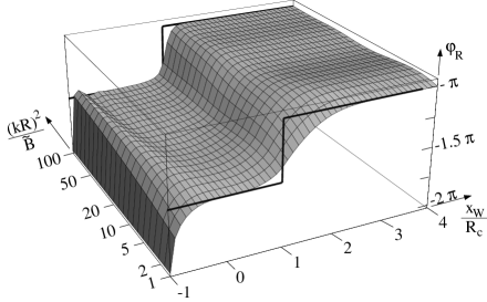
Figure 13: The reflection phase $\varphi_{R}$ in dependence of the distance of the center of gyration from the boundary $x_{W}$. The transition from $x_{W}<1$ to $x_{W}>1$ is continuous and gets sharper for increasing $(kR)^{2}/\widetilde{B}$. In the limit $(kR)^{2}/\widetilde{B}\to\infty$, which corresponds to the semiclassical limit $\hbar\to 0$, the Maslov phase (thick line) is recovered.

As expected, they show a smooth transition from $-\pi$ at $x_{W}\gg R_{c}$ to $-3/2\pi$ at $x_{W}\ll R_{c}$. The transition gets sharper if $(kR)^{2}/\widetilde{B}$ increases. For $(kR)^{2}/\tilde{B}\to\infty$, which corresponds to the semiclassical limit $\hbar\to 0$, the standard Maslov phase (thick line) is reproduced. Quantum corrections are seen to have the greatest influence on the grazing orbits $(x_{W}\approx R_{c})$ and on orbits with $x_{W}\mbox{\raisebox{2.15277pt}[-2.15277pt][0.0pt]{$\scriptstyle>$} \raisebox{-8.61108pt}[0.0pt][-8.61108pt]{\Large\char 126\relax}}-R_{c}$. These are known as the whispering gallery orbits, as they move in a narrow region along the boundary.

5.3 Comparison to the
quantum-mechanical result

Figures 14 and  15 show the coarse-grained level density and the full quantization of the spectrum, respectively, both calculated with the reflection phases of Sect. 5.2.

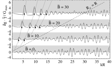
Figure 14: The semiclassical coarse-grained level density of the disk calculated with reflection phases (solid) compared to the equivalently smoothed quantum-mechanical result (dashed). The gray lines and the arrows indicate the positions of the lowest Landau levels. The agreement is considerably better than with the use of the Maslov indices as displayed in Fig. 10.

Figure 15: The semiclassical level density with corrected reflection phases resolved up to the single eigenenergies of the billiard (solid) compared to the equivalently smoothed quantum-mechanical result (dashed). The gray lines indicate the positions of the eigenenergies in dependence of $\tilde{B}$. The agreement is much better than in the case of the Maslov indices in Fig. 11. The degeneracies of the Landau levels are correctly reproduced, only the levels that are close to condensing on the Landau levels show deviations (insets).

A comparison with the corresponding diagrams in Figs. 10 and 11, which display the result obtained with the standard Maslov indices, immediately shows that the situation is drastically improved when using reflection phases. The coarse-grained level density now is good at all magnetic field strengths. The full quantization displayed in Fig. 15 is not perfect, but the most striking error in standard POT, giving the wrong degeneracies of the Landau levels, is now corrected. This is displayed in detail in the insets 1 and 2 in Figs. 11 and 15, respectively. The single states between the Landau levels, however, are still not reproduced correctly. This is due to our simple approximation, which only includes boundary effects via the reflection phase. The classical orbits are not changed, so that in our approximation the center of gyration of the cyclotron orbits ($x_{W}>R_{c}$) is fixed, whereas for bouncing orbits ($x_{W}<R_{c}$) it moves around the disk. Modeling the expected smooth transition from $x_{W}>R_{c}$ to $x_{W}<R_{c}$ semiclassically would require including diffractive orbits that we have neglected here. The resulting error can be understood as follows: a generic two-dimensional system has two quantum numbers, thus requiring two semiclassical quantization condition. The free 2D electron gas in a homogeneous magnetic field has an additional dynamical symmetry and only one quantum number (labeling the Landau level). This additional symmetry is broken by the presence of a curved boundary. This implies that the semiclassical description in terms of cyclotron orbits near the boundary misses one quantization condition, which is hidden in the broken dynamical symmetry. Therefore these orbits give rise to a continuous semiclassical (sub) spectrum. Bouncing orbits, however, have the correct symmetry and lead to a discrete subspectrum. This transition can be seen in Fig. 15. On the low-energy side of inset 3, the semiclassical level density shows a continuous spectrum stemming from the grazing orbits, whereas the quantum-mechanical result gives quantized levels. This error affects mainly the fully quantized spectrum; the influence on the gross-shell structure is negligible.

Figure 16 shows once again the semiclassical level density calculated with reflection phases, now in the whole range from zero field to full Landau quantization (solid). The comparison with the exact quantum result (dashed) shows that the semiclassical approximation is in fact valid for arbitrarily strong fields. Small deviations occur only at the bifurcation points of the dominating orbits. As already mentioned, we did not include the effects of the bifurcations in our calculation. The resulting errors are much smaller than the effect of the reflection phase, and they are seen to be more important for the gross-shell structure than for the full quantization.

5.4 Semiclassical interpretation of the
shell structure

In Sec. 5.3 we have shown that the semiclassical approximation for the level density is valid for arbitrarily strong fields. It reproduces the exact quantum-mechanical result with a remarkably reduced numerical effort. For the quantum-mechanical calculation shown in Fig. 16 about 2500 eigenvalues had to be calculated and numerically smoothed for each value of $\widetilde{B}$, whereas the semiclassical result is obtained summing the contributions of just 20 orbits. The most attractive feature of the semiclassical approximation, however, is the simple, intuitive picture it gives. Let us now exploit this to explain the behavior of the shell structure of the disk billiard in terms of classical quantities.

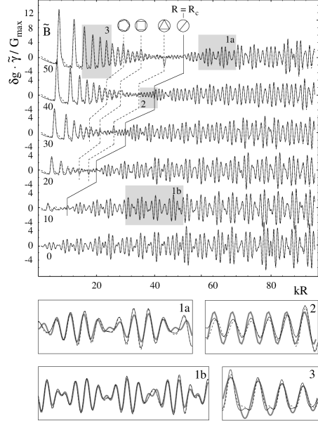
Figure 16: The semiclassical coarse-grained level density of the disk billiard with corrected reflection phases (black) compared to the equivalently smoothed quantum-mechanical result (gray). The agreement is acceptable in the whole range of energies, disk radii, and magnetic fields. The vertical lines indicate the bifurcation points of the most important orbits. The shaded regions are enlarged in the figures below. There the thick lines show the interpretation of the level density as given in the text.

According to the trace formula Eq. (4), each periodic orbit $\beta$ contributes an oscillating term to $\delta g$. Its frequency is determined by the classical action $S_{\beta}$ along this path, which can be locally approximated by

$$S_{\beta}(k)=S_{\beta}(k_{0})+\hbar G_{\beta}(k)\;(k-k_{0})\quad,$$ (25)

with the quasiperiod $\hbar G$. As shown in Appendix B, for systems with constant absolute velocity along an orbit $G$ is the geometrical orbit length. The amplitudes of the oscillating terms are $A_{\beta}F(G_{\beta})$, where $F$ is the window function that depends on the desired smoothing of the level density (see Appendix B). Before we interpret the contributions of the various orbits to $\delta g$, let us discuss the behavior of $G_{\beta}$ and $A_{\beta}$.
Figure 17 shows the dependence of $G$ on the ratio $R_{c}/R$.

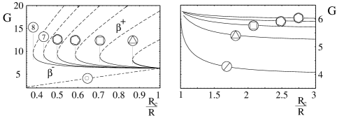
Figure 17: The quasiperiods $G$ of the most important orbits in dependence of $R_{c}/R$. For $R_{c}>R$, $G$ is independent of the index $\pm$. The orbit bifurcation points in strong fields (vertical lines) can be clearly seen.

Note that for $R_{c}>R$ (see right diagram of Fig. 17) $G$ is independent of the direction of motion $\pm$, even if the classical action depends on it. At $R=R_{c}$ all orbits are creeping along the boundary, forming collectively the whispering-gallery mode. In strong fields ($R_{c}<R$, left diagram) $G$ is different for the “+” and the “–” orbits. Only at the bifurcation points, where the two orbits coincide, they have identical $G$. For strong fields, the value of $G$ at the bifurcation points converges to $w\cdot\pi^{2}R$.

In Fig. 18 the amplitudes of the orbits relative to the $B=0$ values,

$$A_{\beta}^{0}=\frac{\sin^{3/2}\Theta}{\sqrt{v}},$$ (26)

are plotted versus the ratio $kR/\widetilde{B}=R_{c}/R$.

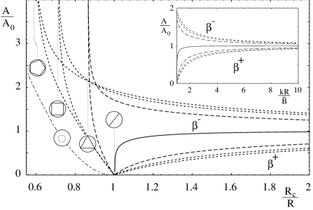
Figure 18: The amplitudes of the dominating orbits $\beta=(v,1)^{\pm}$ with $v=2,\dots,5$ relative to their $B=0$ value. (The amplitude of the cyclotron orbit is in arbitrary units.) At the bifurcation points $R_{c}=\sin(\pi\;v/w)$ indicated by vertical lines, the amplitudes diverge. For $R_{c}>R$ the amplitudes of the bouncing orbits quickly approach their asymptotic (zero-field) value. The inset shows this convergence in a wider range of $\widetilde{B}$.

The amplitudes of the “–” orbit is always larger than that of the corresponding “+” orbit. At $R_{c}=R$,where the “+” orbits change the topology (see Fig. 3), their amplitudes are zero, so that these bifurcations do not lead to artifacts in the level density. In stronger fields, the amplitudes diverge at the bifurcation points, indicating that the semiclassical approximation breaks down at these points (more exactly, one of the saddle-point approximations in the derivation of the trace formula becomes invalid). A rigorous treatment of these bifurcations has been presented in a very general form for two-dimensional systems by Ozorio de Almeida and Hannay [28], more explicit calculations have been performed, for example, by Kus et al. [29] and Sieber [30]. The main idea is always to replace the saddle-point approximation by a better adapted uniform integration. An application to the disk billiard has not been attempted here and will be the subject of further studies.

For the interpretation of the shell structure, let us first look at the weak-field regime ($R_{c}>R$). The amplitudes for zero field given in Eq. (26) are proportional to $v^{-1/2}$, favoring orbits with a small number of bounces $v$. The dependence of the amplitudes on the magnetic field as shown in Fig. 18 indicates that in the region where the “–” orbits differ significantly from the “+” orbits, the latter are negligible. These effects together strongly favor the $(2,1)$ and the $(3,1)^{-}$ orbits. They end up with comparable amplitudes. From this picture we expect as the dominating feature of the level density a pronounced beating pattern from the interference of the diameter and the triangular orbit. This beating pattern is well known for the zero-field case. In three-dimensional metal clusters, it is usually referred to as supershell oscillations [31]. Our description suggests that this beating will survive in homogeneous magnetic fields up to a strength of $\widetilde{B}=kR$. This is indeed observed, as seen in Fig. 16. The thick lines in the frames (1a) and (1b) correspond to a function

$$\sin(kG_{(1,2)})+\sin(kG_{(1,3)^{-}})=$$

$$\hskip 56.9055pt\sin\left(k\frac{\Delta G}{2}\right)\;\sin\left(k\frac{\bar{G}}{2}\right)\quad.$$ (27)

It predicts correctly the structure of the level density in this regime.

Approaching the field strength where $R_{c}=R$, all orbits change $G$ sharply to $2\pi$, so that they interfere coherently, forming the whispering gallery mode. We therefore expect that the beating behavior will disappear, leaving just a simple oscillation with the common frequency. In Fig. 16 this sudden stop of the beat at $R_{c}=R$ can be clearly seen. The solid line in frame 2 shows that the frequency of the remaining single oscillation is predicted correctly.

For $R_{c}<R$, the influence of the cyclotron orbits increases with stronger fields. The large amplitudes of the bouncing orbits near the bifurcation points is, as we have already pointed out, unphysical and should be removed by a rigorous treatment of the orbit bifurcations. For strong fields, only cyclotron orbits and bouncing orbits with a great number of bounces $v$ exist. The amplitudes of the latter are proportional to $v^{-1/2}$, so that in very strong fields we expect that the cyclotron orbits dominate the level density. The gray lines in frame 3 of Fig. 16 show the corresponding oscillating term, which, indeed, reproduces the main feature of the quantum-mechanical result (solid black). The skipping orbits with greatest amplitudes are those close to their bifurcation points. As can be seen in Fig. 17, all those orbits have nearly the same value of $G=w\cdot\pi^{2}R$. Their contributions should therefore interfere constructively, giving rise to small structures in the level density of this period. Such structures can indeed be observed in a higher-resolution spectrum, as shown in Fig. 15. The spacing of the small peaks between the Landau levels is, indeed, consistent with our simple picture.

Altogether we could show that this simple semiclassical picture is able to explain the main features of the quite complicated behavior of the level density for arbitrarily strong fields in terms of just 3 classical periodic orbits. We have here interpreted the dependence of the level density on the energy, but a completely analogous approach for the dependence on the magnetic field is possible.

6 Summary

We have derived a trace formula for the oscillating part of the level density of a circular billiard in homogeneous magnetic fields. We have used the general approach of Creagh and Littlejohn and compared our findings with the quantum-mechanical solution. In the weak-field domain, where the classical cyclotron radius $R_{c}$ is larger than the disk radius $R$, the agreement is excellent and even a full quantization, e.g., the resolution of the level density into individual energy levels, is possible.
In stronger fields, the quality of the standard semiclassical approximation is not satisfactory, even for the gross-shell structure. We have identified boundary effects to be responsible for the major part of the deviations. To implement these effects in the semiclassical trace formula, we have replaced the (discrete) Maslov index by a (continuous) reflection phase. The latter was calculated in a simple one-dimensional approximation. With this correction, the semiclassical approximation to the exact quantum-mechanical level density is good for all field strengths and energies. For a correction of the remaining deviations it would be necessary to include diffractive orbits and the effects of the orbit bifurcations. The orbit bifurcations at strong field strengths affect the shell structure only to a small extent, their influence on the full quantization is even smaller. The diffractive orbits do not influence the shell structure but only the full quantization. Both effects can therefore be neglected for the semiclassical description of the gross-shell structure. The reflection phases, however, are a crucial correction for both the gross-shell structure and the full quantization.

One advantage of the semiclassical description is its easy numerical evaluation. Much more attractive, however, is the simple, intuitive picture gained from it. Quantum mechanics readily gives information on individual levels or level statistics, which are hard to derive semiclassically. But the experimentally important long-range correlations of levels, leading to shells and supershells, are very easy to explain semiclassically. For a qualitative description of the shell structure just one or two classical periodic orbits are sufficient. In strong fields the single oscillation of the cyclotron orbits dominates and the coherent superposition of the strongest skipping orbits gives rise to additional small structures with much smaller spacing. For field strengths with $R_{c}\mbox{\raisebox{2.15277pt}[-2.15277pt][0.0pt]{$\scriptstyle<$} \raisebox{-8.61108pt}[0.0pt][-8.61108pt]{\Large\char 126\relax}}R$ the skipping orbits form coherently the whispering gallery mode, which gives rise to a single oscillation of the level density. In weak fields, the interference between the diameter and the triangular orbit dominates the level density. A quantitative semiclassical description is already possible including between 10 and 20 orbits. Future studies will be aimed at a rigorous treatment of the orbit bifurcations and an implementation of diffractive effects.

Acknowledgments
It is a great pleasure to thank Stephen Creagh for his continued interest in this work. He inspired many of the ideas presented here, helped to shape them in discussions, and gave valuable comments on the manuscript. We also thank Stephanie Reimann for stimulating discussions. This work has been supported by the Commission of the European Communities under Grant No. CHRX-CT94-0612.

Appendix A Geometrical quantities of the PO

The geometrical lengths $c$, $d$, and $s$ and the angles $\Theta$, $\gamma$, and $\varphi$ sketched in Fig.6 can be expressed in terms of the classical cyclotron radius $R_{c}$, the disk radius $R$ and the classification parameter $\beta^{\pm}=(v,w)^{\pm}$ as follows:

$$\Theta = \frac{w}{v}\pi\quad,$$

$$\gamma = \arcsin\left(\frac{R}{R_{c}}\sin\Theta\right)\quad,$$

$$\varphi = \left\{\begin{array}[]{rcccll}\gamma&-&\Theta&+&\pi/2&\mbox{for }(\beta^{+},R_{c}>R)\\ -\gamma&+&\Theta&+&\pi/2&\mbox{for }(\beta^{+},R_{c}<R)\\ \gamma&+&\Theta&-&\pi/2&\mbox{for }(\beta^{-})\quad,\end{array}\right.$$ (31)

$$c = R\cos\varphi\quad,$$

$$s = \sqrt{{R_{c}}^{2}-R^{2}\sin^{2}\Theta}\quad,$$

$$d = \left\{\begin{array}[]{ll}|s-R\cos\Theta|&\mbox{for }\beta^{+}\\ \,s+R\cos\Theta&\mbox{for }\beta^{-}\quad.\end{array}\right.$$ (34)

Appendix B Evaluating the PO sum

Semiclassical trace formulas are asymptotic series with non trivial convergence properties, so that they cannot be summed up straightforwardly. Frequently the Gaussian smoothing technique is used, which approximates the level density folded with a Gaussian by the trace formula where the amplitudes are damped by an additional (Gaussian) factor. This approach is limited to Gaussian line shapes and to smoothing of the level density in $k$. In this Appendix we introduce a more general approach, which can deal with arbitrary line shapes and smoothing variables. We will also state explicitly the conditions for the approximation to be valid.

The general form of a trace formula is given by

$$\delta g\;=\;\sum_{\Gamma}A_{\Gamma}(E)e^{i\frac{S_{\Gamma}(E)}{\hbar}-i\sigma_{\Gamma}\frac{\pi}{2}}\quad,$$ (35)

where $\Gamma$ is a one-dimensional classification of the classical periodic orbits. If there is a generalized energy $e(E)$, and functions $G(\Gamma,E)$ and $\tilde{\sigma}(G)$, which fulfill

$$\frac{S_{\Gamma}(E)}{\hbar}-\sigma_{\Gamma}\frac{\pi}{2}=eG-\tilde{\sigma}(G)\quad,$$ (36)

we can rewrite the trace formula as

$$\delta g\;=\;\sum_{G}A_{2}(e,G)e^{ieG}\quad.$$ (37)

Rescaling $G$ we can always obtain $G\in{\rm I\kern-1.79993ptN}$; the rescaling factors should be included in $A_{2}(e,G)$. Let us first assume that $A_{2}$ factorizes in terms that only depend on the generalized energy $e$ and the classification variable $G$:

$$A_{2}(e,G)=A_{G}(G)\;A_{e}(e)\quad.$$ (38)

Approximating Eq. (37) by an integral

$$\delta g\;\approx\;A_{e}(e)\int_{G}A_{G}(G)e^{ieG}\mbox{d}G\quad.$$ (39)

gives (apart from normalization constants) the oscillating part of the level density $\delta g$ as the Fourier transform of $A_{G}(G)$:

$$\delta g(e)\approx\sqrt{2\pi}\;A_{e}(e)\;{\cal F}[A_{G}(G)]\quad.$$ (40)

For an arbitrary window function $F(G)$ we get, using the well-known folding theorem,

$$\int_{G}F(G)A_{2}(e,G)e^{ieG}\mbox{d}G\approx\delta g(e)\ast f(e)\quad.$$ (41)

Here $f(e)$ denotes the Fourier transform of $F(G)$ and “$\ast$” stands for the convolution integral. Therefore we have

$$\delta g^{F}:=\sum_{\Gamma}F(G)A_{\Gamma}(E)\;e^{i\frac{S_{\Gamma}(E)}{\hbar}-i\sigma_{\Gamma}\frac{\pi}{2}}\approx\delta g(e)\ast f(e)\;,$$ (42)

where $\delta g^{F}$ denotes the trace formula with damped amplitudes. This relation shows that folding the semiclassical level density with a smoothing function $f(e)$ is equivalent to a multiplication of the amplitudes with a window function $F(G)$. Unfortunately the restrictions of Eqs. (36) and (38) are quite severe and often prevent the application of Eq. (42). With two additional approximations we can relax these restrictions. In the general case Eq. (38) is violated and we may just separate out a common dependence of the amplitudes on $e$:

$$A_{2}(e,G)=A_{G}(e,G)\;A_{e}(e)\quad.$$ (43)

In this case Eq. (42) is still a good approximation if $A_{G}(e,G)$ is sufficiently slowly varying in $e$. If we denote the characteristic width of $f(e)$ with $\gamma$, this means that $A_{G}(e,G)$ has to be nearly constant over a region $\gamma$ in $e$. If, on the other hand, there are no functions $e(E)$ and $G(E,\Gamma)$ that fulfill Eq. (36), a local expansion of the action $S$ in powers of $e$ can be used:

$$\frac{S}{\hbar}=\frac{S(e_{0})}{\hbar}+G(e_{0})\;(e-e_{0})+{\cal O}(e-e_{0})^{2}\quad.$$ (44)

If this approximation is good in a region in $e$ wider than the typical width $\gamma$ of the smoothing function, Eq. (42) still holds. In the general case $G$ is therefore given by the first derivative of the classical action with respect to $e$:

$$G(E)=\left.\frac{1}{\hbar}\frac{\mbox{d}S}{\mbox{d}e}\right|_{E}\quad.$$ (45)

With $e=E$, $\hbar G$ is the period $T$ of the orbit, so that we refer to $\hbar G$ as the quasiperiod. For systems with constant absolute velocity along the orbit (this holds especially for billiards), we get for the choice $e=k$

$$\frac{\mbox{d}S}{\mbox{d}e}=\frac{\mbox{d}S}{\mbox{d}E}\frac{\mbox{d}E}{\mbox{d}k}=T\cdot\frac{k\hbar^{2}}{m}=\hbar L\quad,$$

where $L$ is the geometrical orbit length. Putting all approximations together, we have shown that damping the amplitudes in the trace formula with a window function depending on $G$ gives an approximation for the level density folded with the Fourier transform of the window function used:

$$\delta g^{F}\approx f(e)\ast\delta g\quad.$$ (46)

This is the main result of this Appendix. The approximation holds if in a region wider than the typical width $\gamma$ of the smoothing function the conditions

$$S\approx S(e_{0})+G(e_{0})\;(e-e_{0})$$ (47)

and

$$A_{2}(e,G)\approx{\rm const}$$ (48)

are fulfilled. These conditions depend mainly on the behavior of the actions and amplitudes. In order to match them, a well-adapted choice of the generalized energy is essential. Note that for narrow smoothing functions (small $\gamma$), the conditions are less restrictive. Therefore for a full quantization the use of Eq. (46) is often justified, whereas for the calculation of the gross-shell structure the conditions Eqs. (47) and (48) put tight limits on the use of the amplitude damping ansatz – which might seem counter-intuitive at first sight.

We now illustrate the result with a simple example. Pure billiard systems are those where the the action along the orbits scales with the wave number: $S=\hbar k\cdot L$, and $L$, the geometric orbit length, is independent of the energy. Setting

$$e(E)=k=\sqrt{\frac{2mE}{\hbar^{2}}}\quad{\rm and}\quad G(\Gamma)=L\quad,$$ (49)

Eq. (47) is fulfilled trivially. If Eq. (48) is also matched, then the use of a window function $F$ depending on the orbit length $L$ is equivalent to a folding of the level density in $k$. Using a Gaussian window function we get a Gaussian smoothing of the level density in $k$ space. This is the technique frequently applied when evaluating trace formulas for billiard systems. Equation (46) is somewhat more general, as it is not restricted to billiard systems nor to special window functions. It makes (at least in principle) the calculation of arbitrary line shapes within the POT possible. It can also be used for an estimation of the effects of a (numerical) truncation of the trace formula, which can be thought of as a special window function. More important, however, are Eqs. (47) and (48), which give the limits of validity of the amplitude damping formula (46).

B.1 Evaluation for the circular billiard

We want to apply the considerations of the last section on the circular billiard. The natural choice for the generalized energy is $k$. Then the quasiperiod is the geometrical orbit length, given by

$$G=vr\cdot\left\{{\begin{array}[]{cccp{3mm}l}2\pi&-&2\gamma&&\mbox{for}\;(\beta^{+},R_{c}<R)\\ &&2\gamma&&\mbox{otherwise.}\end{array}}\right.\quad$$ (50)

Note that for $R_{c}>R$ (weak fields) $G$ is independent of the direction of motion $\pm$.
For computing the trace formula we have to choose an appropriate window function. As we want to compare the semiclassical result with the exact quantum-mechanical one, we look for a window function that can be Fourier transformed analytically. The usual Gaussian is nonzero for all $G$ and has to be truncated, being thus no longer analytically Fourier transformable. We used a triangular window instead, which matches all our demands. In order to make our results comparable with the usual Gaussian smoothing, we characterize the window function with a parameter $\tilde{\gamma}$, which corresponds to the variance of a Gaussian $\exp[-1/2(k/\tilde{\gamma})^{2}]$ with the same half-width.

We still have to check if the conditions (47) and (48) hold. They depend on the behavior of the amplitudes that are plotted in Fig. 18. At the bifurcation points the orbit amplitudes diverge, so that Eq. (48) is violated. For the evaluation in the corresponding regions we have therefore used a numerical folding procedure and evaluated directly the right-hand-side of Eq. (46).
For the cyclotron orbits discussed in Sec. 4.3 we get $G=n\cdot 2\pi R_{c}$ and $A=(2E_{0})^{-1}(1-R_{c}/R)^{2}$, which is slowly varying in the whole energy range. For the cyclotron orbits, approximation (46) is therefore justified for all $\widetilde{E}$ and $\widetilde{B}$.

References

- [1] Harris, J. J., Pals, J. A., and Woltier, R., Rep. Prog. Phys. 52, 1217 (1989).
- [2] Weiss, D., Richter, K., Menschig, A., Bergmann, R., Schweizer, H., von Klitzing, K., and Weimann, G., Phys. Rev. Lett. 70, 4118 (1993).
- [3] Darnhofer, D., Suhrke, M., and Rößler, U., Europhys. Lett., 35, 591 (1996).
-
[4]
Genzken, O., and Brack, M., Phys. Rev. Lett. 67, 3286 (1991);
Brack, M., Rev. Mod. Phys. 65, 677 (1993). -
[5]
Persson, M., Lindelof, P.E., von Sydow, B.,
Pettersson, J. Kristensen, A.
J. Phys. Condens. Matter 7, 3773 (1995);
Persson, M., von Sydow, B.,Lindelof, P.E., Kristensen, A., and Berggreen, K.-F. Phys. Rev. B 12, 8921 (1995). - [6] Berggreen, K.-F., Ji, Z.-L., and Lundsberg, T., Phys. Rev. B 54, 11612 (1996).
- [7] Reimann, S. M., Persson, M., Lindelof, P. E., and Brack, M., Z. Phys. B 101, 377 (1996).
- [8] Ullmo, D. , Richter, K., and Jalabert, R. A., Phys. Rev. Lett. 74, 383 (1995).
- [9] Tanaka, K., (unpublished).
- [10] Geerinckx, F., Peeters, M., and Devreese, J. T., J. Appl. Phys. 68, 3435 (1990).
- [11] Klama, S., and Rößler, U., Ann. Phys. (Leipzig) 1, 460 (1992).
-
[12]
Wentzel, G., Z. Phys. 38, 518 (1926);
Kramers, H. A., ibid. 39, 828 (1926);
Brillouin, M. L., Phys. Radium 6, 353 (1926). -
[13]
Keller, J. B., Ann. Phys. (Leipzig) 4, 180 (1958);
Keller, J. B., Rubinov, S. I., ibid. 9, 24 (1960). - [14] Berry, M. V., and Tabor, M., Proc. R. Soc. London, Ser. A. 349, 101 (1976); 356, 375 (1977).
- [15] Balian, R, and Bloch, C., Ann. Phys. (N.Y) 69, 76 (1972); 85, 514 (1974).
- [16] Gutzwiller, M. C., J. Math. Phys. (N.Y.) 11, 1791 (1970); 12, 343 (1971).
-
[17]
Strutinsky, V. M., Nukleonik 20, 679 (1975);
Strutinsky, V. M., and Magner, A. G., Elem. Part. & Nucl. (Atomizdat, Moscow) 7, 365 (1976) [Sov. J. Part. Nucl. 7, 138 (1976)]. -
[18]
Creagh, S. C., and Littlejohn, R. G.,
Phys. Rev. A 44, 836 (1990);
J. Phys. A 25, 1643 (1991).
- [19] Brack, M., and Bhaduri, R. K. Semiclassical Physics (Addison and Wesley, Reading, 1997).
-
[20]
Tatievski, B., Stampfli, P., and Bennemann, K. H.,
Comput. Mater. Sci. 2, 459 (1994);
Tatievski, B., Diplomarbeit, Freie Universität Berlin, (1993) (unpublished). - [21] Bogachek, E. N., and Gogadze, G. A., Zh. Eksp. Teor. Fiz. 63, 1839 (1973) [Sov. Phys. JETP 36, 973 (1973)].
- [22] Reimann, S. M., Brack, M., Magner, A. G., Blaschke, J., and Murthy, M. V. N., Phys. Rev. A 53, 39 (1996).
- [23] Brack, M., and Jain, S. R., Phys. Rev. A 51, 3462 (1995).
- [24] Creagh, S.C. J. Phys. A 26, 95 (1993); Ann. Phys. 248, 60 (1996).
- [25] Reimann, S. M., Brack, M., Magner, A. G., and Murthy, M. V. N., Surf. Rev. Lett. 3, 19 (1996).
- [26] see, e.g., Baltes, H. P., and Hilf, E. R.: Spectra of Finite Systems (Bibliographisches Institut, Mannheim, 1972)
- [27] Isihara, A., and Ebina, K., J. Phys. C 21, L1079 (1988)
- [28] Ozorio de Almeida, A. M., and Hannay, J. H., J. Phys. A 20, 5873 (1987).
- [29] Kus, M., Haake, F., and Delande, D., Phys. Rev. Lett. 71, 2167 (1993).
- [30] Sieber, M., J. Phys. A 29, 4715 (1996).
- [31] Nishioka, H., Hansen, K., and Mottelson, B. R., Phys. Rev. B 42, 9377 (1990).