[

A Creation Operator for Spinons in One Dimension

Abstract

We propose a definition for a creation operator for the spinon, the fractional statistics elementary excitation of the Haldane-Shastry model, and give numerical and analytical evidence that our operator creates a single spinon with nearly unit amplitude in the ISE model. We then discuss how the operator is useful in more general contexts such as studying the underlying spinons of other spin chain models, like the XXX- and XY-model, and of the one dimensional Hubbard model.

]

One of the deepest open problems in condensed matter physics today is that of understanding fractional statistics, that is understanding field theories whose underlying excitations do not obey either Bose or Fermi statistics. Such possibilities (fractional statistics) for point particles are forbidden in three dimensions; however, in two dimensions, braid statistics can occur and anyons [1] are allowed, while, in one dimension, there exist parafermion operators [2] which also do not obey Fermi or Bose statistics. Such fractional statistics objects may be important for describing the low energy excitations of condensed matter systems if these systems are categorized by fixed points whose effective, low energy Hamiltonians are one or two dimensional.

The Heisenberg model with inverse squared exchange (ISE) [3, 4] ($H=\sum_{i,j}(\frac{N}{\pi}\sin\pi\frac{i-j}{N})^{-2}{\bf S}_{i}\cdot{\bf S}_{j}$) is believed to provide a model whose excitations are completely non-interacting fractional statistics particles [5, 6] referred to as spinons. The statistics of these excitations are most naturally discussed in terms of an alternative definition, proposed by Haldane [7], in which a particle’s statistics is defined in terms of its effect on the size of Hilbert space for other particles. For example, on the lattice, each fermion added to a system decreases the number of states in the Hilbert space for other fermions of the same type by one, while each added boson leaves the size of the available Hilbert space unchanged. Fractional exclusion statistics occurs for operators which reduce the Hilbert space by a non-integer amount, i.e. at a fraction of the rate for fermions. This definition has been shown to agree with the definition of statistics through particle interchange in the case of the quasiparticles of the Laughlin state (when the cut-offs in the theory are treated carefully) [7, 8, 9]. In that case, the change in the phase of the wavefunction resulting from quasihole interchange is the same fraction of $\pi$ as the rate of Hilbert space reduction due to the creation of quasiholes, relative to the rate of reduction due to the creation of fermions.

For the exclusion approach, lattice models are more natural since the number of states in the Hilbert space is easily defined, and, indeed, Haldane introduced his definition partially motivated by results for the ISE spin chain model: the spectrum of the ISE spin chain model can be described with a set of non-interacting single particle energies, and a set of rules for the occupation of the single particle levels which embody the Yangian symmetry of the model [5]. The effect of these rules is that the creation of spinons eliminates allowed spinon states (of any polarization) from the Hilbert space half as fast as the creation of fermions eliminates allowed fermion single particle states from a Hilbert space of fermionic states [10]. The spinons are thus half-fermions or semions and are completely free. This property makes the ISE model somewhat more natural for studying exclusion statistics than the Laughlin states since the quasiholes are not ideal fractional exclusion statistics particles [11].

In light of this, it would be very useful to have some method of treating the underlying spinons in that and related models beyond the first quantized formalism; one would like to introduce spinon creation and annihilation operators. The main purpose of this work is to introduce an operator which has essentially unit overlap with the spinon creation operator in the ISE model, and which, we conjecture, can be interpreted as a spinon creation operator much more broadly than this.

The operator we now propose was motivated chiefly by the behavior of the large $U$ wavefunction of the Hubbard model [12], which factorizes into spin and charge parts which are linked only by a backflow condition [12]. Except for the backflow condition, the charge part is described by free spinless fermion wavefunction and the spin part by a wavefunction of the one dimensional Heisenberg model ($H=\sum_{i}{\bf S}_{i}\cdot{\bf S}_{i+1}$) where the role of the sites is played by the electrons. The creation operator for an up spin electron in that model involves the creation of a spinless fermion in the charge wavefunction, the backflow and the insertion of a site with an up spin into the Heisenberg model wavefunction. Likewise, the bosonization approach to the Hubbard model [13] exhibits a similar spin charge decoupling, with the electron creation operator effectively factorizing into a product of exponentials in spin and charge density eigenexcitations. This suggests the identification of the spin insertion with the spin boson part of the electron operator. Further, the spin operator is identical to the primary field of the $c=1$ conformal field theory studied in [14], and the Fourier models of this operator are also recognizable as a semionic parafermion. Thus, it has the essential properties expected of a spinon operator, being both semionic and providing a natural representation of the Yangian [14].

We therefore conjecture that the local up-spinon creation operator might be given approximately by an operator, $O^{\dagger}(x)$, which inserts an additional up-spin into a one-dimensional spin chain after site $x$ but before site $x+1$. Peculiarly, this operator, in the process of creating a spinon, would have to change the length of the spin chain it acted on from $N$ to $N+1$. Some such an exotic effect is clearly necessary in defining a single spinon creation operator because of the fractional exclusion statistics of the spinon; an operator which creates a single spinon must involve the rearrangement of the Hilbert space different from what occurs for fermions or bosons and hence the need to change the number of sites in the model in order to create a single spinon. We have discussed this feature of exclusion statistics before in a slightly different context involving spin chains [15], and it also occurs in the case of Laughlin wavefunctions restricted, for example, to the sphere where the creation operator involves an addition of allowed states to the (appropriately cut-off) Hilbert space.

If we accept this unusual property as an unavoidable complication for fractional statistics operators, the evidence is there to support the proposal that the spin insertion creates a single spinon with the same polarization. Let us first study this conjecture in the context of the ISE model. In complete analogy with the insertion of two spins in a singlet [15], we can construct the state obtained by inserting a single spin. To fix notation: the unnormalized groundstate wavefunction on $N$ (even) sites of the ISE model in a basis labeled by the positions of the down-spins $\left\{n_{1},\ldots,n_{M}\right\},\,M=\frac{N}{2}$ is given by:

$$\Psi^{(0)}_{N}\left(n_{1},\ldots,n_{\frac{N}{2}}\right)=\prod_{i=1}^{\frac{N}{2}}(-)^{n_{i}}\prod_{i<j}^{\frac{N}{2}}\sin^{2}\left(\frac{n_{i}-n_{j}}{N}\pi\right).$$ (1)

In a basis of local spins $\{|\sigma_{1}\cdots\sigma_{N}\rangle\}$, $\sigma_{i}=\pm\frac{1}{2}$ this reduces to [16]:

$$\Psi^{(0)}_{N}\{\sigma_{1}\cdots\sigma_{N}\}=\prod_{i<j}^{N}(z_{i}-z_{j})^{\delta_{\sigma_{i},\sigma_{j}}}e^{\frac{\pi i}{2}\rm{sgn}(\sigma_{i}-\sigma_{j})}.$$ (2)

For the even $N$-site ISE groundstate $\{z_{i}\}\equiv C_{N}=\{e^{\frac{2\pi in}{N}};n=1\ldots N\}$. The action of $O^{\dagger}(x=N)$ on this state is, in the language of eq. (2), to add an extra spin $\sigma_{N+1}=\uparrow$, and leave the other spins alone (with trivial generalization to other values of the insertion-site $x$).

In order to answer the question, to what extent this state $O^{\dagger}(x)|\Psi^{(0)}_{N}\rangle$ simulates a true 1-spinon state, let us recall what the latter looks like [16, 17]. Since the ISE-Hamiltonian commutes with momentum, the 1-spinon eigenstates (which exist only for an odd number of sites) have definite momentum. However these states can be coherently superimposed (Fourier transformed) into states in which the single spinon is completely localized on a site, say $x$, which is no longer an eigenstate of $H_{\rm ISE}$. Such an unnormalized state is known to be [16, 17] of the form

$$\Psi^{(1)}_{N+1}(n_{1}\ldots n_{\frac{N}{2}}|x)=$$ (4)

$$\prod_{i=1}^{\frac{N}{2}}(-)^{n_{i}}\sin(\frac{n_{i}-x}{N+1}\pi)\prod_{i<j}^{\frac{N}{2}}\sin^{2}(\frac{n_{i}-n_{j}}{N+1}\pi),$$

in the language of down-spin co-ordinates $\{n_{i}\}$. In terms of spin co-ordinates $\{\sigma_{1}\ldots\sigma_{N+1}\}$ it looks exactly like eq. (2)[18]:

$$\Psi^{(1)}_{N+1}=\prod_{i<j;\,i,j\neq x}^{N+1}(z_{i}-z_{j})^{\delta_{\sigma_{i}\sigma_{j}}}e^{\frac{\pi i}{2}{\rm sgn}(\sigma_{i}-\sigma_{j})},$$ (5)

but $\sigma_{x}$ is excluded from the product (since $\sigma_{x}$ is fixed to be up), and the set $\{z_{i}\}\equiv C_{N+1}=\{e^{\frac{2\pi i}{N+1}};\,n=1\ldots N+1\}/\{z^{\frac{2\pi ix}{N+1}}\}$. Notice that in the $\{\sigma_{i}\}$-basis the quasihole-factor in (4) goes away. Our conjecture is now that $|\Psi^{(1)}_{N+1}(x)\rangle\simeq O^{\dagger}(x)|\Psi^{(0)}_{N}\rangle$. Numerically it turns out that the two states have an excellent overlap: $\frac{\langle\Psi^{(1)}_{N+1}(x)|O^{\dagger}(x)|\Psi^{(0)}_{N}\rangle}{\parallel\Psi^{(1)}_{N+1}(x)\parallel\cdot\parallel\Psi^{(0)}_{N}\parallel}=0.984+{\cal O}(N^{-\frac{3}{2}})$. This is unsurprising, since $|\Psi^{(1)}_{N+1}(x)\rangle$ is obtained from $O^{\dagger}(x)|\Psi^{(0)}_{N}\rangle$ by adiabatically deforming the set of $N$ $z_{r}$’s: $e^{\frac{2\pi i}{N}\cdot r}\rightarrow e^{\frac{2\pi i}{N+1}\cdot r}$, and leaving the single spin(on) at site $x$ alone, see Fig. 1. Although this is an uncontrolled approximation, it seems justified by the high numerical overlap.

Naively one might expect from eq. (4) there to be $(N+1)$ 1-spinon states; there is, however, a reduction, because only $\frac{N+2}{2}$ of these are linearly independent. This can be seen by reconstructing the momentum eigenstates, through Fourier transforming eq. (4) in the spinon co-ordinate $x$. This transform only has support in the range $[-\frac{\pi}{2},\frac{\pi}{2}]$ ($N=4m$) or $[\frac{\pi}{2},\frac{3\pi}{2}]$ ($N=4m+2$). One notices that the states thus obtained are indeed eigenstates, since (1) the set $\{\Psi^{(1)}_{N+1}(x)|x=0\ldots N\}$ spans the 1-spinon subspace [16], and (2) there is only one up-spinon eigenstate for a fixed value of momentum.

As stated before, spinons in eigenstates are not localized but have a momentum so that we must investigate to what extent our spin insertion can be connected with spinon creation in momentum space. Since the number of sites in the chains before and after the action of the spinon operator is different, the definition of the spinon creation operator of fixed momentum is not trivial and the Fourier transform of the creation operator requires some care. If we define the momentum space version of the creation operator by:

$$O^{\dagger}(k_{N+1}-q_{N})=\frac{1}{\sqrt{N+1}}\sum_{x=0}^{N}e^{i(k_{N+1}-q_{N})x}O^{\dagger}(x)$$ (6)

where $k$ is an allowed momentum in the $N+1$ site model and $q$ is an allowed momentum in the $N$ site state, then, the operator takes a momentum eigenstate of the $N$ site model to an momentum eigenstate of the $N+1$ site model. (In the following we will assume periodic boundary conditions, but other boundary conditions can be implemented straightforwardly). In particular, if $N$ is a multiple of 4 then the groundstate has zero momentum and $q$ can be taken to be zero if we wish to create a single excited spinon. In this case, this construction allows us to study our approximation to the single spinon spectral function defined by:

$$A_{s}(k,\omega)=\sum_{m}|\langle m|O^{\dagger}(k_{N+1})|GS\rangle|^{2}\delta(E_{m}-E_{0}-\omega)$$ (7)

where the sum over $m$ is over a complete set of eigenstates of the $N+1$ site model and $|GS\rangle$ is the groundstate of the $N$ site model. If our conjecture were a perfect spinon creation operator, then for the ISE model the spectral function would be a $\delta$-function of unit weight located on the 1 spinon dispersion relation $\varepsilon_{s}(k)=\frac{1}{2}((\pi/2)^{2}-k^{2})$.

The actual result is remarkably close to this as shown in Figure 2. For the finite systems that we studied (up to 24 sites), for the ISE model, at least 99.4% of the weight of the spin insertion seems to lie on the single spinon. However the weight in the spectral function for $O^{\dagger}$ is not unity (as it would be for $c^{\dagger}_{k}$ in the case of free bosons or fermions), nor is it close to it, since we don’t know a priori how to normalize our spinon operator such that it creates a normalized state. However, for the ISE, using the aforementioned almost-equivalence of spin-inserted wavefunction and the localized spinon wavefunction, we can get an idea of what this normalization should be like. That is, we will find the normalization appropriate if the spin-insertion put all of its weight in the one-spinon state (rather than just 99%). Then we need only compute the contribution to the normalization from the matrix element in (7), for the 1 spinon state (of momentum $Q=k$). The weight $A(k,\varepsilon_{s}(k))$ is given by (in an obvious notation):

$$\sqrt{NC^{(0)}C^{(1)}}A(k) = \langle\Psi^{(1)}_{N+1}(Q=k)|\cdot\sum_{j=0}^{N}|\Psi^{(1)}_{N+1}(j)\rangle e^{-ikj}$$ (8)

$$= \sum_{i,j=0}^{N}\langle\Psi_{N+1}^{(1)}(i)|\Psi_{N+1}^{(1)}(j)\rangle e^{ik(i-j)},$$ (9)

where $C^{(0)}=\frac{N!}{M!}N^{M}2^{-M(N-1)}$ and $C^{(1)}=M!N^{M}2^{-M(N-1)}$ are the normalization of respectively states $\Psi_{N}^{(0)}$ (eq. 1) and $\Psi_{N+1}^{(1)}(x)$ (eq. 4). The relevant matrix element in the RHS of this equation, involving sums over locations of down-spins, can be computed, after one realizes that these sums can be replaced by integrals of the same expression, due to the polynomial nature of the summand [3],[17]. Methods to compute integrals of this kind have been developed in the context of the Calogero-Sutherland model [4] and random matrices, using for instance Jack-polynomials, and matrix-model correlators[19, 20]. We will follow instead Sutherland’s recipe [4],[22]. There we find, after a little bit of algebra that ($M\equiv\frac{N}{2}$):

$$g(i-j) \equiv \langle\Psi_{N+1}^{(1)}(i)|\Psi_{N+1}^{(1)}(j)\rangle=\langle\prod_{l=1}^{M}u(\theta_{l})\rangle={\rm det}F_{p,q}$$ (10)

$$u(\theta) = \frac{1}{2}(\cos\left(\frac{i-j}{N}\pi\right)-\cos(\theta))$$ (11)

$$F_{p,q} = \int_{-\pi}^{\pi}\frac{d\theta}{2\pi p}u(\theta)\left\{p\cos\theta p\cos\theta q+q\sin p\theta\sin q\theta\right\}$$ (12)

$$= \frac{1}{4}\left\{\cos\left(\pi{\scriptscriptstyle\frac{i-j}{N}}\right)\delta_{pq}-\frac{1}{2}\delta_{p,q+1}-\frac{1}{2}\delta_{p,q-1}\right\}({\scriptscriptstyle 1+\frac{p}{q}})$$ (14)

$${\rm and\,\,}p,q=\frac{1}{2}\ldots M-\frac{1}{2}$$

If we set $x=\cos\left(\frac{i-j}{N}\pi\right)$ the ensuing (tridiagonal!) determinant observes the recursion relation:

$$d_{n+1}(x)=(2n+1)d_{n}(x)-n^{2}d_{n-1}(x)$$ (15)

with initial conditions $d_{0}=1,\,d_{1}=x$. This is exactly the definition of the Legendre Polynomials: $d_{M}(x)=M!P_{M}(x)$ (with normalization $P_{M}(1)=1$). Then the Fourier transform in eq. (9) is given by [23]:

$$A(k) = (N+1)\left({\scriptstyle\begin{array}[]{c}2r\\ r\end{array}}\right)\left({\scriptstyle\begin{array}[]{c}2(M-r)\\ M-r\end{array}}\right)2^{-2M}$$ (20)

$$\,\,\stackrel{{\scriptstyle\frac{1}{N}\ll\frac{\pi}{2}-k\ll 1}}{{\simeq}}\,\, \frac{2}{\sqrt{\left(\frac{\pi}{2}\right)^{2}-k^{2}}},$$ (21)

and $k=\frac{\pi}{2}-\frac{2\pi}{N+1}(r+\frac{1}{4})$. In the derivation we have chosen $M$ even to prevent cumbersome notation. See the remark above about where the weight is located, depending on the parity of $M$. We notice that the weight diverges at what Haldane calls the spinon “pseudo-fermi surface”. The square root divergence is exactly that expected for spectral function of the spin part of the electron operator obtained in Abelian bosonization; the exponent should be $\frac{K_{\sigma}}{4}+\frac{1}{4K_{\sigma}}=\frac{1}{2}$, for $K_{\sigma}=1$, i.e. isotropic spin exchange[24].

Although almost all of the effect of the operator defined by eq. 6 is to create a single spinon in an ISE models, there is some amplitude in the spectral function off the single spinon energy, so that our operator can not be taken to be identically the spinon creation operator. The connection between the two is rather like that between the bare electron operator and the quasiparticle operator in Fermi liquid theory: in addition to the expected $\delta$-function there are very small “incoherent” contributions coming from the fact that our creation operator has finite weight to create more than one spinon.

In any case, the operator will be extremely useful if we can demonstrate that it has large finite overlap with the spinon creation operator in a broader context than acting on the ground state of the ISE model. For example, the Heisenberg model is in the same universality class as the ISE model and can be thought of as a model of nearly free spinons (they have a marginally irrelevant interaction), and so we have displayed the spectral function of the spinon operator acting on the groundstate of that model together with the ISE spectral function in Figure 2. For both models there is very little probability to excite states with momentum, inside the “pseudo-fermi surface”, weight is down there by as much as 3 orders of magnitude, and, we see that, for the Heisenberg model, the weight is predominantly distributed on a 1-parameter family of states, which carries at least 98 % of the weight. Notice that the single spinon feature in the spectral function exists only over half the Brillouin zone as expected from the Bethe Ansatz solution of the Heisenberg model and the solution of the ISE model[3]. This is also consistent with the fact that the two species of spinon (up and down spin) should obey mutual $\frac{1}{2}$ statistics [25] so that the creation a spinon of either type reduces the Hilbert space of the spinon of the other type by $\frac{1}{2}$. This is realized here since adding one site and one spinon to the model adds only $\frac{1}{2}$ of a state for other spinons, because only one-half of the Brillouin zone is accessible. The interchange of two spinon insertion operators acting at different points, conversely does not yield a phase of $\pm\pi/2$; rather the leftmost spinon is shifted one site. However, in the low energy limit, the spinon lives near momentum $\pm\pi/2$ and the position shift mimics semionic statistics.

Both the ISE and Heisenberg models are exactly soluble and therefore well understood, however, our definition can be extended to essentially any one dimensional spin chain model, including anisotropic spin chain model such as the $XY$ model ($H=\sum_{i}S^{x}_{i}S^{x}_{i+1}+S^{y}_{i}S^{y}_{i+1}$). This model can be mapped onto a hard-core boson problem and then onto free fermions via a Jordan-Wigner transformation, so it is readily soluble, however, the connection between that solution and other viewpoints is still unclear. In particular, it should be possible to understand the $XY$ model as model of interacting spinons. If our spinon creation operator can really be taken as such then we can study the underlying, interacting spinons of $XY$ model and elucidate this connection—a possibility that would not exist were we restricted to the first quantized understanding of the spinons available for the ISE model. For example, we have computed the spinon spectral function as before for this model with the results shown in Figure 3.

They can be compared to the theoretical explanation based on the identification of the chiral parafermion, $\exp(i\frac{1}{\sqrt{2}}\theta^{R~{}{\rm or}~{}L}_{\sigma}(x))$, with the spinon. In that case, the Luttinger liquid hypothesis [26] for the XXZ chains predicts that the asymptotic correlations of the spinon in the $XY$ model should take the form

$$A_{\rm spinon}(x,t) \sim \frac{e^{i\pi x/2}}{(x-vt)^{9/16}(x+vt)^{\frac{1}{16}}}$$ (22)

$$+ {\rm left~{}moving~{}piece}+{\rm non-universal}$$ (23)

The universal properties of the spectral function can be computed from this [24] and it follows that: (1) the spinon spectral function has no $delta$-functions but rather power law singularities at $\omega=\pm vk$, with $k$ measured from $\pm\pi/2$, of the form: $|\omega-vk|^{-15/16}$ and $|\omega+vk|^{-7/16}$ and (2) the integral of the spectral function over frequency: $A(k)$ (which would simply be the $1-n_{k}$ for fermions or bosons) diverges like $k^{-\frac{3}{8}}$ as $\pm\pi/2$ is approached from either side. The ratio of the prefactors of the divergences is $\frac{\sin(7\pi/16)}{\sin(\pi/16)}\sim 5.03$. This agrees with our numerical results for this ratio for systems of large size (about 2000 sites for $A(k)$ and 100 for $A_{\rm spinon}(k,\omega)$). The power law rather than $\delta$-function divergence in $A_{\rm spinon}$ is quite obvious when we compare Fig. 2 and 3: ie. $O^{\dagger}(Q)$ has significant weight on a large number of states beyond the lowest-energy single particle-hole state. One apparent exception to this statement is spin-insertion with $Q\sim\pm\frac{\pi}{2}$: in that case the larger part of the weight remains on a single particle-hole state, even as $N\rightarrow\infty$. However, the relative weight on this class of free Jordan-Wigner fermion states decays as $[|\frac{\pi}{2}-Q|N]^{-\eta}$ with $\eta\simeq 0.1$ and vanishes (slowly) when we take $N\rightarrow\infty$ before $|Q|\rightarrow\frac{\pi}{2}$. Thus our spinon construction is in accord with all of the expected properties for a spinon creation operator in the $XY$ model.

An analog of our spinon operator can also be constructed for “spin” chains not based on $SU(2)$, such as the $SU(3)$ generalization of the nearest neighbor Heisenberg model in which the “spin” at each site is in the fundamental representation of $SU(3)$ [27] (This is the model that would naturally be obtained from an $SU(3)$ generalization of the large $U$ Hubbard model at $\frac{1}{3}$ filling). The results for the spectral function are shown in Fig. 4.

For the ISE and Heisenberg models, we knew that we were dealing with free or weakly interacting spinons, however, the existence of such spinons in the $SU(3)$ model, while plausible has not been shown. The spinon spectral function of Fig. 4 demonstrates that that model is also one of nearly free spinons. Our spinon creation operator construction is thus very useful in this context, yielding a powerful, qualitative result quite simply. Moreover, the spectral function we have obtained reveals that the spinons of the $SU(3)$ model are not semions but rather obey mutual $\frac{1}{3}$ statistics; that is the creation of one of any of the three spinon species reduces the Hilbert space for any of the three spinon species by $\frac{1}{3}$ of a state. This follows from the fact that the “spinon” spectral function has support only over $\frac{2}{3}$ (in general $\frac{p-1}{p}$ for SU($p$) spin models) of the Brillouin zone. These results are in agreement with findings for the ISE $SU(N)$ models [28] and demonstrate the the nearest neighbor model is almost certainly in the same universality class.

Our results for the spinon spectral function in the Heisenberg model are directly related to the work on the electron spectral function of the one dimensional Hubbard model [29, 30]. As a result of the completeness of the momentum space spinon operators for states reached by the insertion of a single spin, and the fact that our spinon creation operator creates a momentum eigenstate, the function $C_{\sigma}(k,\omega)$ of [29] is, in fact, identical to our $A_{s}(k,\omega)$. Their finding that the weight in $C_{\sigma}(k,\omega)$ is concentrated in half the Brillouin zone at the lowest allowed energies is a consequence of the fact that $C_{\sigma}(k,\omega)$ contains the single spinon spectral function plus small corrections coming from three and higher spinon terms. As a result, it is dominated by the single spinon part of the spectral function. This occupies only half the Brillouin as a consequence of the Yangian symmetry and fractional statistics of the spinons [5]. For the $XY$ model, (also studied in [29]) the spinons are interacting and even the single spinon contribution to the spectral function has weight over the entire Brillouin zone and a power law divergence as the threshold energy is approached from above. This behavior for $C_{\sigma}(k,\omega)$, was, in fact, independently obtained in [29].

In summary, we have proposed a spinon creation operator for one dimensional spin models and their generalizations. We have shown that the states created by the proposed operator have excellent, although not perfect, overlap with the actual one spinon eigenstates of the ISE model. In addition, for finite size Heisenberg models, nearly all of the operator’s weight when acting on the groundstate goes into creating an the eigenstate with the lowest possible energy for a given momentum—consistent with what expects for the single spinon creation operator given that the Heisenberg model is a model of spinons with marginally irrelevant interactions. For the $XY$ model, the operator acting on the groundstate creates states with a broad distribution of energies, but the detailed properties of the distribution are those expected for a spinon creation operator (if the $XY$ model is regarded as a Luttinger liquid model of strongly interacting semionic spinons). For an $SU(3)$ generalization of the Heisenberg model, we find results consistent with a straightforward generalization of the SU(2) spinon creation operator acting as a spinon creation operator for a system of weakly interacting “spinons” obeying Haldane type $\frac{1}{3}$ mutual exclusion statistics. This result is consistent with expectations but, to our knowledge, has not been demonstrated by any other means.

Together, these results indicate that the operator proposed is a valid spinon creation operator, and should be quite useful in the study of one dimensional spin models and their generalizations.

One of us (S.P.S) acknowledges support from Department of Energy grant DOE DE-FG02-90ER40542.

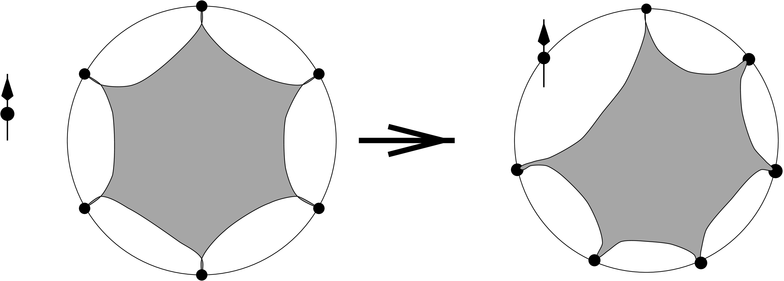
FIG. 1.: Graphical illustration of the deformation of the spin insertion to a spinon singlet insertion. The gray area is the groundstate wavefunction, or an adiabatic deformation thereof.

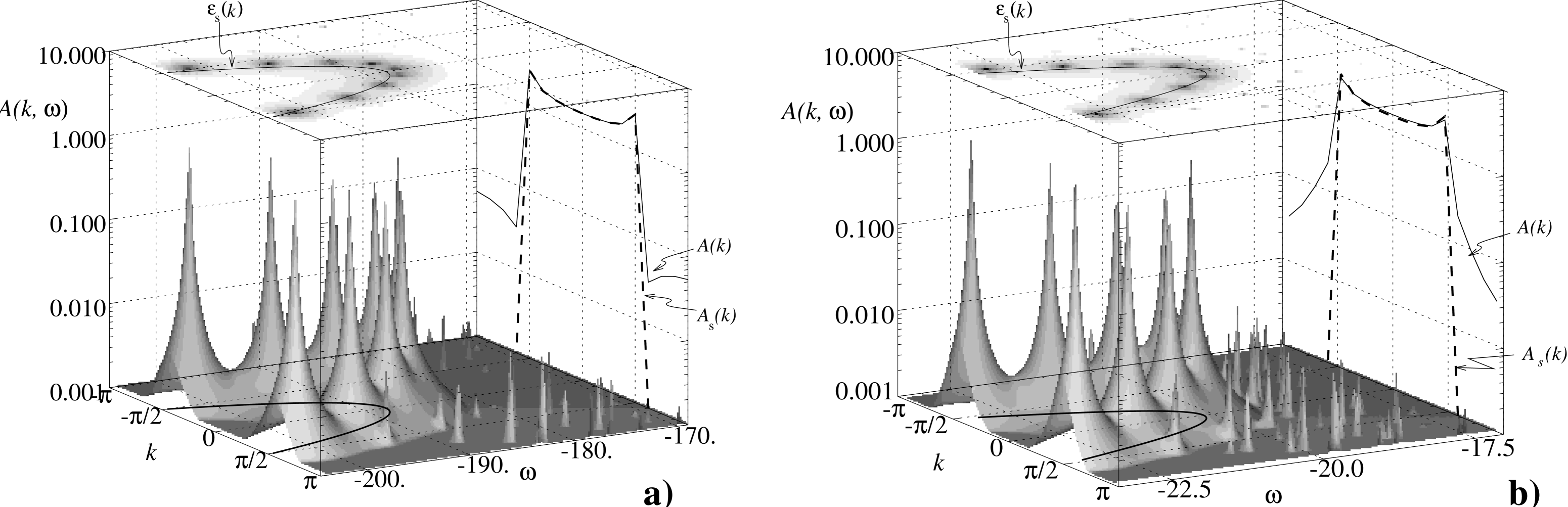
FIG. 2.: The spectral weight of the spin-insertion operator for (a) ISE and (b) Heisenberg 1D spin-chains, on 16 sites. The discrete data has been smoothed by convolving with a Lorentzian. Notice that the z-axis has a logarithmic-scale. Otherwise, on a linear scale, the multi-spinon contributions would not be visible! The solid line on the back wall, $A(k)$, is the $\omega$-integrated spectral weight, or equal time spin-insertion correlator. The dashed line is the contribution from single spinon states (the height of the large peaks). On the top we show a density-plot from which it is clear that virtually all the weight lies on the 1-spinon dispersion curve—$\varepsilon_{s}(k)=\frac{1}{2}((\frac{\pi}{2})^{2}-k^{2})$ for ISE and $\pi\cos(k)$ for the Heisenberg model [31].

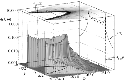
FIG. 3.: The spectral weight of the spin-insertion operator for the XY-model on 100 sites, allowing up to 3 particle hole excitations. The data has been smoothed by convolving with with a Lee-filter, and plotted on a log-linear scale. Notice that some finite weight seems to be present on the groundstates with momenta $-\frac{\pi}{2}\leq Q\leq\frac{\pi}{2}$; these contributions, however, vanish in the thermodynamic limit, except for the lowest energy states close to $\pm\frac{\pi}{2}$. The latter have measure 0, thus restoring results from bosonization. The curve on top is the 1 particle-hole dispersion, other symbols are as in fig. 2.

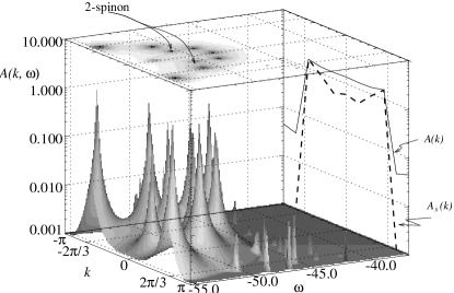
FIG. 4.: The spectral weight of the spin-insertion operator for the SU(3) Heisenberg model on 9 sites. The data has been smoothed by convolving with a Lorentzian and plotted on a log-linear scale. The symbols are as in fig. 2. Notice that in addition to the 1-spinon (’3’-representation) there is also some weight on states with 2 anti-spinons (’$\bar{3}$’-representation). This feature remains presumably as $N\rightarrow\infty$ [32].

REFERENCES

- [1] F. Wilczek, Phys. Rev. Lett. 48, 1144 (1982).
- [2] E. Fradkin and L. P. Kadanoff, Nucl. Phys. 170B, 1 (1980).
- [3] F.D.M. Haldane, Phys. Rev. Lett. 60, 635 (1988); B.S. Shastry, Phys. Rev. Lett. 60, 639 (1988).
- [4] B. Sutherland, Phys. Rev. A 4, 2019 (1971).
- [5] F. D. M. Haldane, Z. N. C. Ha, J. C. Talstra, D. Bernard and V. Pasquier, Phys. Rev. Lett. 69, 2021 (1992).
- [6] F.D.M. Haldane in Proc. of the 16th Tanaguchi Symposium on Condensed Matter, Kashikojima, Japan, Oct. 26-29, 1993,edited by A. Okiji and N. Kawakami (Springer-Verlag, Berlin-Heidelberg-New York, 1994).
- [7] F. D. M. Haldane, Phys. Rev. Lett. 67, 937 (1991).
- [8] R. B. Laughlin, Phys. Rev. Lett. 50, 1395 (1983); B. I. Halperin, Helv. Phys. Acta 56, 75 (1983); B. I. Halperin, Phys. Rev. Lett. 52, 1583 (1984); D. Arovas, J. R. Schrieffer and F. Wilczek, Phys. Rev. Lett. 53, 722 (1984).
- [9] Y.-S. Wu, Phys. Rev. Lett. 73, 922 (1994).
- [10] There are some complications related to that existence of two kinds of spinon as discussed later in the text.
- [11] C. Nayak and F. Wilczek, Phys. Rev. Lett. 73, 2740 (1994).
- [12] M. Ogata and H. Shiba, Phys. Rev. B41, 2326 (1990).
- [13] H. J. Schulz, Phys. Rev. Lett. 64, 2831 (1989); S. Sorella, A. Parolla, M. Parrinello and E. Tosatti, Europhys. Lett. 12, 729 (1990); H. Shiba and M. Ogata, Prog. Theor. Phys. Supplement 108, 265 (1992); M. Gulasci and K. S. Bedell, Phys. Rev. Lett. 72, 2765 (1994).
- [14] P. Bouwknegt, A. W. W. Ludwig, K. Schoutens, Phys. Lett. B 338, 448 (1994).
- [15] J.C. Talstra, S. P. Strong and P. W. Anderson, Phys. Rev. Lett. 74, 5256 (1995).
- [16] F.D.M. Haldane, Phys. Rev. Lett. 66, 1529 (1991).
- [17] J.C. Talstra and F.D.M. Haldane, Phys. Rev. B 50 6889 (1994).
- [18] The conversion from to basis is based on the identity when and lies on the lattice .
- [19] B.D. Simons, P.A. Lee, and B.L. Altshuler, Phys. Rev. B 48, 11450 (1993); Z.N.C. Ha, Phys. Rev. Lett. 73, 1574 (1994) and Nucl. Phys. B 435, 604 (1995); F. Lesage, V. Pasquier and D. Serban Nuc. Phys. B 435, 585 (1995).
- [20] Following the method of [21], now considering correlators of Pfaffians instead of determinants—just one spinon is created instead of two—we obtain a result, similar to the one in that reference, but now the final integral is not over a manifold of matrices , but matrices instead. At the saddle point this reduces to a one parameter integration: , cf. eq. (21).
- [21] F. D. M. Haldane and M. Zirnbauer, Phys. Rev. Let.. 71, 4055 (1993).
- [22] B. Sutherland, Phys. Rev. B 45, 907 (1992).
- [23] Formula 8.911.4 in Table of Integrals, Series and Products by I.S. Gradshteyn and I.M. Ryzhik, (Academic Press, San Diego, 1979).
- [24] S. P. Strong, cond-mat/9410058.
- [25] In Haldane’s language this means [7].
- [26] F. D. M. Haldane, Phys. Rev. Lett. 47, 1840 (1981); F. D. M. Haldane, J. Phys. C 14, 2585 (1981).
- [27] B. Sutherland, Phys. Rev. B 4444, 4444 (1975).
- [28] Z. N. C. Ha and F. D. M. Haldane, Phys. Rev. B46, 9359 (1992).
- [29] K. Penc, F. Mila and H. Shiba, Phys. Rev. Lett. 75, 894 (1995); Karlo Penc, Karen Hallberg, Frédéric Mila and Hiroyuki Shiba, (unpublished).
- [30] S. Sorella and A. Parola, J. Phys. Cond. Matt. 4, 3589 (1992).
- [31] J. des Cloizeaux and J.J.Pearson, Phys. Rev. 128, 2131 (1962).
- [32] The 2 anti-spinon states with significant spectral weight are analogous to those in the ISE-model with the simplest “motifs” (with the fewest ’1’s).