[

$4D$ Spin Glasses in Magnetic Field Have a Mean Field like Phase

Abstract

By using numerical simulations we show that the $4D$ $J=\pm 1$ Edwards Anderson spin glass in magnetic field undergoes a mean field like phase transition. We use a dynamical approach: we simulate large lattices (of volume $V$) and work out the behavior of the system in limit where both $t$ and $V$ go to infinity, but where the limit $V\to\infty$ is taken first. By showing that the dynamic overlap $q$ converges to a value smaller than the static one we exhibit replica symmetry breaking. The critical exponents are compatible with the ones obtained by mean field computations.

]

The mean field solution of spin glass systems [1] contains many new features. It tells us that systems with quenched disorder can have a large number of stable states, not related by explicit symmetries of the original Hamiltonian, and that the space of these states is embedded with an ultrametric structure. Moreover, the system stays critical for all $T<T_{c}$ and the phase transition of Replica Symmetry Breaking (RSB) survives the presence of a finite magnetic field $h$.

The mean field paradigm needs to be analyzed, in order to understand how many of its peculiar features are shared by the finite dimensional, physically relevant case. In spite of the technical difficulties, in the last years many progresses have been done. It is for example remarkable that recent rigorous results [2] seem to support strongly (after some initial different feelings [3]) the viability of the mean field approach for the description of finite dimensional systems. It has been shown [2] that the rigorous finite dimensional construction of [3] leads to self-averaging quantities exactly where the mean field construction would also produce self-averaging observables, and Guerra has shown that the main part (and maybe all) of the replica predictions on the fluctuations of non-self-averaging quantities applies to the broken phase of finite dimensional disordered systems (see also [4]).

Monte Carlo simulations are an important tool to establish how much of the mean field description survives in the finite dimensional case [5, 6]. For example there is now evidence for the existence of a $3D$ mean-field like critical point, for the existence of an ultrametric structure in $4D$, and for a dynamical behavior of finite dimensional systems very similar to the one that can be found analytically in the Sherrington-Kirkpatrick mean field model.

The question of the existence of a de Almeida-Thouless [7] line, i.e. of the existence of a phase transition in finite magnetic field, is maybe the most relevant open problem. Even if a large amount of numerical work has been done to clarify this issue [8, 9], a clear cut answer is still lacking. Most of the numerical work suggests that a transition exists (even if some studies suggest the opposite conclusion), but the question is a very delicate one: one finds probability distributions that do not have a very clear behavior, and it is very difficult to thermalize large systems in the low temperature ($T$) region. Even the most recent numerical work of [9] does not reach unambiguous conclusions.

Here we hope to settle the question, by showing in a non-ambiguous way that the $4D$ spin glass with quenched couplings $J=\pm 1$ in finite magnetic field undergoes a mean field like phase transition.

We use a dynamical approach. If a large system is cooled down to a temperature $T_{f}$, starting from the high temperature region, after a time $t$ the correlation functions are different from zero (in a statistically significant way) only up to distances smaller than a dynamic correlation length $\xi(t)$. Often (and this seems to be the case of spin glasses in the low $T$ phase) $\xi(t)$ increases as a power of $t$, i.e. $\xi(t)\propto t^{1/z(T)}$. If the lattice size $L$ is larger than $\xi(t)$, for large times the system is locally, but not globally thermalized: in the case of an infinite lattice this is always the case, independently from the value of $t$. As we shall see later our choice of the lattice volume, $V=20^{4}$, is such that we stay in this situation. Then by using power fits we keep the large time limit under control, and we determine with high precision the infinite time expectation values, always in the phase where $L>\xi(t)$.

A key prediction of the theory of replica symmetry breaking is that when comparing different realizations of the system we find that there are local quantities which take a different value in the $t\to\infty$ and $V\to\infty$ limits in the two regions $L\gg\xi(t)$ and $L\ll\xi(t)$. In the following we will call respectively dynamic and static the expectation values computed in the first and in the second region. We aim to show that in four dimensional spin glasses in magnetic field at low temperature the two expectation values are different and therefore the replica symmetry is broken, as expected from mean field computations.

This work contains two kind of results. First of all we discuss some inequalities, both at finite $h$ and in the $h\to 0$ limit, that can be violated only if replica symmetry is broken. We use our numerical simulations to show that indeed such inequalities are broken for $T$ small enough. Second we show that our data for the overlap and for the underlying time scales obey an impressive scaling versus the magnetic field, and that the critical exponents turn out to be very similar to the mean field theoretical prediction.

Numerical data are drawn from dynamical runs scheduled according to the following scheme. We start at $T_{1}=3.00$ (the value of the critical temperature at $h=0$ is close to $2.0$) and decrease $T$ with steps of $0.25$ down to $T_{9}=1.00$. For an annealing run of level $k$ at $T=T_{n}$, $n\cdot 2^{k}$ steps are performed with $k$ spanning from $5$ to $16$ ($14$ for the larger fields) and $h$ from $0.2$ to $0.6$ (runs at $h=0.1$ do not reach enough precision to be used for fitting, and have only been included in the matching analysis, see later). In total our longer runs involve order of $3$ millions sweeps of the $20^{4}$ lattice. The quantity $t\equiv 2^{k}$ plays the role of a time: we will be extrapolating expectation values on $k$ at given $T$ and $h$. We use two copies of the system $\sigma$ and $\tau$ in each realization of the quenched couplings to compute the overlap $q\equiv\sum_{i}\sigma_{i}\tau_{i}/V$. We use a multispin coded algorithm [10] that allows to flip more than $70\cdot 10^{6}$ spins per second on a Digital $\alpha$ workstation $500/333$. We have averaged over $64$ samples for each $k$ and $h$ value (for a very few cases we only have $32$ samples). In principle we could also put the system at the final temperature by a a sudden quench. We have followed the previous procedure for two reasons: (a) Finite time effects are smaller and the infinite time extrapolation is easier. (b) We can collect in one run data at different temperatures.

The first kind of evidence is based on our results for $q(t)$ at fixed $h$. We extrapolate $q(t)$ to its value for infinite time $q^{D}$ ($q^{D}$, where $D$ stands for dynamical, is also the minimum allowed value for $q$ at equilibrium, $q_{min}$ [8]). We compare $q^{D}$ with the static value $q$ computed with equilibrium runs for a $7^{4}$ system [9] (preliminary runs of [11] confirm the determination of $q^{S}$ of [9] down to $T=1.00$).

We show that at low $T$ $q^{D}<q^{S}$ strictly, i.e. that replica symmetry is broken. In fig. (1) we show two typical fits for low $T=1.0$, at $h=0.4$ and $h=0.2$ (here we are using for fitting all the data points: see later for scaling time windows). Moreover, since the values of $q$ increase with the lattice sizes in the static runs of [9], our evidence is safe also from the point of view of finite size effects.

FIG. 1.: $q(t)$ versus $t$ and best fit.

The power fits are very good. One finds $q(t)$ $=$ $0.56(1)$ $+$ $0.44(3)$ $t^{-.28(3)}$ and $q(t)$ $=$ $0.50(2)$ $+$ $0.58(2)$ $t^{-.21(3)}$ respectively at $h=0.4$ and $0.2$. Both fits have a very good $\chi^{2}$.

In figure (2) we plot our data for $q^{(D)}$ (dashed curve and error bars) at $h=0.4$ and the static data of [9]. For high values of $T$ the data are in perfect agreement, while at $T=1.5$ the two curves start to split in a statistically significant way.

FIG. 2.: $q^{D}$ from our runs and $q^{S}$ from [9] versus $T$.

Both at $T=1.25$ and at $T=1.0$ it is clear that the difference of the dynamic and the static value is both statistically and systematically significant with a large confidence level. So at $h=0.4$ we have evidence that for $T\leq 1.25$ the system is in a mean field like broken phase. These results are in good agreement with the data of [9] that suggests a transition near $T=1.5$ at this value of the magnetic field.

The reader could wonder if in our simulations the inequality $L\gg\xi(t)$ is satisfied. By estimating the exponent $z(T)$ from the simulations at $h=0$ we find that $z\approx 10$ at $T=1.0$ and that the bound should be saturated for times $O(10^{13})$, which is much larger than the largest times scales of our numerical simulation. Simple power fits to energy, overlap and magnetization and to their fluctuations are good: this is an independent indication of the fact that that all our data are in the region where $L\gg\xi(t)$. Moreover, even if $L$ was close to $\xi(t)$ our conclusion would be strengthened since then the difference among the measured dynamical value and the static value could only decrease.

Next we discuss the $h\to 0$ limit. We consider the susceptibility $\chi\equiv\lim_{h\to 0}\frac{m}{h}$. If replica symmetry is realized we have that for $h\to 0$ the susceptibility $\chi=\beta(1-q)$, where there is no ambiguity in the definition of $q$. We can thus define

$$\tilde{q}(h)\equiv 1-T\frac{m(h)}{h}\ .$$ (1)

If in the $h\to 0$ limit $\tilde{q}\neq q^{D}$, than replica symmetry is broken. In a theory where replica symmetry is broken the small $h$ limit of $\tilde{q}$ is $q^{S}$. More precisely for finite $h$ we find that $\tilde{q}(h)=q^{S}(h)+O(h^{2})$. In fig.(3.a) we show $q^{D}$ at $T=1.0$ as a function of $h$ (empty dots), together with the values of $\tilde{q}(h)$ (filled dots). The two functions do not extrapolate to the same value at $h=0$. Replica symmetry is broken in the region where $q^{D}$ is smaller than the $h=0$ limit of $\tilde{q}$. If we neglect terms of order $h^{2}$ (the difference among $\tilde{q}$ and $q^{S}$ is about .02 at $h=.4$), replica symmetry must be broken when the two curves differs in a statistically significant way (i.e., in our case at $T=1.0$, for $h<0.5$).

As we will discuss later we have determined a rescaling of times as a function of $h$ that makes the curves $q(t)$ at different fields universal. We can thus determine consistent $h$ dependent time windows, that allow us to compare homogeneous time regimes at the different $h$ values. The $k$-windows used for these scaling fits ($t\equiv 2^{k}$) are $8-16$ at $h=0.2$, $7-14$ at $h=0.3$, $6-13$ at $h=0.4$, $5-11$ at $h=0.5$ and $5-10$ at $h=0.6$. The results of the corresponding fits are given in figure (3.b). Here the points have somehow a larger error (since we use less data point for fitting) but we expect the systematic error to be smaller. The points at $h=0.2$, for example, appear more consistent thanks to the elimination of short time effects. The emerging physical picture is independent from the fitting scheme.

For small $h$ in the SK model $\tilde{q}(h)=\overline{q}(0)+Rq_{D}^{2}$, where $R\simeq P(0)/2$, and $P(0)$ is the value of the function $P(q)$ at $q=0$ when $h=0$. We have found that in the region where $\tilde{q}\neq q^{D}$ the data are compatible with a quadratical dependence over $q^{D}$. We find for example $R=.4$ at $T=1.25$, which is of the same order of magnitude of $P(0)/2$ (the value of $P(0)$ at this temperature is about $.5$ [11]).

FIG. 3.: $q^{D}$ and $\tilde{q}$ from fits including all time points and from fits done over rescaled time windows.

Let us give some information about the exponent of the power-law fit we have determined for the decay of $q(t)$. At low $T$ ($1.0$ and $1.25$) such exponents are between $.2$ and $.3$ with no apparent systematic dependence on the magnetic field. The fits on rescaled time windows give higher values than the fits on all points (basically for low $T$ values the results are fixed around $\frac{1}{3}$). We have also fitted the energy with a power decay to its asymptotic value. Here the decay exponent can be estimated with good precision, and for low $T$ it does not depend on $h$. For example at $T=1.00$ we find an exponent of $.435$ for $h$ going from $0.1$ to $0.4$. At $T=1.25$ it is $0.47$ for $h$ going from $0.1$ to $0.3$, while at $T=1.5$ it already has a small dependence on $h$.

Our last numerical evidence is based on rescaling the functions $q_{h}(t)$ obtained for different values of $h$. We have rescaled our data obtained at different magnetic field values according to $q_{h^{\prime}}(t^{\prime})=A(h)q_{h}(B(h)t)$.

The coefficients for the rescaling to a fixed value of $h^{\prime}$ are fitted to the form $A(h)\simeq\tilde{A}h^{\omega}$, and $B(h)\simeq\tilde{B}h^{\tau}$.

The value of the crossover exponents may be found by assuming that the quantity $\int d^{4}x\ h(x)^{2}q(x)$ is dimensionless: the coupling term in replica space has a form $\int d^{4}x\ h^{2}(x)\sum_{a,b}Q_{a,b}(x)$. The dimension of $q$ in the dynamic approach can be reconstructed by the decay of the correlation functions. An approximate formula (which seems to work reasonably well [12]) has been proposed in [13]: $\langle q_{x}q_{0}\rangle\propto x^{-\lambda}$, with $\lambda\approx(D-2)/2$. This formula, together with dimensional analysis, implies that in $D=4$ $\omega\simeq\frac{2}{7}$. A similar analysis shows that in $D=3$ $\lambda=\frac{2}{11}$. Since the dynamical critical exponent is of order $8$ in the temperature range around $T=1.25$ the same argument implies that $\tau\simeq 4$.

We have determined the best coefficients $A$ and $B$ by minimizing the square difference of the two functions. Below we discuss results at $T=1.0$. The fits are very good: all the rescaled $q$ have ratios systematically compatible with $1$, and there is no need for a further extrapolation or corrections to our scaling formula.

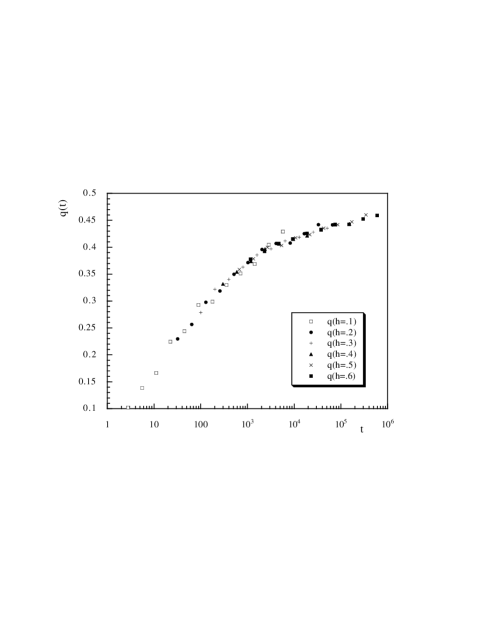
FIG. 4.: Rescaled functions $q(t)$ versus annealing time.

In figure (4) we show the rescaled functions (horizontal and vertical scales are given by the fact that we have kept fixed the values at $h=0.2$). The scaling is obeyed remarkably well: it works over six time decades, and in a range of magnetic fields going from $.1$ to $.6$. The errors on data point are not plotted since they would blur the figure. They are of the order of $0.01$-$0.02$. For example the point at $h=0.1$ with largest $t$ values, that is slightly out of the enveloping curve, is statistically compatible with the other points. $A$ and $B$ determined with the fits of figure (4) can now be fitted with power laws. We plot them in figure (5), with $A$ represented by the upper points and $B$ from the lower ones, together with the best fits (the fitting function are normalized in such a way to give $1$ at $h=0.6$). The best fit gives $A(h)\simeq 1.14(1)h^{.25(1)}$, and $B(h)\simeq 5.4(3)h^{3.3(1)}$. Even if this is a qualitative test, since we have only a rough estimate from the mean field approach, and in this case we have not analyzed the statistical and systematic error in great detail (since systematic error could be quite large for this measurement) the agreement with the values one would expect from the mean field solution turns out to be remarkably good.

We acknowledge useful discussions with C. Naitza, F. Ricci-Tersenghi and J. J. Ruiz-Lorenzo. We warmly thank F. Ritort for interesting correspondence and comments.

FIG. 5.: $A$ and $B$ from our best fit versus $h$.

REFERENCES

- [1] M. Mezard, G. Parisi and M. Virasoro, Spin Glass Theory and Beyond (World Scientific, Singapore 1987).
- [2] G. Parisi, preprint cond-mat/9603101; F. Guerra, Int. J. Mod. Phys. B 10, 1675 (1996).
- [3] C. M. Newman and D. L. Stein, Phys. Rev. Lett. 76, 515 (1996) ; C. M. Newman and D. L. Stein, preprint adap-org/9603001.
- [4] D. Iniguez, G. Parisi and J. Ruiz-Lorenzo, J. Phys. A 29, 4337 (1996).
- [5] E. Marinari, G. Parisi and J. Ruiz-Lorenzo, preprint cond-mat/9701016, to appear in Spin Glass and Random Fields, edited by P. Young.
- [6] E. Marinari, G. Parisi, F. Ritort, J. Phys. A 27, 2687 (1994); E. Marinari, G. Parisi, F. Ritort and J. Ruiz-Lorenzo, Phys. Rev. Lett. 76, 843 (1996); N. Kawashima and P. Young, Phys. Rev. B 53, 484 (1996); A. Cacciuto, E. Marinari and G. Parisi, preprint cond-mat/9608161; G. Parisi, P. Ranieri, F. Ricci-Tersenghi and J. Ruiz-Lorenzo, preprint cond-mat/9702030.
- [7] J. R. L. de Almeida and D. J. Thouless, J. Phys. A 11, 11 (1978).
- [8] S. Caracciolo, G. Parisi, S. Patarnello and N. Sourlas, Europhys. Lett. 11, 783 (1990); J. Phys. France 51, 1877 (1990); E. R. Grannan and R. E. Hetzel, Phys. Rev. Lett. 67, 907 (1991); J. C. Ciria, G. Parisi, F. Ritort and J. Ruiz-Lorenzo, J. Phys. I France 3, 2207 (1993); M. Picco and F. Ritort, J. Phys. I France 4, 1619 (1994); J. O. Andersson, J. Mattsson and P. Svedlindh, Phys. Rev. B 49, 1120 (1994).
- [9] M. Picco and F. Ritort, preprint cond-mat/9702041.
- [10] F. Zuliani, to be published.
- [11] E. Marinari, C. Naitza and F. Zuliani, to be published.
- [12] G. Parisi, F. Ricci-Tersenghi and J. Ruiz-Lorenzo, J. Phys. A 29, 7943 (1996).
- [13] G. Parisi, J. Vannimenus and G. Toulouse, J. de Physique 42, 565 (1981).