Trapping and Wiggling: Elastohydrodynamics of Driven Microfilaments

Abstract

We present a general theoretical analysis of semiflexible filaments subject to viscous drag or point forcing. These are the relevant forces in dynamic experiments designed to measure biopolymer bending moduli. By analogy with the “Stokes problems” in hydrodynamics (fluid motion induced by that of a wall bounding a viscous fluid), we consider the motion of a polymer one end of which is moved in an impulsive or oscillatory way. Analytical solutions for the time-dependent shapes of such moving polymers are obtained within an analysis applicable to small-amplitude deformations. In the case of oscillatory driving, particular attention is paid to a characteristic length determined by the frequency of oscillation, the polymer persistence length, and the viscous drag coefficient. Experiments on actin filaments manipulated with optical traps confirm the scaling law predicted by the analysis and provide a new technique for measuring the elastic bending modulus. A re-analysis of several published experiments on microtubules is also presented.

]

I Introduction

The attempts of theoretical physicists to contribute in some useful way to the study of biology has, so far, been most successful in systems in which all forces and motion can be modeled and mathematized explicitly, or those governed by equilibrium statistical mechanics, for which equipartition can be invoked. One specific example of this success is the analysis of structural microfilaments, essentially one-dimensional mechanical objects with no moving parts. Despite this unassuming mechanical description, these semiflexible biopolymers are responsible for innumerable essential functions at the molecular and cellular level.

Depending on the bending modulus of the filament in question, experiments on semiflexible biopolymers largely rely on either mechanical or statistical techniques. Microtubules, with a persistence length $\sim 5$ mm, are quite amenable to micromanipulation or forcing via hydrostatic drag. Actin and nucleic acids, with persistence lengths near $15\mu$ and $50$ nm, respectively, fall in the realm of statistical mechanics (note that we are here addressing the bending elasticity, not the stretching elasticity, another area of great excitement and successes [37, 5, 30]).

However, much of the analysis of elasticity in this context seems to ignore a fact known to the ancients who developed the field: boundaries matter for finite objects. While often in physics boundary effects can be ignored, the fact that biopolymers are finite has important and unexpected consequences and must be included carefully the analysis. These effects appear because dynamics of the elastica are governed by fourth-order spatial derivatives. This fact forces us to rethink what are the most appropriate basis functions in which to model dynamics. While this question may seem purely academic, we will see that it is quite crucial in attempts to develop accurate dynamic methods for the quantitative study of semiflexible biopolymers

Specifically, we couple elasticity theory and overdamped viscous hydrodynamics (as is appropriate in the biological context) to explore elastohydrodynamics. While experiments coupling elasticity and drag have been presented before [10, 33], treatments of dynamics, rather than mechanical equilibrium, have been less than complete. Although equations with the appropriate units will be sufficient to determine the scales of forces and velocities, if we wish to extract numbers from the experiments it is necessary to have a thorough analysis. The slenderness of the filaments allows us greatly to simplify the hydrodynamics and arrive at a local partial differential equation of motion. Moreover, we will find that coupling to hydrodynamics allows us to extend the range of mechanical experiments to much smaller bending moduli. For example, whereas measurements of actin’s rigidity so far have been via fluctuation analyses invoking equipartition and thus statistical mechanics, we present here an experimental method which does not rely on nonzero temperature. Further, the method allows investigation into questions which have been raised as to whether or not actin can even be treated as a semiflexible polymer, or is in fact scale-sensitive [16] or dynamic in its elasticity. Such a purely mechanical treatment obviates possible complications to statistical treatments like dimensionality [26], correlations among sampled images, or self-avoidance.

It is our hope that this new experimental method, as well as the general analytic techniques here outlined, will contribute to the current exciting and active dialogue among physicists and biologists regarding the nature and numbers behind biopolymer rigidity as well as the effects of varying proteins and environments on elastic moduli. Further, these new methods and analyses should prove useful in the study of other examples of dynamic elastic filaments, such as supercoiled fibers of B. subtilis [24]. We intend this investigation to be the necessary starting point for such exciting extensions.

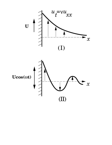
FIG. 1.: Geometry of Stokes problems I and II.

A useful starting point for developing the general mathematical treatment of the dynamics of an elastic filament in a viscous medium will be to consider the simplest time dependencies possible. To that end, recall the classic problems introduced by G.G. Stokes in 1851 [31], illustrated in Fig. 1, involving the motion of a viscous fluid bounded by a wall that is either (I) moved impulsively or (II) oscillated. These easily-solvable problems capture the essential ideas of viscous diffusion of velocity. The experimental geometry is such that the Navier-Stokes equation for the velocity field $u(x,t)$ is simply the diffusion equation

$$u_{t}=\nu u_{xx}~{},$$ (1)

where $\nu=\mu/\rho$ is the kinematic viscosity, and $\mu$ and $\rho$ are the fluid viscosity and density. Subscripts on functions will indicate differentiation throughout unless otherwise indicated. The salient features of the solutions are the relationships between length scales, time scales, and material parameters. Specifically, in the impulsive case, the velocity at any point $x$ and time $t$ depends only on the ratio $x/(\nu t)^{1/2}$; likewise, in the oscillatory case, oscillations decay with a characteristic length that scales as $\ell_{S}(\omega)=({\nu/\omega})^{1/2}$.

We introduce here the analogous two problems in elastohydrodynamics, illustrated in Fig. 2. They involve (I) the deflection of a polymer anchored at one end following the instantaneous introduction of a uniform fluid velocity $U$, and (II) the steady undulations of a polymer one end of which is oscillated. Rather than a diffusion equation as in the Stokes problems, the dynamics of small deformations $y(x,t)$ of the filament are governed by a fourth-order PDE of the form

$$y_{t}=-\tilde{\nu}y_{xxxx}~{},$$ (2)

where $\tilde{\nu}=A/\zeta$ plays the role of a “hyperdiffusion” coefficient, with $A$ the bending modulus and $\zeta$ the drag coefficient. This equation has appeared before in the literature on semiflexible biopolymers [1, 12], primarily in the context of scaling arguments for relaxation times; our goal here is to provide a complete solution given arbitrary initial and boundary conditions as dictated by experiment.

FIG. 2.: Geometry of elastohydrodynamic problems I and II.

An analysis similar to that presented below of the oscillatory passive elastica was carried out a number of years ago by K. E. Machin [22, 23], who considered the motion of a driven flagellum. Machin was interested specifically in a semiinfinite active flagellum which was bent with a set of boundary conditions amenable to analysis. Ours will be more malicious, but not subtle.

We will first derive the general equations of motion for elastica embedded in viscous flow. We then apply this dynamic to a number of scenarios. Inspired by “Stokes problems I and II” in fluid dynamics (SI and SII), we first solve “problems I and II” of elastohydrodynamics (EHDI and EHDII), each of whose dynamic mimics its hydrodynamic analogue. Problem I will require a bit of mathematical construction to assist our physical intuitions. Specifically, we must construct a set of basis functions appropriate to the equation of motion and specified boundary conditions. All the pleasant features found when applying Fourier space to unbounded or periodic systems are found here as well, in what we term ${\cal W}$-space. Unlike Fourier space, ${\cal W}$-space respects both the compact support and boundary conditions of the elastica and thus diagonalizes the equation of motion. We then discuss an experimental realization of problem II and its analysis, which provides a new technique for the measurement of a polymer’s bending modulus. Finally, we comment on some recent related experimental work by a separate group, brought to our attention as the original version of this paper was being completed.

II Elastic forces

A bent elastic polymer exerts a restorative force given by the functional derivative of a bending energy

$${\bf f}_{\cal E}=-{\delta{\cal E}\over\delta{\bf r}},$$ (3)

which for an elastic curve may be expressed as

$${\cal E}={1\over 2}A\int_{0}^{L}\!\!ds\kappa^{2}~{}.$$ (4)

Here, $A$ is the bending stiffness constant, with units of energy $\times$ length. It may also be expressed as the product $EI$ of the Young’s modulus $E$ and the moment of inertia $I$[11]. For a polymer of persistence length $L_{p}$ at absolute temperature $T$, exploring all configurations in $D$ dimensions, we may also derive by equipartition the equivalence $A=(D-1)k_{B}TL_{p}/2$.

Henceforth we will consider elastic filaments that lie in a plane. This is the geometry most well-suited to data-taking via microscopy. The curvature $\kappa$ may then be expressed exactly as $d{\theta}/ds$, where $\theta$ is the angle between the tangent to the curve and some fixed axis (see Fig. 3); the $x$-axis is a convenient choice, for which $\tan\theta=(dy/ds)/(dx/ds)=dy/dx$, which implies

$$\kappa={y_{xx}\over\left(1+y_{x}^{2}\right)^{3/2}}~{}.$$ (5)

Taking the functional derivative of the energy (4), we derive the force and boundary conditions

$${\bf f}_{\cal E}=A\left(\kappa_{ss}+{1\over 2}\kappa^{3}\right){\bf{\hat{n}}}~{},$$ (6)

$$\kappa=\kappa_{s}=0~{}~{}{\rm at~{}free~{}ends}.$$ (7)

These boundary conditions indicate the torquelessness and forcelessness, respectively, at free ends of an elastica [34]. At hinged or clamped ends different boundary conditions hold, as will be discussed below.

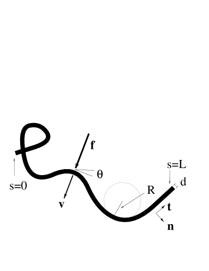
FIG. 3.: Geometry of an elastic filament: $R$=local radius of curvature; $\bf{t},\bf{n}$=unit tangent and normal, $\theta=\cos^{-1}({\bf{\hat{t}}}\cdot{\bf{\hat{e}}_{x}})$; $d$=diameter of the filament; arclength $s$ varies from $0$ to $L$, the total arclength. Within the approximations of slender-body hydrodynamics, a local anisotropic proportionality is satisfied between an external force per unit length $\bf f$ and the velocity $\bf v$.

We may linearize these results for small deviations from a horizontal line, ($y_{x}\ll 1$) or equivalently linearize Eq. 4 to find $\kappa\simeq y_{xx}+{\cal O}\left(y_{x}^{2}\right)$ and

$${\bf f}_{\cal E}\simeq-Ay_{xxxx}{\bf{\hat{e}}_{y}}+{\cal O}\left(y_{x}^{2}\right)~{},$$ (8)

(where ${\bf{\hat{e}}_{y}}$ is the unit vector in the $y$ direction) with boundary conditions

$$y_{xx}=0~{}{\rm and}~{}y_{xxx}=0~{}~{}{\rm at~{}free~{}ends}.$$ (9)

The specification of the filament dynamics is complete upon definition of the hydrodynamic drag which balances ${\bf f}_{\cal E}$. We now turn to this problem.

III Slender-body hydrodynamics

We wish to consider experiments taking place on cellular biological scales, with typical lengths $L$ in microns, times $t$ in seconds, and dynamic viscosity $\mu$ that of water, in centipoise. The nondimensional parameter characterizing the hydrodynamic behavior, the Reynolds number, is $UL/\nu\sim L^{2}/t\nu\sim 10^{-8}/10^{-2}\sim 10^{-6}$. We are thus safely in the low-Reynolds number or ‘Stokesian’ regime. In this Aristotelian overdamped limit, forces balance velocities rather than accelerations. For a body whose length is much greater than its width, the well-developed set of calculations known as ‘slender-body hydrodynamics’ applies [17, 6, 7]. If this filamentous polymer has diameter $d$, length $L$, and an aspect ratio $d/L\ll 1$, we have the simplified, local, anisotropic proportionality between the drag force ${\bf f}_{d}$ and the velocity ${\bf r}_{t}$,

$${\bf f}_{d}=\zeta\left[{\bf{\hat{n}}}{\bf{\hat{n}}}+\beta{\bf{\hat{t}}}{\bf{\hat{t}}}\right]\cdot\left({\bf r}_{t}-{\bf u}\right).$$ (10)

Here, ${\bf f}_{d}\left(s\right)$ is a force per unit length exerted on the filament, and ${\bf{\hat{n}}}\left(s\right)$ and ${\bf{\hat{t}}}\left(s\right)$ are unit vectors in the normal and tangential directions at arclength $s$ along the polymer. The velocity of the polymer is denoted ${\bf r}_{t}\left(s\right)$, and ${\bf u}$ is any background velocity which may be present in the problem; the drag should be a function of the former relative to the latter. The anisotropy, evident when dragging a pencil through molasses, between motions parallel and perpendicular to a slender object’s long axis is embodied by the parameter $\beta$, which depends logarithmically on the aspect ratio, with asymptotic behavior

$$\lim_{d/L\rightarrow 0}\beta={1\over 2}~{}.$$ (11)

An active field of applied mathematics in the last twenty years has been calculations of the viscous drag coefficient $\zeta$ for various slender shapes [17, 6, 7, 20, 4, 29]. The limiting behavior for small $d/L$ has the form

$$\zeta={4\pi\mu\over{\ln\left(L/d\right)+c}}~{}.$$ (12)

where $c$ is a constant of order unity which depends on the shape of the body.

Now that we have defined the hydrodynamic drag, we demand that it balances elastic forcing (${\bf f}_{d}={\bf f}_{\cal E}$) to derive the equation of motion:

$$\zeta\left[{\bf{\hat{n}}}{\bf{\hat{n}}}+\beta{\bf{\hat{t}}}{\bf{\hat{t}}}\right]\cdot\left({\bf r}_{t}-{\bf u}\right)=A\left(\kappa_{ss}+{1\over 2}\kappa^{3}\right){\bf{\hat{n}}}.$$ (13)

Linearizing the expression for the drag (10) for nearly-straight polymers ($y_{x}\ll 1$), and noting that its tangential components are of order $y_{x}^{2}$, the dynamic reduces to

$$\zeta\left(y_{t}-u\right)=-Ay_{xxxx}~{}.$$ (14)

Here, $u\equiv{\bf u}\cdot{\bf{\hat{e}}_{y}}$. In the absence of any background flow,

$$y_{t}=-{\tilde{\nu}}y_{xxxx},$$ (15)

where ${\tilde{\nu}}=A/\zeta$ as in Eq. 2. This is the simplest linearized expression of elastohydrodynamics: elastic forces, characterized by a fourth spatial derivative, balance viscous drag. It shares many similarities with the diffusion equation (1), and may be thought of as “hyperdiffusion” of displacement in analogy with hyperviscosity.

IV Elastohydrodynamic problem I

Now that we have established the equation of motion appropriate to these elastohydrodynamic analogs, we recall the solutions to the fluid dynamics problems SI and SII in hopes of exploiting the analogy as much as possible. In Stokes I (SI), a semiinfinite plane of fluid is forced by a wall which is motionless for time $t<0$ and has velocity $U{\bf{\hat{e}}_{y}}$ for $t>0$. In Stokes II (SII), the wall oscillates as $U\cos\left(\omega t\right){\bf{\hat{e}}_{y}}$, and we solve for the behavior after transients have died away.

As illustrated in Fig. 1, velocity gradients are in the $x$-direction in both cases, and hence perpendicular to the direction of flow (along the $y$-axis). In the absence of an imposed pressure gradient, the Navier-Stokes equation for the fluid velocity $u\left(x,t\right)$ parallel to the wall is simply the linear diffusion equation (1), $u_{t}=\nu u_{xx}$.

A convenient method of solving SI with the associated boundary condition is to postulate a scaling solution inspired by dimensional analysis: $u\left(x,t\right)=UF\left(\xi\right)$, with $\xi=x/\left(\nu t\right)^{1/2}$. The scaling function $F$ then obeys a nonautonomous ordinary differential equation

$$-{1\over 2}\xi F_{\xi}=F_{\xi\xi}~{}.$$ (16)

The solution to this is $F={\rm erfc}\left(\xi/\sqrt{2}\right)$, where ${\rm erfc}$ is the complementary error function. The dedicated may arrive at the same result more laboriously via Laplace transforming Eq. 1.

Armed with some understanding of SI, we now turn to problem I of elastohydrodynamics (EHDI). In problem I, we consider an elastic filamentous polymer which is anchored at the origin. For $t<0$ it lies along the line segment $\{y=0;\ 0<x<L\}$. We then may consider forcing the filament by moving one end relative to the fluid (moving the anchor) or moving the fluid relative to the polymer (moving, for example, the cover slip). We will first attempt to do this in a way as analogous to SI as possible.

A Semiinfinite polymer

Consider first moving the anchor relative to the fluid with velocity ${\bf u}=u{\bf{\hat{e}}_{y}}$. This may be thought of as moving a bead optically trapped to one end, or some other micromanipulation. We now observe that the equation of motion, $y_{t}=-{\tilde{\nu}}y_{xxxx}$, inspires a scaling solution of the form $y=utF\left(\xi\right)$, where $\xi\equiv x/\left({\tilde{\nu}}t\right)^{1/4}$. Inserting this special form of the solution, the equation becomes

$$F-{1\over 4}\xi F_{\xi}=-F_{\xi\xi\xi\xi},$$ (17)

an equation not unlike Eq. 16.

The solution $F$ must admit the conditions that it and its derivatives approach $0$ for a fixed time as $x\rightarrow\infty$, so

$$\lim_{\xi\rightarrow\infty}\{F\left(\xi\right),F_{\xi}\left(\xi\right),F_{\xi\xi}\left(\xi\right),\ldots\}=0~{}.$$ (18)

Moreover, specifying the anchor position implies

$$ut=y\left(0,t\right)=utF\left(0\right)~{}~{}\Rightarrow~{}~{}F\left(0\right)=1~{}.$$ (19)

Depending on whether we wish to describe a filament anchored by, for example, an axoneme or a bead, we demand $y_{x}\left(0\right)=0$ or $y_{xx}\left(0\right)=0$, implying $F_{\xi}(0)=0$ or $F_{\xi\xi}\left(0\right)=0$, respectively.

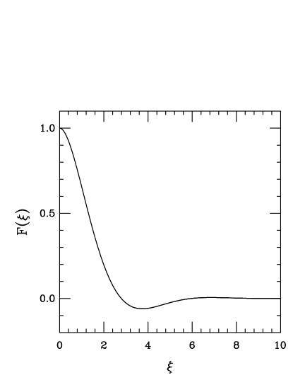
FIG. 4.: Scaling solution to (1) for a semiinfinite clamped polymer. The meaning of “scaling solution” is that $y$, $x$, and $t$, are suitably rescaled such that, if a friend were to imprint this image on silly putty, and run towards you with a velocity $\sim t^{-5/4}$ while stretching the putty in the $y$ direction a length $\sim t^{3/4}$, you would see the predicted shape of the semiinfinite elastica. For the most accurate results, have your friend start infinitely far away. This complication is obviated by considering the finite elastica.

Note that, had we instead chosen to consider a fixed anchor and a moving fluid, we would merely implement two changes. First, the equation of motion becomes $\left(y_{t}-u\right)=-{\tilde{\nu}}y_{xxxx}$. Second, the boundary condition becomes $y\left(0\right)=0$. However, introducing a Galilean change of frame $y^{\prime}\left(x,t\right)=y-ut$, we see that we recover the equivalent equation of motion, boundary conditions, and thus problem. This relationship between boundary conditions and equations of motion will allow us to apply one analysis to a number of experiments. We will use the terms “homogeneous” and “inhomogeneous” referring to both boundary conditions and equations of motions since we may transform from one to the other so simply.

Though nonautonomous, Eq. (17) is linear in $F$ and quite amenable to numerical solution. A plot of the solution for the clamped ($y_{x}(0)=0$) polymer is shown in Fig. 4. Clearly, the function satisfies our qualitative intuitions about the shape: an initially straight curve slopes towards $0$ as the argument grows, where all derivatives vanish. The appearance of the wiggle leads us more carefully to consider the realm of validity of our solution. Given our scaling ansatz $y=utF(\xi)$, we see that the slope $y_{x}=utF_{\xi}/({\tilde{\nu}}t)^{1/4}$ grows in time without bound, thus failing to meet the criterion on which the linearization of Eq. 13 was predicated: $y_{x}\ll 1$. Intuitively, we suspect that the neglected nonlinear terms would suppress these undulations.

Noting that $|F_{\xi}|$ attains its largest value of $\simeq 0.51$ for $\xi^{*}\simeq 1.1$, we see that we can only trust the solution to initial times such that

$$t\ll{{\tilde{\nu}}^{1/3}\over\left(uF_{\xi}\left(\xi^{*}\right)\right)^{4/3}}\simeq 2.5{\left({{\tilde{\nu}}/u}\right)^{1/3}\over u}$$ (20)

For an experimentally convenient velocity of $\sim 10\mu/s$, this time is order a fraction of a second for actin, and a second for microtubules. We have thus seen that the obvious extension of the hydrodynamic analogue is not necessarily the correct approach – a conclusion which will be reached repeatedly in this investigation.

Enjoyable though it is to contemplate the long-time behavior of the semiinfinite dragged elastica, a more profitable inquiry would be the experimentally realizable case of a finite polymer. We therefore turn now to the case of the finite elastica, clamped at one end and free at the other, and subject to impulsive hydrodynamic drag. Our analysis is applicable to experiments in which either the cover slip is moved or, as a special case, in which the elastica is allowed to relax from some initial conditions in the absence of flow.

B Finite polymer

In order to make the mathematics as transparent as possible, we first nondimensionalize the equation of motion (14). Distances in $x$ are rescaled by the total length $L$, time by the elastohydrodynamic time scale $\zeta L^{4}/A$, and distances in $y$ by the velocity times this time scale:

$$x=\alpha L~{},\ \ \ t=\tau{\zeta L^{4}\over A},\ \ \ y\left(x,t\right)=u{\zeta L^{4}\over A}h\left(\alpha,\tau\right)~{}.$$ (21)

The governing equation, $(y_{t}-u)=-{\tilde{\nu}}y_{xxxx}$, then becomes

$$(h_{\tau}-1)=-h_{\alpha\alpha\alpha\alpha}~{}.$$ (22)

Like any other inhomogeneous differential equation, the general solution of (22) must be the homogeneous solution ($h_{\tau}=-h_{{\alpha\alpha\alpha\alpha}}$) plus the particular solution ($h_{\tau}-1=-h_{{\alpha\alpha\alpha\alpha}}$). We indicate this by defining

$$h=f+g$$ (23)

where $g$ and $f$ satisfy

$${g}_{\tau}=-g_{{\alpha\alpha\alpha\alpha}},~{}~{}~{}{f}_{\tau}-1=-f_{{\alpha\alpha\alpha\alpha}}.$$ (24)

We will find that these two functions have markedly different qualitative behavior.

1 Homogeneous solution

The homogeneous equation is ${g}_{\tau}=-g_{{\alpha\alpha\alpha\alpha}}$. Well-versed in the litany of Fourier transforms, we first left-multiply by an as-yet arbitrary function ${\cal W}_{k}\left(\alpha\right)$ (where $k$ indicates a parameter rather than a derivative) and integrate over the domain of $\alpha$,

$$\int_{0}^{1}\!d\alpha{\cal W}_{k}{\partial_{\tau}g}=-\int_{0}^{1}\!d\alpha{\cal W}_{k}\partial_{\alpha}^{4}g~{}.$$ (25)

Integrating by parts we obtain

$$\partial_{\tau}\int_{0}^{1}\!d\alpha{\cal W}_{k}g =- \int_{0}^{1}d\alpha\partial_{\alpha}^{4}({\cal W}_{k})g$$ (26)

$$- {\cal W}_{k}\partial_{\alpha}^{3}g\bigl{|}_{0}^{1}+\partial_{\alpha}^{1}{\cal W}_{k}\partial_{\alpha}^{2}g\bigl{|}_{0}^{1}$$ (27)

$$- \partial_{\alpha}^{2}{\cal W}_{k}\partial_{\alpha}^{1}g\bigl{|}_{0}^{1}+\partial_{\alpha}^{3}{\cal W}_{k}g\bigl{|}_{0}^{1}.$$ (28)

Observe that the integration by parts of the fourth-order derivative introduces $8$ separate surface terms. The boundary conditions implied by the functional derivative (7) dictate the vanishing of the second and third derivatives at the free end ($x=L$). Requiring $g$ to satisfy this condition eliminates two of the $8$ terms.

The left end of the polymer is clamped at the origin, so $y\left(x=0\right)=y_{x}\left(x=0\right)=0$. Demanding this behavior of $g$ eliminates two additional surface terms. We now choose ${\cal W}_{k}$ to satisfy the same boundary conditions as $y$ and $g$, and therefore $h$:

$${\cal W}_{k}\left(0\right)=0 ,~{}~{}\partial_{\alpha}{\cal W}_{k}\left(0\right)=0,$$ (29)

$$\partial^{2}_{\alpha}{\cal W}_{k}\left(1\right)=0 ,{}~{}\partial^{3}_{\alpha}{\cal W}_{k}\left(1\right)=0.$$ (30)

This annihilates the remaining 4 surface terms in (28). Finally, we choose ${\cal W}_{k}$ to obey

$$\partial_{\alpha}^{4}{\cal W}_{k}=k^{4}{\cal W}_{k}~{}.$$ (31)

Defining $g_{k}\equiv\int_{0}^{1}\!d\alpha{\cal W}_{k}g~{},$ the equation of motion becomes ${\partial_{\tau}g_{k}}=-k^{4}g_{k},$ the solution to which is

$$g_{k}\left(\tau\right)=g_{k}\left(0\right){\rm e}^{-k^{4}\tau}~{}.$$ (32)

If we wish to describe the dynamics in such terms, we must construct the ${\cal W}_{k}$, which necessitates that we identify the allowed values of $k$. We turn now to this problem.

2 Explicit construction of the ${\cal W}_{k}$

A moment’s thought reveals that the ${\cal W}_{k}$ can not be constructed out of simply the familiar sin’s and cos’s of Fourier space, which are incompatible with boundary conditions in which successive derivatives vanish (cf.  Eq. 7). A countably infinite family of such ${\cal W}_{k}$ can, however, be constructed by including hyperbolic functions as well in the basis of the function space. The general solution of Eq. 31 is

$${\cal W}_{k}=a_{1} \sin\left(k\alpha\right) +a_{2}\cos\left(k\alpha\right)$$ (33)

$$+a_{3} \sinh\left(k\alpha\right) +a_{4}\cosh\left(k\alpha\right).$$ (34)

The expression has four unknowns, as a solution to a fourth-order problem must. The $\alpha=0$ (left end) boundary conditions yield $a_{4}=-a_{2}$ and $a_{3}=-a_{1}.$ The last two conditions, $\partial_{\alpha}^{2}{\cal W}_{k}\left(1\right)=0$ and $\partial_{\alpha}^{3}{\cal W}_{k}\left(1\right)=0$, can be expressed as a matrix equation

$$\pmatrix{\sinh k+\sin k&\cosh k+\cos k\cr\cosh k+\cos k&\sinh k-\sin k}\pmatrix{a_{1}\cr a_{2}}=0.$$ (35)

Since the matrix has a zero eigenvalue, it must be singular. This solvability condition is

$$\cos k=-{1\over\cosh k}~{}.$$ (36)

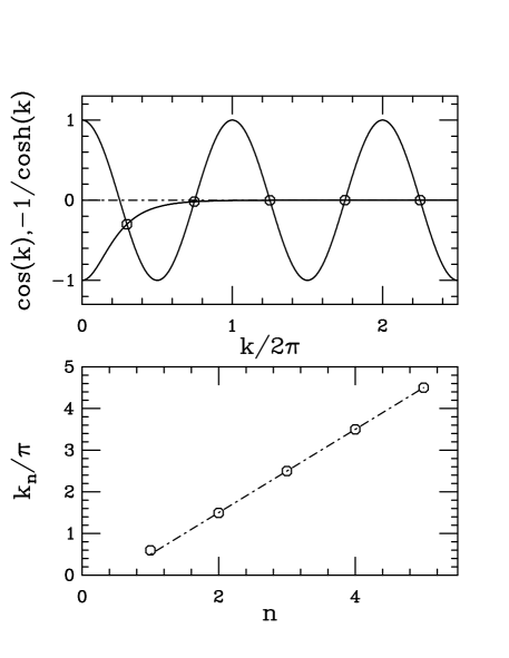
FIG. 5.: Solution of the transcendental equation for the roots $k_{n}$. (a) Graphical construction of the solution. (b) The roots (circles) asymptote to $k_{n}=\pi\left(2n-1\right)/2$ (dashed line).

As Fig. 5 illustrates, this transcendental equation has an infinite number of solutions. For large values of $k$, as $1/\cosh k\rightarrow 0$, the solutions approach the solutions of the Fourier-like solvability condition $\cos k=0$, i.e.,  $k_{n+1}\rightarrow{\pi\over 2}+\pi n$. The first few solutions are

$$k_{1} \simeq{\pi\over 2}+.304\simeq 1.875~{}, k_{2}\simeq{3\pi\over 2}-.018\simeq 4.694~{},$$ (37)

$$k_{3} \simeq{5\pi\over 2}+.001\simeq 7.855,~{} k_{4}\simeq{7\pi\over 2}\simeq 10.996~{},\ldots$$ (38)

We can insert either row of the LHS of (35) to solve for the relationship between $a_{2}$ and $a_{1}$, which we will express here as

$$a_{2}=-\left({\sin k+\sinh k\over\cos k+\cosh k}\right)a_{1}.$$ (39)

The constants themselves are functions of $k$. Note also that as $k\rightarrow\pm\infty$, $a_{2}\rightarrow\pm 1$. We now choose $a_{1}$ such that ${\cal W}_{k}$ is normalized, i.e., $\int_{0}^{1}d\alpha{\cal W}_{k}^{2}=1$. The first three eigenfunctions are shown in Fig. 6.

We have now completely and explicitly constructed the family of functions ${\cal W}_{k}$ which are normalized eigenfunctions of $\partial_{\alpha}^{4}$ with particular boundary conditions. Note that had we chosen some other set of boundary conditions, a different solvability condition and eigenfamily would have resulted (cf. Appendix A). For example, in the case of the elastica with free ends, we employ an expansion of $y$ with the basis functions of Eq. (A8). Note that if we differentiate this expression and define $\alpha_{n}=k_{n}/2$, then we recover Eq. 28 of [12]. The expansion in terms of $k$ has the advantage of a single solvability condition $\cos(k_{n})\cosh(k_{n})=1$, rather than the two conditions $\tanh(\alpha_{n})=(-1)^{n}\tan(\alpha_{n})$. The latter two conditions may be derived from the former via half-angle formulae.

This operator is self-adjoint (cf. Appendix B) and thus the eigenfunctions constitute a complete basis in function space onto which we may project initial data and relate to later-time solutions via Eq. 32 in the standard Green’s function way:

$$g\left(\alpha,\tau\right) = \sum_{k}|{\cal W}_{k}\rangle\langle{\cal W}_{k}|g\left(\alpha,\tau\right)\rangle$$ (40)

$$= \sum_{k}|{\cal W}_{k}\rangle g_{k}\left(0\right){\rm e}^{-k^{4}\tau}$$ (41)

$$= \int_{0}^{1}\!d\alpha^{\prime}{\cal G}\left(\alpha,\alpha^{\prime};\tau\right)g\left(\alpha^{\prime},0\right)~{},$$ (42)

where the Green’s function is

$${\cal G}(\alpha,\alpha^{\prime};\tau)=\sum_{k}{\cal W}_{k}\left(\alpha\right){\cal W}_{k}\left(\alpha^{\prime}\right){\rm e}^{-k^{4}\tau}{}.$$ (43)

This is the exact solution of the linearized homogeneous equation. Note that the compact support and the boundary conditions break translation invariance, reflected in the fact ${\cal G}$ can not be expressed as ${\cal G}\left(\alpha-\alpha^{\prime};\tau\right)$.

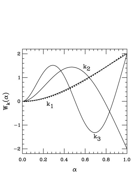
FIG. 6.: The first three eigenfunctions for EHD problem I. The dotted line indicates the normalized third-order polynomial describing an elastica bent by a point force at the right end. Note the surprising overlap with ${\cal W}_{k_{1}}$, as will be exploited in section VII A.

We note from the exact solution (43) that each mode $g_{k}$ decays independently and exponentially with time. This is to be compared with diffusive problems, in which each mode decays exponentially in time, except for the zero (average) mode, which is constant. In this experiment, the boundary conditions are incompatible with the existence of a zero mode. The system “hyperdiffuses” to homogeneity.

3 Particular solution

Since $g(\alpha,\tau)$ decays to zero as $\tau\to\infty$, we have

$$\lim_{\tau\rightarrow\infty}h\left(\alpha,\tau\right)=f\left(\alpha,\infty\right).$$ (44)

Thus the particular solution, if it exists, must be the long-time solution; no matter what initial data, the solution to the inhomogeneous equation of motion (22) must be the global attractor.

By the same argument, we must only construct a solution for it to be the correct one. We first look for a time-independent function, for which Eq. 24 becomes $1=f_{\alpha\alpha\alpha\alpha}$. The unique solution consistent with the boundary conditions (30) is

$$f\left(\alpha\right)={1\over 24}\left(\alpha^{4}-4\alpha^{3}+6\alpha^{2}\right)\equiv{\bar{h}}\left(\alpha\right)$$ (45)

4 Digression on boundary conditions

It is useful to pause momentarily and reflect on the importance of boundary conditions and how they will enter into the analysis. To this end, we consider an analogous experiment in which the left side of the polymer is hinged rather than clamped. This would be realized by holding the polymer in an optical trap, for example, rather than some torque-exerting anchor like an axoneme fixed to a cover slip. For this experimental setup we replace the boundary condition $h_{\alpha}\left(0,\tau\right)=0$ with $h_{\alpha\alpha}\left(0,\tau\right)=0$.

Intuitively, we expect the polymer to align itself with the flow as $t\rightarrow\infty$ in the absence of any torque at the left end. Mathematically, we may think of the change in boundary conditions via some curious pathologies. The first complication is that there does not exist a time independent fourth-order polynomial in $\alpha$ which is consistent with the boundary conditions. This prevents us from constructing a static attractor for the problem. However, we note that the equation of motion is solved by a fifth-order, time-dependent polynomial in $\alpha$:

$${\bar{h}}\left(\alpha,\tau\right)={3\over 2}\left(\tau+C\right)\alpha+{1\over 4!}\left(-\alpha^{3}+\alpha^{4}-{3\over 10}\alpha^{5}\right).$$ (46)

To derive this poynomial, we first express the solution in the form $\sum_{n}c_{n}\left(\tau\right)\alpha^{n}$. However, we are considering a Stokesian dynamic, in which the time dependence is first-order and the equation of motion is linear; the driving is a constant in time and thus time should enter only linearly into any steady state solution for the position (cf. [19]). Constraining $\partial_{t}^{2}c_{n}=0$ and respecting the relationship between $\partial_{\tau}c_{n}$ and $c_{n+4}$ dictated by Eq. 22, we uniquely specify the polynomial up to the constant $C$.

The fact that our long-time solution has an arbitrary constant should lead us to rethink splitting the solution into a polynomial and a set of only-decaying modes. Returning to the set of eigenvalues of $\partial_{\alpha}^{4}$, we discover a second complication for this new boundary condition: there now exists a zero mode – a nontrivial solution, consistent with the boundary conditions, to the equation $\partial_{\alpha}^{4}{\cal W}_{0}=0$, i.e.,  the normalized polynomial $\sqrt{3}\alpha$. We then may choose $C$ to eliminate the overlap of ${\cal W}_{0}$ with the initial data, i.e.,  $0=g_{0}=\langle g|{\cal W}_{0}\rangle=\langle h(\alpha,0)|{\cal W}_{0}\rangle-\langle{\bar{h}}(\alpha)|{\cal W}_{0}\rangle$.

We now see how the change in boundary conditions creates drastically different physical behavior. The long-time solution contains a term describing a straight line whose slope grows with velocity $3u/2L$ without bound.

In order further to illustrate the relationship between a change in boundary conditions and the qualitative behavior, note that the dynamics, even in the presence of an inhomogeneous equation of motion, can be cast in terms of the functional derivative of an energy:

$${h}_{\tau} = -{\delta{\cal F}\over\delta h\left(\alpha\right)},$$ (47)

$${\cal F} = \int_{0}^{1}\!d\alpha^{\prime}\left[-h+{1\over 2}\left(h_{\alpha\alpha}\right)^{2}\right].$$ (48)

The first term represents the drag force acting in the positive $y$ direction, while the second is simply the nondimensionalization of the elastic bending energy term from which we originally derived the equation of motion. We then find

$${{\cal F}_{\tau}}=\int_{0}^{1}d\alpha{h_{\tau}}{\delta{\cal F}\over\delta h\left(\alpha\right)}=-\int_{0}^{1}d\alpha\left(h_{\tau}\right)^{2},$$ (49)

indicating ${\cal F}$ is a monotonically decreasing function in time [8, 13].

We must now only show that for the clamped (hinged) polymer this energy functional is (is not) bounded from below. Rewriting $h=\sum c_{n}(\tau)\alpha^{n},$ we can evaluate the energy explicitly as

$${\cal F}=-\sum_{n=0}^{\infty}{c_{n}\over n+1}+{\cal R}~{},$$ (50)

where

$${\cal R}={1\over 2}\sum_{m,n=2}^{\infty}{n\left(n-1\right)m\left(m-1\right)\over n+m-3}c_{m}c_{n}~{}.$$ (51)

If $h\left(0\right)=h_{x}(0)=0$, $c_{0}=c_{1}=0$. Eq. 50 then becomes

$${\cal F}=-\sum_{n=2}^{\infty}{c_{n}\over n+1}+{\cal R}~{}.$$ (52)

We see that we can not simply make the first term arbitrarily negative by introducing a large and positive $c_{j}$ for some $j$, since this term will appear quadratically (and always positively) in the second term. However, replacing the condition $h_{\alpha}\left(0\right)=0$ with $h_{\alpha\alpha}\left(0\right)=0$ changes the condition $c_{1}=0$ to $c_{2}=0$, and the energy becomes

$${\cal F}=-{c_{1}\over 2}-\sum_{n=3}^{\infty}{c_{n}\over n+1}+{\cal R}~{}.$$ (53)

Now the energy can become arbitrarily negative if $c_{1}=h^{\prime}(0)$ becomes arbitrarily positive. A divergent slope simply means the curve points straight up, in accord with our intuition for the long time behavior of a polymer free to rotate in some background flow. Note such a long-time behavior means leaving the small-$h_{x}$ limit for which the dynamic was originally derived.

5 General solution

Returning to the clamped polymer in the presence of some background flow, we project the definitional statement $h\left(\alpha,\tau\right)=g\left(\alpha,\tau\right)+{\bar{h}}\left(\alpha\right)$ onto the ${\cal W}_{k}\left(\alpha\right)$:

$$h_{k}\left(\tau\right)=g_{k}\left(\tau\right)+{\bar{h}}_{k},$$ (54)

which implies the initial condition $g_{k}\left(0\right)=h_{k}\left(0\right)-{\bar{h}}_{k}$. Recalling the simple time-dependence of the modes $g_{k}$ from Eq. (32), we see

$$h_{k}\left(\tau\right)={\bar{h}}_{k}\left(1-{\rm e}^{-k^{4}\tau}\right)+h_{k}\left(0\right){\rm e}^{-k^{4}\tau}.$$ (55)

The dynamic thus mimics that of a capacitor, charging up with the final shape-state and draining of the initial shape-state, each mode governed independently with decay rate $k^{-4}$. In real space,

$$h\left(\alpha,\tau\right) = {\bar{h}}\left(\alpha\right)+\sum_{k=k_{1}}^{\infty}{\cal W}_{k}\left(\alpha\right){\rm e}^{-k^{4}\tau}$$ (57)

$$\times\int_{0}^{1}\!d\alpha^{\prime}{\cal W}_{k}\left(\alpha^{\prime}\right)\left[h\left(\alpha^{\prime},0\right)-{\bar{h}}\left(\alpha^{\prime}\right)\right].$$

In the experiment considered, the initial condition is a flat polymer: $h\left(\alpha,\tau=0\right)=0$. Since ${\bar{h}}$ is the solution to ${\bar{h}}_{\alpha\alpha\alpha\alpha}=1$, with boundary conditions ${\bar{h}}\left(0\right)={\bar{h}}_{\alpha}\left(0\right)={\bar{h}}_{\alpha\alpha}\left(1\right)={\bar{h}}_{\alpha\alpha\alpha}\left(1\right)=0$, we find upon integrating by parts that

$$\int_{0}^{1}d\alpha^{\prime}{\cal W}_{k}\left(\alpha^{\prime}\right){\bar{h}}\left(\alpha^{\prime}\right)={{\bar{\cal W}_{k}}\over k^{4}}~{},$$ (58)

where ${\bar{\cal W}_{k}}\equiv\int_{0}^{1}d\alpha{\cal W}_{k}$, and thus Eq. 57 reduces to

$$h\left(\alpha,\tau\right)={\bar{h}}\left(\alpha\right)-\sum_{k=k_{1}}^{\infty}{\cal W}_{k}\left(\alpha\right){{\bar{\cal W}_{k}}\over k^{4}}{\rm e}^{-k^{4}\tau}{}.$$ (59)

Evaluating the first few integrals, we find for ${\bar{h}}_{k}\equiv\int d\alpha{\cal W}_{k}{\bar{h}}={\bar{\cal W}_{k}}/k^{4}$,

$${\bar{h}}_{k_{1}} \simeq 6\times 10^{-2}~{},\ \ \ {\bar{h}}_{k_{2}}\simeq 9\times 10^{-4}~{},\ \ \ {\bar{h}}_{k_{3}}\simeq 7\times 10^{-5}~{},$$ (60)

$${\bar{h}}_{k_{4}} \simeq 1\times 10^{-5}~{}\ \ \ \ldots$$ (61)

Each mode with $k>k_{1}$ decays exponentially faster in time than the lowest mode, which thus dominates as $\tau\rightarrow\infty$, so

$$h\rightarrow{\bar{h}}(\alpha)-{\bar{h}}_{k_{1}}{\rm e}^{-k_{1}^{4}\tau}\simeq{\bar{h}}-0.06{\cal W}_{k_{1}}{\rm e}^{-12.36\tau}.$$ (62)

Our picture of the impulsive dynamic of elastica in viscous flow is thus as follows: we project onto a special function space in which the long-time solution and the difference between initial data and the long-time solution exponentially charge and decay, respectively, each mode behaving independently. We are left with only the the long-time solution as the asymptotic limit $\tau\rightarrow\infty$.

V Elastohydrodynamic problem II

In Stokes II, the driving force is exerted by a wall oscillating with velocity ${\bf u}=U{\bf{\hat{e}}_{y}}\cos\left(\omega t\right)$, or position $y=y_{0}\cos\left(\omega t\right)$. To solve the steady-state limit of SII, we postulate $u\left(x,t\right)=U\Re\left(e^{i\omega t}G\left(\eta\right)\right)$, where $\eta=x{(\omega/\nu)}^{1/2}$. Inserting into Eq. 1, we then see $G$ satisfies

$$iG=G_{\eta\eta}~{},$$ (63)

for which the solution vanishing as $\eta\to\infty$ is $G={\rm e}^{-\sqrt{i}\eta}$. We then find $u\left(x,t\right)=U{\rm e}^{-\eta/\sqrt{2}}\cos\left(\omega t-\eta/\sqrt{2}\right)$, or, in a form useful for comparison to the elastohydrodynamic case,

$$u\left(x,t\right)=U{\rm e}^{-S_{4}\eta}\cos\left(C_{4}\eta-\omega t\right)$$ (64)

where $C_{4}=\cos(\pi/4)$ and $S_{4}=\sin(\pi/4)$. This solution describes right-moving waves of velocity $\omega\ell/C_{4}$, decaying as $x\rightarrow\infty$ with decay length $\ell/S_{4}$.

We now consider a polymer held by an optical trap which moves with position $y\left(x=0\right)=y_{0}\cos\left(\omega t\right)$. Since we have shown in the previous section that all modes satisfying the homogeneous equation of motion with homogeneous boundary conditions decay exponentially, we must only find a solution in the presence of inhomogeneity (here, the driving) to find the long-time limit of the dynamic.

In order to verify the validity of our analysis as well as the plausibility of EHDII as a method for measuring biopolymer rigidity, we conducted the experiment and analyzed image data as described below. A scaling relation predicted by the analysis was confirmed, and a new method for measurement of the persistence length of actin was demonstrated.

The experimental setup is shown in Fig. 7: F-actin is bound to a silica bead which is optically trapped. By oscillating the position of the bead sinusoidally in time, the filament wiggles back and forth, propagating waves of displacement down its length. The motion relative to the fluid is opposed by the fluid viscosity, and the “wiggles” are opposed by the elasticity of the polymer.

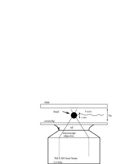
FIG. 7.: Experimental setup.

A The characteristic length

The elastic constant $A$ has units of ${\rm energy}\times{\rm length}$, while the viscous force per unit length per unit velocity has the dimensions of a viscosity or action density $\mu$:

$$[\zeta]=[\mu]={{\rm mass}\over{\rm length}\times{\rm time}}={{\rm energy}\times{\rm time}\over{\rm length}^{3}}~{}.$$ (65)

Thus, the natural length obtained from $A$, $\zeta$, and the frequency of oscillation $\omega$ is

$$\ell\left(\omega\right)=\left({A\over\omega\zeta}\right)^{1/4}=\left({k_{B}TL_{p}\over\omega\zeta}\right)^{1/4}.$$ (66)

Nota bene that $\ell(\omega)$ is not a mere rescaling of the persistence length.

With a previously-published persistence length for actin of $L_{p}\simeq 15\mu$m[26], a viscosity $\mu=0.01$ cp, $k_{B}T\simeq 4\times 10^{-14}$ erg at $T=300$ K, and measuring $\omega$ in units of sec^-1, we obtain

$$\ell\left(\omega\right)\simeq\left(2.8{\mu{\rm m}\over s^{1/4}}\right)\omega^{-1/4}.$$ (67)

Thus for frequencies on the order of $1$ Hz, we obtain length scales of order microns, somewhat below the persistence length. This range of frequencies seems quite advantageous for experiment.

This elastohydrodynamic length $\ell\left(\omega\right)$ is precisely the length found upon nondimensionalizing the equation of motion (15). By analogy to SII, we define the dimensionless coordinate $\eta=x/({\tilde{\nu}}\omega)^{1/4}=x/\ell(\omega)=x\left(A/\omega\zeta\right)^{-1/4}$ and rewrite the solution as

$$y\left(x,t\right)=y_{0}{\Re}\{{\rm e}^{i\omega t}h\left(\eta\right)\}~{}$$ (68)

and Eq. 2 as

$$ih(\eta)=-{\partial}_{\eta}^{4}h\left(\eta\right).$$ (69)

The solutions of (69) are of the form

$$h\left(\eta\right)=c{\rm e}^{\gamma\eta}$$ (70)

where $\gamma$ may be any one of the four distinct (complex) numbers such that $\gamma^{4}=-i$. These are

$$\gamma_{j}=i^{j}{\rm e}^{-i\pi/8}\ \ \ \ \ \ \ \left(j=1\ldots 4\right)~{}.$$ (71)

The general solution is the sum of these four solutions,

$$h\left(\eta\right)=\sum_{j=1}^{4}c_{j}{\rm e}^{i^{j}z_{0}\eta}~{},$$ (72)

where

$$z_{0}\equiv{\rm e}^{-i\pi/8}\simeq 0.92-0.38~{}i~{}.$$ (73)

The unpleasant (but certainly not subtle) remainder of the problem is to solve for the four $c_{j}$’s, given some four boundary conditions. At the left end, we enforce not only the position at $x=0$ but the condition of torquelessness, as appropriate for an optical trap, $y_{xx}(0)=0$. The right end must satisfy the free end boundary conditions, Eq. 9. The $c_{j}$ derived from these conditions are functions of a rescaled polymer length ${\cal L}\equiv L/\ell\left(\omega\right)$ and may properly be written as $c_{j}\left({\cal L}\right)$.

B Semiinfinite polymer

The exact solution for $h\left(\eta\right)$ is presented in Appendix C; it simplifies greatly, however, for extreme values of $L/\ell(\omega)$. In the limit of an infinitely long polymer, the two coefficients $c_{j}$ for which $\gamma_{j}$ has a nonnegative real part must be zero, allowing only decaying solutions as $x\rightarrow\infty$.

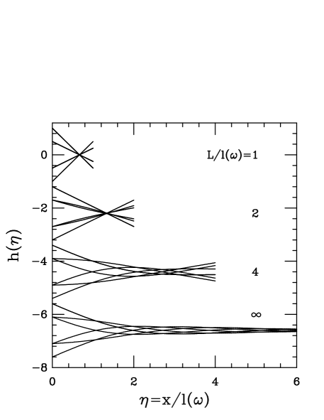
FIG. 8.: Solutions to EHD problem II for filaments of various rescaled lengths ${\cal L}$.

The solution consistent with the two left-end boundary conditions is

$$y= {y_{0}\over 2}\Bigl{[} {\rm e}^{-C_{8}\eta}\cos\left(S_{8}\eta+\omega t\right)$$ (74)

$$+ {\rm e}^{-S_{8}\eta}\cos\left(C_{8}\eta-\omega t\right)\Bigr{]},$$ (75)

where $C_{8}=\cos\left(\pi/8\right)$ and $S_{8}=\sin\left(\pi/8\right)$. Compare with the solution to SII, Eq. 64. The semiinfinite solution (75) is shown at the bottom of Fig. 8 for $\omega t=n2\pi/6$, $n=1\ldots 6$. In the hydrodynamic case, the solution 64 describes exponentially decaying right-moving traveling waves of transverse velocity. In the elastohydrodynamic case, the higher-order derivative allows more complicated behavior: right and left-moving waves of displacement, with different decay rates and velocities. In this case, the right-movers have a slower decay (since $S_{8}\simeq 0.38<0.92\simeq C_{8}$), and might be expected in some sense to dominate over the left-movers. This mechanism will be elaborated on in section V D.

C Finite polymer

In the limit of a short or stiff polymer, ${\cal L}\ll 1$, we may expand the coefficients $c_{j}\left({\cal L}\right)$ appearing in the exact solution to find

$$h_{\ll}\left(\eta\right) \simeq\left({z_{0}{\cal L}}/8\right) \left[\sin\left(z_{0}\eta\right)-\sinh\left(z_{0}\eta\right)\right]$$ (76)

$$+\left(1/2\right) \left[\cos\left(z_{0}\eta\right)+\cosh\left(z_{0}\eta\right)\right]$$ (77)

$$-\left(3/4z_{0}{\cal L}\right) \left[\sin\left(z_{0}\eta\right)+\sinh\left(z_{0}\eta\right)\right]~{}.$$ (78)

The apparently singular result $h\sim{\cal L}^{-1}$ is shown illusory by rewriting $\eta=\alpha{\cal L}$, $\alpha=x/L\in\left(0,1\right)$ and expanding (78) for small ${\cal L}$, yielding

$$h_{\ll}\left(\alpha\right) \simeq \left(1-{3\over 2}\alpha\right)$$ (80)

$$+{i\alpha{\cal L}^{4}\over 1680}\left(-16+70\alpha^{2}-70\alpha^{3}+21\alpha^{4}\right)~{}.$$

Equivalently, we may derive this polynomial by truncating a series expansion for $h$ in $\alpha$ and enforcing the equation of motion (69) and the boundary conditions (9).

Using $h_{\ll}\left(\eta\right)$ (in 78), the boundary conditions at $x=0$ and Eq. 69 are satisfied exactly, whereas the boundary conditions at $x=L$ are satisfied to order ${\cal O}\left({\cal L}^{5}\right)$. Using $h_{\ll}\left(\alpha\right)$ (in 80), all four boundary conditions are satisfied exactly, whereas Eq. 69 is solved to order ${\cal O}\left({\cal L}^{4}\right)$.

The exact solution is shown in Fig. 8 for ${\cal L}=1,2,4$, and $\infty$ and $\omega t=n2\pi/6$, $n=1\ldots 6$. Note the existence of a pivot point at $x={2L/3}$ as ${\cal L}\rightarrow 0$. This behavior is described by the ${\cal O}({\cal L}^{0})$ term in Eq. 80: as ${\cal L}\rightarrow 0$, the polymer acts as a rigid rod. As a consequence, it is impossible to tell if a movie of such a polymer is being played forward or backward. Indeed, this is a filamentous version of the famous “one-armed swimmer” or “scallop” example illustrating the lack of net propulsion for rigid objects executing time-reversible motions in low Reynolds number flow [28, 4].

D Propulsive force

Problem II and its associated experiment are sufficiently reminiscent of flagellar hydrodynamics to motivate a calculation of the propulsive force $F$ generated in the $x$ direction by the wiggling. This can be done by integrating ${\bf f}_{\cal E}$, the force exerted by the polymer on the fluid, along the length of the filament. We then contract this instantaneous total force with ${\bf{\hat{e}}_{x}}$ and average over one period. This force is equal and opposite the propulsive force exerted by the fluid on the polymer.

Noting that the force per unit length in Eq. 7 is a total derivative,

$${\bf f}_{\cal E}=A\partial_{s}\left(\kappa_{s}{{\bf{\hat{n}}}}-{1\over 2}\kappa^{2}{\bf{\hat{t}}}\right),$$ (81)

and recalling the boundary conditions imposed on $\kappa$ and $\kappa_{s}$, we have

$$F\equiv-\int ds~{}{\bf f}_{\cal E}\cdot{\bf{\hat{e}}_{x}} = -A{\bf{\hat{e}}_{x}}\cdot\left(\kappa_{s}{{\bf{\hat{n}}}}-{1\over 2}\kappa^{2}{\bf{\hat{t}}}\right)\biggl{|}_{0}^{L}$$ (82)

$$= A{\bf{\hat{e}}_{x}}\cdot\left(\kappa_{s}{{\bf{\hat{n}}}}\right)\left(s=0\right)$$ (83)

$$= A\kappa_{s}\sin\theta\left(s=0\right).$$ (84)

This is geometrically exact. We now wish to calculate the time average over one period, which we denote by $\langle\cdots\rangle$. Within the linearized solution, $\kappa_{s}\sin\theta\simeq y_{xxx}y_{x}$. Recalling the expression for $y$ in Eq. 68, and expressing the answer in terms of the rescaled variable $\eta$, we obtain

$$F = A\langle y_{x}y_{xxx}\rangle$$ (85)

$$= {Ay_{0}^{2}\over 2\ell(\omega)^{4}}\Re\left(h_{\eta}h_{\eta\eta\eta}^{*}\right)$$ (86)

$$= {y_{0}^{2}\zeta\omega\over 4\sqrt{2}}\Upsilon\left({L\over\ell(\omega)}\right)$$ (87)

where ^∗ indicates complex conjugation, $\ell(\omega)$ is the characteristic length, and $\Upsilon$ is a scaling function conveniently normalized (see below).

The exact solution to EHDII given in Appendix C can be used to calculate the function $\Upsilon$ for all values of the polymer length. The asymptotic behavior as ${\cal L}\rightarrow\infty$ is

$$\Upsilon({\cal L})\rightarrow 1+4{\rm e}^{-2S_{8}{\cal L}}\sin\left(2C_{8}{\cal L}\right).$$ (88)

When the length is short compared to the characteristic length, so the polymer flexes very little,

$$\Upsilon\simeq{11\over 3360}{\cal L}^{4}+{\cal O}\left({\cal L}^{8}\right)\simeq{11\over 3360}{\zeta\omega\over A}L^{4}.$$ (89)

As Fig. 9 illustrates, the short-length approximation (89) shows good agreement with the exact solution for ${\cal L}\lesssim 3$, as does the large-${\cal L}$ approximation (88) for ${\cal L}\gtrsim 3$. The approach to the asymptotic limit is oscillatory, with a maximum near ${\cal L}\sim 4$, the value at which $\Re\{h_{\eta}\}$ acquires its first root, and a local minimum near ${\cal L}\sim 6$, the the value at which $\Im\{h_{\eta}\}$ acquires its second root. The unexpected local maximum indicates that there is an optimal combination of $A,\omega$, and a finite $L$.

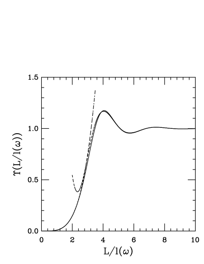
FIG. 9.: Scaling function $\Upsilon$ for propulsive force. The large ${\cal L}$ expansion is plotted for ${\cal L}>2$, and the small-${\cal L}$ solution is plotted for ${\cal L}<3.5$.

Inserting typical numbers from the experiment (in cgs),

$$\mu\sim 10^{-2},~{}y_{0}~{} \sim 4\times 10^{-4}$$ (90)

$$\omega\sim 2\pi,~{}{L\over d} \sim{7\times 10^{-4}\over 7\times 10^{-7}}=10^{3}$$ (91)

we find ${F(\infty)}\sim 2\times 10^{-9}$ dynes $=3\times 10^{-2}$ pN. For a trap stiffness of $\sim.02$ pN/nm, this would induce a displacement of $1.5$ nm, at the lower limit of experimental observation. The production and measurement of propulsive force by an artificial flagellum was attempted by G. I. Taylor [32] using a glycerine-filled tub to mimic the low Reynolds numbers found in vivo. Taylor struggled to drive the flagellum without inducing unwanted torque or disturbing the flow, a difficulty obviated by the use of optical traps.

Returning to the asymptotic expressions for $h$ derived in the sections V B and V C, we observe a pleasant accordance with the qualitative features of Fig. 9. In the semiinfinite case, we noted the presence of right- and left- movers, with right-moving waves of displacement exhibiting slower decay. Such a dominance accounts for the nonzero propulsive force in the ${\cal L}\rightarrow\infty$ limit, where a net propulsion to the left survives. In the ${\cal L}\rightarrow 0$ case, we recovered a shape which asymptotes to a pivoting rigid rod, not unlike a one-armed swimmer. As we expect from life at low Reynolds number [28, 4], such a motion, invariant under $t\rightarrow-t$, can produce no net propulsion.

As further illustration of the relationship between low-Reynolds-number swimming and cyclic motions, we observe that the lowest-order expression for the time-averaged force is equal to

$$F={\zeta\omega\over 2\pi}\int_{0}^{2\pi/\omega}dt~{}y_{x}|_{x=0}\partial_{t}\int_{0}^{L}dx~{}y(x)$$ (92)

or, noting that $\int dx~{}y(x,t)$ is simply the area ${\mathcal{A}}(t)$ under the curve $y(x,t)$, and that the slope at the left is to first order simply the tangent angle $\theta_{0}$

$$F = {\zeta\omega\over 2\pi}\int_{0}^{2\pi/\omega}dt~{}\theta_{0}~{}{d{\mathcal{A}}\over dt}$$ (93)

$$= {\zeta\omega\over 2\pi}\oint\theta_{0}d{\mathcal{A}}.$$ (94)

This result can be interpreted quite simply: the propulsive force results from pushing aside some volume (or in two dimensions an area) of fluid, projected in the direction of propulsion ${\bf{\hat{e}}_{x}}$ an amount proportional to $\theta_{0}$. Note that had we been interested in the propulsion in the transverse (${\bf{\hat{e}}_{y}}$) direction, the $\theta_{0}$ would not appear, leaving the absence of net forcing: $F\propto\oint d{\mathcal{A}}=0$, as we would expect.

The net force, then, is the area enclosed by a trajectory in ${\mathcal{A}}-\theta_{0}$ space during some cyclic motion. This representation is independent of the particular motion exhibited, although we have here considered simple periodic motion, for which the trajectory is always an ellipse. As ${\cal L}\rightarrow 0$, the elliptical trajectory thins to a straight line, encloses no area, and thus produces no force, as commented on above.

This representation makes clear that in an inertialess world, net motion is principally geometric in origin rather than dynamic.[36] In a manner analogous to the importance of path rather than kinetics in generating net work in a Carnot diagram, we see that we can remove time entirely from the expression and consider instead a path in a low-dimensional projection of the infinite-dimensional shape space.

VI Experiments on actin

As mentioned in section V, the EHDII experiment was performed and the data compared to the solution of Eq. 69. In this way we were able to confirm the results of the analysis and investigate a new method for measuring biopolymer bending moduli.

A Materials and methods

Actin from white leghorn chicken breast was purified after a published procedure[27]. Filamentous actin (F-actin) was fluorescently labeled with rhodamine-phalloidin (R-415, Molecular Probes, Inc.). Anti-actin antibodies (Sigma) were covalently coupled through carbodiimide to fluorescent polystyrene beads (CX, Duke Scientific Corporation), of diameter 1 mm, after the recommended protocol of Duke. Experiments were performed in actin suspension buffer containing 25 mM imidazole, 25 mM KCl, 5 mM b-mercaptoethanol at pH 7.65. To avoid photobleaching during observation, 1mg/ml glucose, 33 units/ml glucose oxidase, 50 units/ml catalase were added to the suspension buffer.

In order to prevent actin filaments from sticking to the glass surfaces, slides were coated with bovine serum albumin (BSA). Observation chambers were sealed with nail polish and filled by capillary action. Beads and F-actin coupled within the cell; the ratio beads:F-actin was adjusted to have one or two beads per filament. Beads bound to various locations along filaments. Among these filaments, we chose bead-ended actin filaments for the experiment.

Observations were made on a Zeiss microscope (Axiovert 135) equipped with a 100 W mercury lamp and a standard filter set (XF37, Omega optical). To prolong observation time, the excitation light intensity was reduced by inserting neutral density filters. Fluorescent images were taken through a 4X TV tube, via an image intensifier (Hamamatsu) followed by a CCD camera (XC-77, Sony). Images were recorded with an S-VHS recorder. Images corresponded to an overall screen size of 44 mm in horizontal dimension leading to a value of 0.06mm/pixel after digitization. Fig. 7 shows the experimental setup, and Fig. 10 shows a series of typical images. The smooth curves indicate fit solutions to Eq. 69.

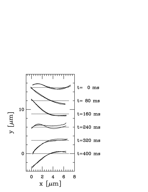
FIG. 10.: Series of typical images of driven actin filaments in EHDII. Also shown are fits to the solution of Eq. 69.

The optical tweezer was made by focusing a 0.5 W Nd:YAG (Spectra) laser beam through a Zeiss 63X, 1.4 numerical aperture Plan-Apochromat microscope objective. A mirror mounted on a galvanometer controlled by a function generator served to move trapped beads in the focal plane (Fig. 7). We imposed sinusoidal driving, with frequencies and amplitudes ranging, respectively, from 0.1 Hz to 6 Hz and from 5 $\mu$m to 10 $\mu$m.

Up to 10 images per oscillation period were digitized with a Scion frame grabber card and a Power Macintosh; they were subsequently analyzed using NIH-Image software. Each image was retraced by mouse and its coordinates determined. Only those sequences for which filaments remained in the focal plane for an oscillation period were retained for data analysis.

B Experimental results

Knowing the amplitude of the driving of the bead ($y_{0}$) and the frequency ($\omega$), and reading off the projected length ($L$) and the phase ($\omega t$) directly from the images, we were left with a one-parameter fit of the images to the solution of Eq. 69, varying only $\ell(\omega)$ to minimize $\chi^{2}$. We can then observe the dependence of $\ell$ on $\omega$, as illustrated in Fig. 11. The variation in error bars can be attributed to the widely-varying numer of images taken at different frequencies.

Comparing with the earlier analysis (cf.  section V A), we can extract from this scaling a measurement of the persistence length. Fitting to

$$\ell(\omega)={\left(k_{B}T\over\zeta\right)}^{1/4}L_{p}^{1/4}\omega^{-1/4},$$ (95)

we determine $L_{p}$ to be $7.37\pm 0.25\mu m$.

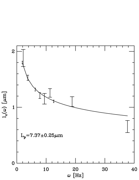
FIG. 11.: The characteristic length scale $\ell(\omega)$ vs. frequency $\omega$. The smooth curve is a fit to Eq. 95 for $L_{p}=7.37\mu$m. The scaling of the characteristic length with the fourth root of time suggests that actin is well-described by Eq. 2 and thus is a semiflexible polymer, with a scale-independent elasticity.

C Discussion

There are a few limitations with this realization of the experiment which, upon correction, will improve this technique and make the data more conclusive. An obvious mechanism for improving the error bars is to accumulate more data. Image-taking was entirely manual, with hundreds of student-hours spent looking for usable images. An automation of this process would clearly be advantageous and improve the low statistics used here.

With careful control of the timing, images of equal phase can be superposed to average out thermal fluctuations or experimental variation in the images before fits are performed.

Most importantly, since our aim was to verify the plausibility of the experiment, we did not limit ourselves to small-amplitude wiggling, thus leaving the realm of validity of the small-$y_{x}$ approximation. We can estimate the error due to such driving by looking at the relevant terms from the geometrically exact equation of motion:

$${y_{t}\over{({1+y_{x}^{2}})^{1/2}}}=-{\tilde{\nu}}\left({y_{xx}\over{\left(1+y_{x}^{2}\right)^{3/2}}}\right)_{ss},$$ (96)

If we wish to approximate this with Eq. 10, we are measuring an “effective” ${\tilde{\nu}}$, or ${``{{\tilde{\nu}}}"}$, where

$${``{{\tilde{\nu}}}"}\simeq{{\tilde{\nu}}\over\langle\left(1+y_{x}^{2}\right)^{2}\rangle},$$ (97)

where the brackets indicate averaging over the data, and thus the true $A$ will be underestimated by a factor of $\langle({{1+y_{x}^{2}}})^{2}\rangle$, which is always greater than unity. Inspecting Fig. 10, we see that there are data for which $y_{x}$ is not necessarily small. For this reason, the data we collected can only put a lower bound on $A$. We anticipate that the true value may be greater by a factor up to $\sim 1.5$; future experiments clearly should employ smaller-amplitude driving.

D Suggestions for further analysis

We also anticipate that a more accurate treatment of the geometry and hydrodynamics would refine the technique. The true geometry is nonlinear and hydrodynamics nonlocal, but neither intractable and both amenable to numerics. The geometrically exact, intrinsic formulation involves some enjoyable mathematics of curve dynamics, [3] whereas the linearized treatment presented herein is more illustrative and more easily connected with experiment. Similarly, in an attempt to make the analysis as clear as possible, we have omitted from Eq. 10 the background flow due to the trapped bead.

Some amount of discussion has been entertained in the biophysical community about the possible scale- or time-dependence of the elasticity of biopolymers, including both actin [16] and microtubules [18]. One of the more powerful features of this technique is that, since it involves a controlled dynamic, specific scales and frequencies can be investigated to attempt a spectroscopy of elasticity. Equation 10 can be extended without difficulty to include a characteristic relaxation time $\tau$ or a continuum of times, in an attempt to model a characteristic rate of bond-breaking in the presence of bending. Similarly, one can include additional bending moduli which depend on higher-order derivatives. For oscillatory motion, occurrences of $\partial_{t}$ are simply replaced by $\partial_{t}+{1/\tau}$ or ${i\omega+1/\tau}$. Including higher-order derivative terms simply results in replacing $Ay_{2x}$ with $Ay_{2x}+By_{4x}$ in the bending energy and $Ay_{4x}$ with $Ay_{4x}+By_{8x}$ in the equations of motion. We then may recover such an equation as

$$\zeta(\partial_{t}+{1\over\tau})y=-Ay_{xxxx}-By_{8x},$$ (98)

which may be solved in the manner of Eq. 2. This more general expression makes possible the experimental confirmation or refutation of such hypothesized mechanisms.

VII Comments on previous experiments

A recent pair of elastohydrodynamic experiments involving microtubules [10], brought to our attention as the original version of this paper was being completed, provides an excellent opportunity to apply the spirit of analysis which we have developed for EHDI. In both, the crucial experimental observable is the motion of the free end of a microtubule; the analysis must then relate this motion to the bending modulus $A$. We will first investigate the analysis appropriate to a special case of EHDI in which a polymer relaxes to a straight configuration in the absence of a driving flow. We then investigate a more complicated experiment in which an optical trap induces a force in the middle of the polymer.

A The Simple EHDI experiment

In the first experiment [10], a microtubule is initially clamped at the left to an axoneme and trapped directly at the free end; the polymer is bent out of its mechanical equilibrium configuration. When the trap is shut off, the polymer relaxes back to the straight shape in a way which we may describe as before: the initial condition is projected onto the appropriate space, in which each mode decays independently.

FIG. 12.: EHDI experiments. (a) a simple special case (b) end-driving as well as driving via a point force.

What remains then is merely to determine the initial data: the shape of a biopolymer clamped at one end and held by a trap at the other. We may derive this from the (geometrically exact) general equations of force and torque balance for the elastica:

$${\bf N}_{s}+{\bf f}_{e}=0$$ (99)

$${\bf m}_{s}+\left({\bf r}\times{\bf N}\right)_{s}+{\bf r}\times{\bf f}_{e}=0$$ (100)

Here ${\bf N}$ is a contact force (not the unit normal), ${\bf m}$ is a bending moment, and ${\bf f}_{e}$ is some external force. While these equations may appear unfamiliar, they in fact have a long history as the classical forms of the equations of equilibrium for the special theory of Cosserat rods [2]. Combining the equations into one,

$${\bf m}_{s}={\bf{\hat{t}}}\times\int_{0}^{s}d\sigma~{}{\bf f}_{e}\left(\sigma\right)~{},$$ (101)

where ${\bf{\hat{t}}}={\bf r}_{s}$ is the unit tangent. In two dimensions, cross products are scalars, and ${\bf m}_{s}$ becomes the scalar $m_{s}$.

We now include the defining constitutive relation of linear elasticity: $m=A\theta_{s}$. Furthermore, in considering point external forces (the axoneme and the trap) that act at the left and right ends, we write

$${\bf f}_{e}(s)={\bf F}_{0}\delta(s)+{\bf F}_{1}\delta(s-L)~{}.$$ (102)

We assume that there is no net force, so ${\bf F}_{0}=-{\bf F}_{1}$. Noting that ${\bf{\hat{t}}}=\left(\cos\theta,\sin\theta\right)$ we rewrite Eq. 101 (for $0<s<L$) as

$$A\theta_{ss}=-F_{y}\cos\theta+F_{x}\sin\theta$$ (103)

where $F_{\{x,y\}}$ are the components of the force exerted by the trap, rather than by the axoneme. We expect $F_{x}<0$ and $F_{y}>0$. Eq. 102 is geometrically exact and can be solved in terms of elliptic integrals.

Note that there is no reason to assume the trap exerts a force only in the ${\bf{\hat{e}}_{y}}$ direction – the oft-quoted “cantilevered beam” problem from introductory civil engineering texts. We show below, however, that the ${\bf{\hat{e}}_{x}}$ component is higher order in $\theta$ and will be ignored in the linearized treatment presented. Linearizing Eq. 103 for small $\theta$ obtains

$$A\theta_{ss}=-F_{y}+\theta F_{x},$$ (104)

the windy pendulum equation[35]. Assuming the polymer is homogeneous along its arclength, we note that there is no energy cost upon moving the trap along the axis of the polymer. Therefore the trap can exert no force in the tangential direction. We may write this constraint

$$0={\bf F}\cdot{\bf{{\bf{\hat{t}}}}}\simeq F_{x}+F_{y}{dy\over dx}~{}.$$ (105)

Accordingly, $F_{x}/F_{y}\simeq-dy/dx$, and Eq. 104 becomes

$$Ay_{xxx}\simeq-F_{y}\left(1+{\cal O}(y_{x}^{2})\right)~{}.$$ (106)

We now must consider the boundary conditions. The axoneme clamps the left end of the polymer, thus $\nobreak{y\left(0\right)=y_{x}\left(0\right)=0}$. Since there is no energy cost to rotating a polymer held in an optical trap, there should be no bending moment, implying $y_{xx}\left(L\right)=0$. Given these three boundary conditions, the solution to (106) is

$$y\left(x\right)={{\tilde{y}}\over 2}\left(3\alpha^{2}-\alpha^{3}\right)~{},\ \ \ \ {\tilde{y}}=y(L)={F_{y}L^{3}\over 3A}~{},$$ (107)

where again $\alpha\equiv x/L$.

Now that we have our initial data, we project it onto the appropriate function space in which the dynamics are simply exponential relaxation. In keeping with the experiment we seek here to model, we focus on the motion of the free end, whose rate of relaxation provides a direct means of measuring the bending modulus $A$. Given the dramatic increase in relaxation rates for each subsequent mode (cf.  Eq. 32), we expect only the lowest mode to be relevant beyond negligible initial times. Moreover, inspecting Fig. 6, we observe that the eigenfunction ${\cal W}_{k_{1}}$ well-approximates the normalized third-order polynomial which describes the initial data, whereas higher modes more closely resemble Fourier modes. This close agreement, rather surprising from a sum of trigonometric and hyperbolic trigonometric functions, leads to the dominance of the projection of initial data onto the first mode; specifically

$$y_{k_{1}}\left(0\right)\simeq 0.971~{}{\tilde{y}};~{}~{}~{}y_{k_{2}}\left(0\right)\simeq-0.0247~{}{\tilde{y}}~{},$$ (108)

where we define $y_{k_{n}}\equiv\int_{0}^{1}d\alpha~{}y{\cal W}_{k_{n}}$, in analogy to Eq. 32. Inserting typical numbers ($A\sim 5\times 10^{-15}$ dynes cm², $L\sim 10\times 10\mu$m, and the drag coefficient from Eq. 12 with $d\sim 20$nm and $\mu\sim.01$ erg s/cm³), we see that for times beyond $0.01$s, the amplitudes of subsequent modes are at most 1% that of the first mode. The shape is then described by $y\left(x\right)\simeq{\cal W}_{k_{1}}\left(x\right)y_{k_{1}}\left(t\right)$ and decays as ${\rm e}^{-rt}$, with $r\equiv{Ak_{1}^{4}/\zeta L^{4}}$. In the model accompanying the experiment, it was assumed that the shape was described by a single decaying mode for all times up to $t=0$. As we have shown, ${\cal W}_{k_{1}}$ fortunately well-approximates the initial data such that this introduces only an error ${\cal O}(10^{-2})$.

Within these approximations, the free end decays as

$${y\left(L,t\right)\over y\left(L,0\right)}\simeq 0.971{\cal W}_{k_{1}}\left(L\right){\rm e}^{-rt}\simeq{\rm e}^{-rt}.$$ (109)

so that a measurement of the e-folding time yields $r$ and hence $A$. It is now clear that the identity of $k_{1}$, the solution to the transcendental equation (36), is crucial, as it is physically manifested in the decay rate.

The model in [10] is based first on the computation of the deflection $y_{l}$ of the free end of the clamped elastica experiencing a flow linearly increasing in $x$ and constant in time, with a drag coefficient $\tilde{\zeta}$. Such a flow would be appropriate for a rigidly rotating rod with constant angular velocity, rather than for a bent filament. Second, to find the decay rate in [10], it is noted that the exponential relaxation of the tip must correspond to some first-order differential equation. Although this equation is not stated, we must assume it to be $y_{t}(t)=-(v/y_{l})y(t)$, (where $v$ is the maximum flow velocity used in the computation of $y_{l}$) in order to recover the reported decay rate,

$$r={120\over 11}{{``A"}\over\tilde{\zeta}L^{4}}.$$ (110)

where ${``A"}$ refers to the value of $A$ which would be extracted from data, using the simplifications described above.

A careful analysis of the drag coefficient in slender-body hydrodynamics employs a matched asymptotics for the fluid velocity and is dependent on the shape of the slender body. Treating a microtubule as a cylinder, the appropriate drag coefficient is [6]

$$\zeta={4\pi\mu\over\ln\left(L/d\right)+2\ln 2-{1\over 2}}.$$ (111)

Unfortunately, the drag coefficient used in [10] is that appropriate to tangential rather than normal flow, with numerator $2\pi\mu$ (quoting an earlier misquotation of Doi and Edwards[33, 9]) and further suffers from the replacement of the constant terms in the denominator of Eq. 111 with $-\ln 2$.

We may now compare the results of a differential equation-motivated analysis with the model of [10]. Given some measured e-folding time $t_{*}$, the eigenmode analysis yields the bending modulus $A$ as

$${A}={\zeta L^{4}\over t_{*}}k_{1}^{-4}$$ (112)

whereas the rodlike treatment implies (from Eq. 110)

$${``A"}={\tilde{\zeta}L^{4}\over t_{*}}{11\over 120}.$$ (113)

Inserting typical numbers from the experiment, $L\sim 10\mu{\rm m}$, $d\sim.02\mu{\rm m}$, we see that

$${{``A"}\over{A}}=1.13{\tilde{\zeta}\over\zeta}\simeq 0.709,$$ (114)

a systematic underestimate beyond the uncertainties of experiments.

B The discontinuous EHDI experiment

A more complicated example of EHDI which was also conducted includes driving the axoneme, so that we must incorporate an inhomogeneous boundary condition, and point forcing by an optical trap [10]. In this experiment, the axoneme (attached to the cover slip) is moved with constant velocity between two extreme positions. During this motion, the polymer is constrained by the optical trap to pass through some intermediate point $(x_{p},y_{p})$. From the position and velocity of the free end it is possible to determine the bending modulus. Enumerating all the relevant forces, we consider the force at the left end due to the axoneme, $F_{a}$, the point force due to the trap $F_{p}$, and the force per unit length due to drag, $-\zeta h_{t}$ (cf.  Fig. 12). We insert these terms into the equations of force and torque balance (99,100) to find the equations of motion.

1 Explicit declaration of forces

The sum of the external forces per unit length can be expressed as

$${\bf f}_{e}:={\bf F}_{p}\delta\left(s-s_{p}\right)+{\bf F}_{a}\delta\left(s\right)+{\bf f}_{d}$$ (115)

where ${\bf f}_{d}$ is the drag (Eq. 10).

Integrating over the delta functions, and taking the axoneme to be located at $s=0$, the geometrically exact governing equation (101) becomes the fiercely complicated integro-differential equation in $\theta(s,t)$

$$A\theta_{ss} = {\bf{\hat{t}}}\times\biggl{[}{\bf F}_{a}+{\bf F}_{p}\Theta\left(s-s_{p}\right)$$ (117)

$$\qquad+\zeta\int_{0}^{s}\!d\sigma\left({\bf{\hat{n}}}{\bf{\hat{n}}}+\beta{\bf{\hat{t}}}{\bf{\hat{t}}}\right)\left(\int_{0}^{\sigma}\!d\sigma^{\prime}{\bf{\hat{n}}}\theta_{t}-{\bf u}\right)\biggr{]},$$

which greatly simplifies for small $y_{x}$. Here $\bf u$ is the background flow velocity, in the frame of the trap, due to the motion of the coverslip. This is a constant for the problem, which we define to be $-v_{c}{\bf{\hat{e}}_{y}}$ so that $v_{c}>0$. Note that the axoneme, attached to the coverslip, also moves with velocity $-v_{c}{\bf{\hat{e}}_{y}}$. We see that point forcing in the middle of a polymer introduces a qualitative change in the dynamic: a Heaviside function in the equation of motion.

2 Linearized geometry

We adopt an expansion in $\theta$, keeping only the first-order terms. The drag term, as in Eq. 14, simplifies to $\zeta{\hat{\bf e}}_{y}(y_{t}+v_{c}).$

Noting, as in Eq. 105, the constraint that the force on a polymer due to an optical trap must have no tangential component, the $y$-component of the linearized equation reduces to $A\theta_{ss}\simeq F_{a}-F_{p}\Theta\left(s-s_{p}\right)-\zeta(\int^{s}y_{t}+v_{c}),$ which upon differentiation and linearization implies

$$\zeta(y_{t}+v_{c})=-Ay_{xxxx}-F_{p}\delta\left(x-x_{p}\right).$$ (118)

This is our working equation, obtained from the linearized second derivative of the equation of net torquelessness.

Since we do not know the magnitude of $F_{p}$ a priori, we must perform a matching of $y^{a}\left(x\right)$, the curve described by the anchored end, and $y^{f}\left(x\right)$, the curve described by the free end, which solve

$$\zeta(y_{t}^{\{a,f\}}+v_{c})=-Ay_{xxxx}^{\{a,f\}}$$ (119)

subject to matching conditions at the point of forcing. Horrifying though this may sound, it is an excellent opportunity to apply the simple ideas developed in earlier sections. It is also, of course, a chance to treat in a thorough way the analysis of a biopolymer subject both to drag and to micromanipulation via some point force and boundary condition. Moreover, if we wish to claim that the PDE description is the appropriate analysis for single biopolymer dynamics, we must be able to apply it even to such an awkward case. We will separate the solutions into the homogeneous and the particular, and in a procedure that is now familiar, construct the appropriate function space in which the dynamic is simple.

3 Matching and boundary conditions

Now that we have two fourth-order equations of motion, we must specify eight matching and boundary conditions. Inspecting the equation of motion (Eq. 118), we see it supports a discontinuity in $y_{xxx}$; however, $y_{xx}$, described by an integral over a Heaviside function, is continuous, as are $y$ and $y_{x}$. Moreover, if we wish to describe an experiment in which the filament position is constrained at the point of forcing $x_{p}$, we have not only the matching condition $y^{a}(x_{p})=y^{f}(x_{p})$, but the stronger condition $y^{a}(x_{p})=y^{f}(x_{p})=y_{p}$; here we choose $y_{p}$ to be $0$ without loss of generality. We are thus describing a polymer pinned at a certain intermediate point along the curve by an optical trap, while the right and left sides perform some coupled motion.

At the free end, we impose forcelessness and torquelessness, stated linearly as $y_{xxx}\left(L\right)=0$ and $y_{xx}\left(L\right)=0,$ respectively. At the anchored end, we describe a polymer clamped to the axoneme position $y_{A}(t)$, thus $y\left(0\right)=y_{A}(t);~{}~{}y_{x}\left(0\right)=0.$ The above-listed boundary conditions constrain $4$ of the arbitrary constants, the remaining matching equations constitute the remaining $4$, and we may thus completely specify the solution.

4 Construction of the inhomogeneous solution

The governing equation is linear, allowing us to separate $y$ into two separate solutions of Eq. 119: $y=y_{0}(h+g)$, where $y_{0}$ is some typical length scale. We choose $g$ ($h$) to satisfy the (in)homogeneous boundary conditions and equation of motion. Compare this with the first example solution of EHDI (section IV B), in which $h$ was chosen to satisfy an inhomogeneous equation of motion but homogeneous boundary conditions.

As described above, the axoneme moves with constant velocity $v_{c}$ from $y_{A}=\Delta$ to $y_{A}=-\Delta$: $y_{A}\left(t\right)=-v_{c}t,\ \ (-{\Delta/v_{c}}<t<{\Delta/v_{c}}).$ We must now merely solve for the inhomogeneous solution, expressed as

$$h^{\{a,f\}}\left(x,t\right)\equiv\sum_{n=0}^{\infty}c_{n}^{\{a,f\}}\left(t\right)x^{n}.$$ (120)

However, as in the derivation of Eq. 46, we expect this solution to depend only linearly on the driving and thus linearly on time. Constraining $\partial_{t}^{2}c^{\{a,f\}}_{n}=0,$ enforcing the 8 matching and boundary conditions, and respecting the relationship between $\partial_{t}c_{n}$ and $c_{n+4}$ dictated by Eq. 119, we completely specify the solution.

5 Polynomial solution

We here quote the solutions for $h^{\{a,f\}}$. In order to make explicit the qualitative behavior in limiting cases, and to write the solutions as compactly as possible, we employ three nondimensionalized variables:

$$\alpha\equiv{x\over x_{p}},~{}~{}\sigma\equiv{{x-x_{p}}\over{L-x_{p}}}~{},~{}~{}\tau\equiv t{A\over\zeta x_{p}^{4}}.$$ (121)

The coordinates $\{\alpha,\sigma\}\in(0,1)$ measure distance on the left from the axoneme and on the right from the trap, while $\tau$ is the time rescaled by the characteristic elastohydrodynamic time for the anchored section. The fact that $x_{p}$, rather than $l\equiv L-x_{p}$, appears explicitly in our choice of definition of $\tau$ is reflected in the equation of motion, in that the functions now solve slightly different equations for the two sides:

$$h_{\tau}^{a}+{v_{c}\over y_{0}}{\zeta x_{p}^{4}\over A} = -h^{a}_{\alpha\alpha\alpha\alpha};$$ (122)

$$h_{\tau}^{f}+{v_{c}\over y_{0}}{\zeta x_{p}^{4}\over A} = -\left({x_{p}\over l}\right)^{4}h^{f}_{\sigma\sigma\sigma\sigma}.$$ (123)

The natural choice for $y_{0}$ is clearly $y_{0}=v_{c}\zeta x_{p}^{4}/A$, whereupon we are left with the dimensionless equations of motion

$$h_{\tau}^{a}+1 =- h^{a}_{\alpha\alpha\alpha\alpha};~{}~{}$$ (124)

$$h_{\tau}^{f}+1 =- \rho^{4}h^{f}_{\sigma\sigma\sigma\sigma}~{},$$ (125)

where we have introduced the ratio of lengths

$$\rho\equiv{x_{p}\over{L-x_{p}}}={x_{p}\over l},~{}~{}$$ (126)

which describes the location of the point of forcing $x_{p}$ relative to the “extra” length $l$. As $x_{p}$ nears the anchored end $x=0$, $\rho\rightarrow 0$, and as $x_{p}$ nears the free end $x=L$, $x_{p}/(L-x_{p})=\rho\rightarrow\infty$.

The expressions are then:

$$h^{f}\rho^{5} = -{\frac{1}{80}}\sigma^{5}-{\frac{1}{24}}\rho\sigma^{4}+\left({\frac{\rho}{6}}+{1\over 8}\right){\sigma}^{3}-\frac{1}{4}\left(\rho+1\right){\sigma}^{2}$$ (128)

$$+\left({\frac{1}{105}}\rho^{4}-{\frac{1}{8}}\rho^{2}-{\frac{1}{8}}\rho+{\frac{3}{2}}\rho^{4}\tau\right)\sigma$$

$$h^{a}\rho^{3} = {\frac{1}{1680}}{\alpha}^{7}{\rho}^{3}-{\frac{1}{240}}{\alpha}^{6}{\rho}^{3}-{\it\tau}\,{\rho}^{3}$$ (131)

$$+\left({\frac{13}{560}}\rho^{3}-{\frac{1}{8}}\rho-{1\over 8}-{\frac{1}{2}}\rho^{3}\tau\right){\alpha}^{3}$$

$$+\left(-{\frac{11}{560}}\rho^{3}+{\frac{1}{8}}\rho+{1\over 8}+{\frac{3}{2}}\rho^{3}\tau\right){\alpha}^{2}.$$

6 Decaying modes

As described before, the solution $h$ to the inhomogeneous boundary conditions will describe the long-time behavior remaining as transients decay exponentially. We now turn our attention to the transient $g$, which must satisfy the following homogeneous boundary and matching conditions:

$$g(0)=0,~{}~{}g_{x}(0)=0,$$ (132)

$$g_{xx}(L)=0,~{}~{}g_{xxx}(L)=0$$ (133)

$$g\left(x_{p}\right)=0,~{}~{}[g_{x}\left(x_{p}\right)]=0,~{}~{}[g_{xx}\left(x_{p}\right)]=0,$$ (134)

where the brackets indicate discontinuity.

The fact that all the boundary conditions are $0$-valued means we stand a chance of constructing a self-adjoint operator, consistent with these conditions, from the relevant differential operator: $\partial_{x}^{4}$. To do so, we left-multiply the equation of motion by an as-yet arbitrary function ${\cal W}_{k}\left(x\right)$ and integrate over the entire domain. Since $h$ is constructed to solve the (linear) equation of motion (118), $g$ must as well, and we derive an equation of motion for the quantities $g_{k}\equiv\int_{0}^{L}dx{\cal W}_{k}(x)g(x)$:

$${1\over{\tilde{\nu}}}\partial_{t}g_{k}=-\int_{0}^{L}\!dx{\cal W}_{k}\left(x\right)g_{xxxx}{}~{}.$$ (135)

We then wish to integrate the RHS by parts. However, we must admit the possibility that $g$ supports a discontinuity in its higher-order derivatives, i.e.,  $[g_{xxx}\left(x_{p}\right)]\neq 0$. For this reason, we define $\{g^{a}\left(x,t\right),{\cal W}_{k}^{a}\left(x\right)\}$ and $\{g^{f}\left(x,t\right),{\cal W}_{k}^{f}\left(x\right)\}$, as in Eq. 119, defined on the anchored and free sections, respectively. If we choose ${\cal W}$ to obey the same homogeneous boundary conditions as $g$, all surface terms from the integration by parts in Eq. 135 vanish except

$$-\partial_{x}{\cal W}_{k}^{a}\partial_{x}^{2}g^{a}\left(x_{p}\right) +\partial_{x}{\cal W}_{k}^{f}\partial_{x}^{2}g^{f}\left({x_{p}}\right)$$ (136)

$$+\partial_{x}^{2}{\cal W}_{k}^{a}\partial_{x}g^{a}\left({x_{p}}\right) -\partial_{x}^{2}{\cal W}_{k}^{f}\partial_{x}g^{f}\left({x_{p}}\right)$$ (137)

which vanish upon choosing ${\cal W}$ to obey the same matching conditions as $g$. The remaining equation is

$$-{1\over{\tilde{\nu}}}\partial_{t}g_{k}=\int_{0}^{x_{p}}g^{a}\partial_{x}^{4}{\cal W}_{k}^{a}+\int_{x_{p}}^{L}g^{f}\partial_{x}^{4}{\cal W}_{k}^{f}.$$ (138)

We now choose ${\cal W}_{k}^{\{a,f\}}$ to obey the eigenvalue condition $\partial_{x}^{4}{\cal W}_{k}^{\{a,f\}}=k^{4}{\cal W}_{k}^{\{a,f\}}$. Since we have constructed a self-adjoint operator, we can be sure the eigenvalues are real and positive (cf. Appendix B). We are left with

$$-\partial_{t}g_{k} = {\tilde{\nu}}k^{4}\bigl{\{}\int_{0}^{x_{p}}{\cal W}_{k}^{a}g^{a}(x,t)+\int_{x_{p}}^{L}{\cal W}_{k}^{f}g^{f}(x,t)\bigr{\}}$$ (139)

$$= {\tilde{\nu}}k^{4}g_{k},$$ (140)

the solution of which is, as before, $g_{k}\left(t\right)=g_{k}\left(0\right){\rm e}^{-{\tilde{\nu}}k^{4}t}$ for $k\neq 0$. Fortunately, the boundary and matching conditions do not admit a solution to $g_{xxxx}=0$, and we need not consider a $0$ mode.

Given some initial condition $y(x,0)$, we project it onto this strange eigenspace spanned by $\{{\cal W}_{k}\}$. We then construct $g\left(x,t\right)$ for all later times in a standard Green’s function way,

$$g\left(x,t\right)=\int_{0}^{L}\!\!{dx^{\prime}\over L}{\cal G}\left(x,x^{\prime};t\right)\bigl{\{}{y\left(x^{\prime},0\right)\over y_{0}}-h\left(x^{\prime},0\right)\bigr{\}}$$ (141)

where

$${\cal G}=\sum_{k}{\rm e}^{-{\tilde{\nu}}k^{4}t}{\cal W}_{k}\left(x\right){\cal W}_{k}\left(x^{\prime}\right),$$ (142)

and we see that all modes die.

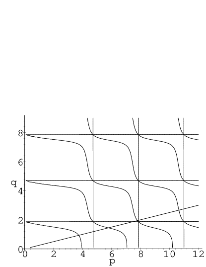
FIG. 13.: $p-q$ plane showing roots of the solvability condition. Here $p\equiv kx_{p}$ and $q\equiv kl=k(L-x_{p})$. The geometry of the experiment dictates $\rho$, as described in the text. Vertical and horizontal lines correspond to solutions of $F(p)=0$ and $H(q)=0$, respectively. The diagonal line indicates the solution to $x_{p}/L=.8$.

7 Construction of ${\cal W}_{k}$; solvability condition

We now solve for the countably infinite sets $\{k\}$ and $\{{\cal W}_{k}\}$. The general solution of $\partial_{x}^{4}{\cal W}_{k}^{\{a,f\}}=k^{4}{\cal W}_{k}^{\{a,f\}}$ is

$${\cal W}_{k}^{\{a,f\}}= a_{1}^{\{a,f\}}\sin\left(kx\right)+ a_{2}^{\{a,f\}}\cos\left(kx\right)$$ (143)

$$+ a_{3}^{\{a,f\}}\sinh\left(kx\right)+ a_{4}^{\{a,f\}}\cosh\left(kx\right),$$ (144)

where the $8$ arbitrary constants will solve the $4$ boundary and $4$ matching conditions. The insertion and elimination of these constants is not a joyful task and will be omitted here. The most important fact is that the set of $8$ equations for $8$ unknowns can be written as a matrix of trigonometric functions (as in Eq. 35) annihilating the vector ${\bf a}$ of unknowns. The $0$-valuedness of the conditions dictates that the determinant ${\cal D}$ of this matrix be $0$. This solvability condition is written explicitly in appendix D; the solutions, graphically constructed in Fig. 13, determine the allowed values of $k$ given some fixed ratio $\rho$.

Curiously, the complicated solvability condition can be expressed compactly as the separable equation

$${\cal D}=\partial_{p}F\left(p\right)H\left(q\right)+F\left(p\right)\partial_{q}H\left(q\right)=0,$$ (145)

where $F(p)\equiv\cos(p)\cosh(p)-1$, $H(q)\equiv\cos(q)\cosh(q)+1$, $p\equiv kx_{p}$, and $q\equiv kl$. This differential relation describes the motion along each of the branches shown in the figure as $\rho$ varies, each branch indexed by arbitrary constants introduced upon integrations of Eq. 145, and separated by the singularity lines $\{H=0,F=0\}$ at which the differential equation is not invertible. The geometry chosen by the experimenter dictates $x_{p},l$, and therefore $x_{p}/l={p/q}=\rho$. Inspecting the figure, we see that we choose a set of modes by drawing a line of slope $\rho$ through the origin; each intersection with a branch corresponds to one mode.

A further curiosity is that the each of the four equations $\{F,H,F_{p},H_{q}\}=0$ is itself a separate solvability condition associated with a separate experimental geometry. In the language of Appendix D, we may rewrite the condition ${\cal D}=0$, with the first letter below indicating the boundary condition for the left end of one side, and the second for the condition at the right,

$${\cal D}=(cf)(hf)+(ch)(ff).$$ (146)

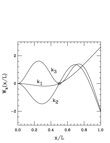
FIG. 14.: The first three modes for the discontinuous EHDI experiment. The circle indicates the pinning point $x_{p}/L=p/(p+q)$.

Otherwise stated, the total solvability condition is an average of those for (i) the left side clamped at $0$ and free at $x_{p}$, with the right side hinged at $x_{p}$ and free at $L$, and (ii) the left side clamped at $0$ and hinged at $x_{p}$, with the right side free at $x_{p}$ and free at $L$.

8 Initial data

Armed with a set of decaying modes, we may solve the equation for all times. We now attempt, as before, to construct a polynomial solution which describes the initial data. The polymer sits at rest with $y(0)=\Delta$ and is subject to the stated matching and boundary conditions. Noting that the shape must be described by polynomials of less than fourth order, since we wish to describe an elastica experiencing no forces, we find for the new polynomial $\bar{y}$

$${\bar{y}}^{a}\left(\alpha\right) = \Delta\left(1-{3\over 2}\alpha^{2}+{1\over 2}\alpha^{3}\right)$$ (147)

$${\bar{y}}^{f}\left(\sigma\right) = -\Delta{\frac{3\,\sigma}{2\,\rho}}~{}.$$ (148)

The final configuration, after the axoneme comes to rest and all transients have died, will be $-\bar{y}$: a third-order polynomial on the left and a straight line on the right. A pleasant fact is that this polynomial can also be derived by taking the limit as $v_{c}\rightarrow 0$ of $y_{0}h^{\{a,f\}}$.

9 Comparison with experiment

We now wish to use this information to arrive at a measurement of $A$. Hoping to verify the plausibility of this analysis, we compare with the results and accompanying model published with the experiment.

The model presented in [10] can be summarized as follows. First, the forces are calculated on a slender body subject to (i) a constant flow and (ii) a flow linearly increasing from $0$ at the origin to some $v_{m}$ at the end. The linearly-increasing flow describes that experienced by a rigidly rotating rod, in hopes that the force experienced by the actual (curved) filament, itself neither a straight rod, nor moving with constant velocity in time, is well-approximated. Curiously, different drag coefficients are used for these two forces.

The forces are then used to compute displacements, using the results for the elastica clamped at the origin, a condition which is unfortunately consistent with neither the assumption of a rodlike shape nor with the experimental geometry, in which the free side of the elastica is neither clamped ($y_{x}=0$, as was assumed for the calculation of displacement) nor hinged $(y_{xx}=0$, as might be considered appropriate for a straight rod); it is in fact experiencing a torque at $x_{p}$ due to the side of the filament between the trap and the axoneme.

Summing (i) the displacement $y_{c}(v_{c};\zeta_{1})$ of a clamped elastica in constant flow (using the first drag coefficient) and (ii) the displacement $y_{l}(v_{m};\zeta_{2})$ of an elastica subject to the linearly increasing flow it would have experienced were it a rigid rod (using the second drag coefficient), the total deflection $y_{\delta}$ from a straight line is obtained (see Eq. 20 of [10]):

$$y_{\delta}={\pi\eta(11v_{m}+30v_{c})l^{4}\over 60A\ln(2l/d)}.$$ (149)

It is then assumed that this displacement equals the deflection which would have been experienced had the filament not been initially horizontal, but rather constrained to some nonzero slope at the trap, specifically, that of the $t\rightarrow\infty$ solution for the shape, $-{\bar{y}}$.

This deflection $y_{\delta}$, from the right tip position at $t=\infty$ to that at $t=\Delta/v_{c}$, when the axoneme halts, is the first experimental observable. The second is the velocity at this tip at $t=\Delta/v_{c}$, which is then equated with the maximum velocity $v_{m}$ in the expression for $y_{l}$. Dividing $y_{\delta}$ by the weighted sum of velocities appearing in the numerator, one obtains the combination of two observables ($y_{\delta},v_{m}$) and one experimental parameter ($v_{c}$) which, according to this model, is equivalent to a simple quotient with units of time and in which $A$ appears explicitly,

$${\cal T}={y_{\delta}\over(11v_{m}+30v_{c})}={11\pi\eta\l^{4}\over{``A"}60\ln(2l/d)}$$ (150)

where ${``A"}$ indicates the rigidity which would be extracted from the data using this model. Note that the expression is a function only of $l$, the length of the free segment of the polymer. In this model, $l$ is taken to be “the hydrodynamically relevant length”[10].

Returning to the PDE-treatment of the problem, we see that the solutions to Eq. 119 for the long-time polynomial shape relate the velocity of the free end to the constant stage velocity as

$$v_{m}={v_{c}}h^{f}_{\tau}|_{\sigma=1}={3\over 2}{l\over x_{p}}v_{c}.$$ (151)

This simplification allows us to solve for the ratio in (149) of observables and parameters in terms of the polynomials in Eqs. 148 and 128.

$${\cal T}={\zeta l^{4}\over 2520{A}}{\frac{\left(-16\,{\rho}^{4}+210\,{\rho}^{2}+420\,\rho+231\right)}{\left(11+20\,\rho\right)}}$$ (152)

where ${A}$ indicates the value of the bending modulus which one would calculate had one used the same data and thus the same quotient ${\cal T}$.

The ratio ${A}/{``A"}$ is a simple expression and allows us to compare by what factor this differential equation-based analysis differs from the published model given some experimental data ${\cal T}(l)$. Equating the two expressions for ${\cal T}$ and isolating ${A}/{``A"}$, we find

$${{A}\over{``A"}}=2{\ln({L\over d}{1\over 2(1+\rho)})\over\ln({L\over d}{4\over\sqrt{e}})}\left(1+{{210\rho^{2}-16\rho^{4}}\over{231+420\rho}}\right)$$ (153)

where we have moved the ${\cal O}(1)$ constants into the argument of the logarithm for compactness. The dominant behavior is captured by the polynomial dependence on $\rho$, but we can see that the function will be $\sim 2$, indicating a systematic underestimate by the published model of the bending modulus. A plot of the ratio, with typical values taken from experiment, is shown in Fig. 15.

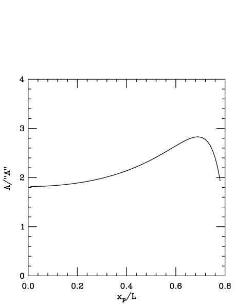
FIG. 15.: Quotient of values derived for the bending modulus using the model of [10] and that presented herein.

Note that we have arrived at this expression by ignoring the transient component in the exact expression. This is valid only in the range where the polynomial (asymptotic) solution dominates over the transients, a condition which is violated above $\rho\simeq 4,x_{p}/L=\rho/(\rho+1)\simeq 0.8$.

We expect then, for results obtained with the model in [10] systematically to underestimate the bending modulus $A$ by a factor $\sim 1/2$. In fact, we can fit the published values of ${\cal T}(l)$ via nonlinear $\chi^{2}$ fitting to arrive at a value for A. Unfortunately, the incorporation of the effects due to the left end of the polymer introduces a dependence on $L$, data for which are unpublished. Unable to elicit a response from the authors regarding the total lengths used in the experiment, we could only fit for both parameters. The analysis produced lower $\chi^{2}$ values than the model of [10]; however, $\chi^{2}$ is extremely weakly-dependent on $L$ and not a particularly advantageous method without this datum. In each case, the fit values of $A$ were approximately twice that reported in [10].

VIII Conclusions

We have attempted to show that a systematic treatment of linearized elastohydrodynamics for filamentous biopolymers can be formulated with fruitful results. Specifically, we anticipate these methods should be useful in the design and analysis of dynamic experiments. Further, we have proposed a new technique (EHDII) which exploits viscous hydrodynamics to extend the range of mechanical experiments of bending moduli to more flexible polymers. We expect this experiment to produce more accurate results when repeated with lower-amplitude driving, and thereby help determine conclusively the existence or nonexistence of scale-dependent or time-dependent elastic behaviors in biopolymers as well as the value of $A$ in in vitro assays. It is our hope that the analysis associated with this experiment will also encourage renewed interest in the problems of flagellar motion and slender-body hydrodynamics in general.

Moreover, we have seen that attentiveness to equations of motion and boundary conditions for the elastica has measurable consequences, and that construction of the appropriate function space associated with these conditions leads to a pleasant union of mathematical and physical consequences, quantifying our intuitions and relating transcendental equations to physical effects and experimental observables. We believe that the significance of boundary conditions and the natural function space for the elastica has been overlooked in existing treatments of the dynamics and statistical mechanics relevant to experiments being performed and discussed by the community.

We look forward to the extension of this analysis to arbitrary geometries, reflecting distortions beyond small order and hydrodynamics beyond the lowest-order approximation of slender-body flow. Though the exact equation of motion is nonlinear, the Stokesian dynamic and the vanishing of successive derivatives remain, and we expect the mechanisms and effects which we have outlined here to persist.

Natural extensions of this research include nonplanar geometries and the incorporation of twist. These would be complementary to recent work on the Hamiltonian dynamics of twisted elastic rods [14, 25]. The dynamics of twist are especially intriguing in the light of recent work on twist-bend coupling [15] and the proposal that this coupling creates scale-dependent elasticity in actin [16]. Another intriguing experimental realization of nonplanar viscous elastohydrodynamics with twist is the supercoiling of fibers of mutants of the common bacterium Bacillus subtilis [24]. We are currently formulating the analysis appropriate to these promising applications, armed with the lessons learned in this investigation.

IX Acknowledgments

We thank Steve Block and Steve Gross for early discussions on analysis of the data and for bringing [10] to our attention, and Joseph Käs for pointing out [12]. We also thank Almut Bruchard, Mark Johnson, Frank Jülicher, Randall Kamien, David Levermore, Mike Shelley, and especially Tom Powers for useful conversations and insight. This work was supported by NSF PFF Grant DMR 93-50227 and the A.P. Sloan Foundation (REG).

A Eigenfunctions of $\partial_{\alpha}^{4}$

If we equate functions related by the reflection $\alpha\rightarrow 1-\alpha$, there are $4(4+1)/2=10$ distinct eigenfunctions of $\partial_{\alpha}^{4}$, determined by boundary conditions, for which this operator is self-adjoint. Each has an associated solvability condition for the eigenvalues $k$. We list the solvability conditions and the unnormalized eigenfunctions, indexed according to the conditions at the ends:

$$\left(f\right) {\rm free}: h_{xx}=h_{xxx}=0$$ (A1)

$$\left(c\right) ~{}{\rm clamped}:~{} h=h_{x}=0$$ (A2)

$$\left(h\right) {\rm hinged}: h=h_{xx}=0$$ (A3)

$$\left(t\right) ~{}{\rm torqued}:~{} h_{xxx}=h_{x}=0$$ (A4)

The general solution is ${\cal W}_{k}=a_{1}\cos k\alpha+a_{2}\sin k\alpha+a_{3}\cosh k\alpha+a_{4}\sinh k\alpha$, where $\alpha\in(0,1)$. The letters f,c,h,t denote the boundary conditions at the left and right. Note that for special cases, the calculated ${\cal W}_{k}$ are merely a Fourier basis.

$$\bullet{\rm f-f}:$$ (A8)

$$\cos k\cosh k=1;$$

$${\cal W}_{k}=\left(\sin k\alpha+\sinh k\alpha\right)\left(\sin k+\sinh k\right)$$

$$~{}+\left(\cos k\alpha+\cosh k\alpha\right)\left(\cos k-\cosh k\right)$$

$$\bullet{\rm c-c}:$$ (A12)

$$\cos k\cosh k=1;$$

$${\cal W}_{k}=\left(\sin k\alpha-\sinh k\alpha\right)\left(\sin k+\sinh k\right)$$

$$~{}+\left(+\cos k\alpha-\cosh k\alpha\right)\left(\cos k-\cosh k\right)$$

$$\bullet{\rm f-c}:$$ (A16)

$$\cos k\cosh k=-1;$$

$${\cal W}_{k}=\left(\sin k\alpha+\sinh k\alpha\right)\left(\sin k-\sinh k\right)$$

$$~{}+\left(\cos k\alpha+\cosh k\alpha\right)\left(\cos k+\cosh k\right)$$

$$\bullet{\rm h-h}:$$ (A19)

$$\sin k=0;$$

$${\cal W}_{k}=\sin k\alpha$$

$$\bullet{\rm t-t}:$$ (A22)

$$\sin k=0;$$

$${\cal W}_{k}=\cos k\alpha$$

$$\bullet{\rm h-t}:$$ (A25)

$$\cos k=0;$$

$${\cal W}_{k}=\sin k\alpha$$

$$\bullet{\rm f-h}:$$ (A29)

$$\tan k=\tanh k;$$

$${\cal W}_{k}=\left(\sin k\alpha+\sinh k\alpha\right)\left(-\cos k+\cosh k\right)$$

$$~{}+\left(\cos k\alpha+\cosh k\alpha\right)\left(\sin k-\sinh k\right)$$

$$\bullet{\rm f-t}:$$ (A33)

$$\tan k=-\tanh k;$$

$${\cal W}_{k}=\left(\sin k\alpha+\sinh k\alpha\right)\left(\sin k+\sinh k\right)$$

$$~{}+\left(\cos k\alpha+\cosh k\alpha\right)\left(\cos k-\cosh k\right)$$

$$\bullet{\rm c-t}:$$ (A37)

$$\tanh k=-\tanh k;$$

$${\cal W}_{k}=\left(\sin k\alpha-\sinh k\alpha\right)\left(\sin k+\sinh k\right)$$

$$~{}+\left(\cos k\alpha-\cosh k\alpha\right)\left(\cos k-\cosh k\right)$$

$$\bullet{\rm c-h}:$$ (A41)

$$\tan k=\tanh k;$$

$${\cal W}_{k}=\left(\sin k\alpha-\sinh k\alpha\right)\left(\cos k+\cosh k\right)$$

$$~{}+\left(-\cos k\alpha+\cosh k\alpha\right)\left(\sin k+\sinh k\right)$$

B Properties of the ${\cal W}_{\rm k}$ basis

We define ${\cal W}_{k}$ by the operator of which it is an eigenfunction and by its boundary conditions:

$${\cal H}\equiv\partial_{\alpha}^{4}~{}+{\rm boundary~{}conditions}.$$ (B1)

Next we establish the self-adjointness of ${\cal H}$, which we may express in Dirac notation as $\langle{\cal W}_{k}|{\cal H}{\cal W}_{j}\rangle=\langle{\cal H}{\cal W}_{k}|{\cal W}_{j}\rangle$. This follows from the integration

$$\int_{0}^{1}\!d\alpha{\cal W}_{k}\partial_{\alpha}^{4}\left({\cal W}_{j}\right) = \int_{0}^{1}\!d{\alpha}\partial_{\alpha}^{4}\left({\cal W}_{k}\right){\cal W}_{j}$$ (B4)

$$+{\cal W}_{k}\partial_{\alpha}^{3}{\cal W}_{j}\bigl{|}_{0}^{1}-\partial_{\alpha}^{1}{\cal W}_{k}\partial_{\alpha}^{2}{\cal W}_{j}\bigl{|}_{0}^{1}$$

$$+\partial_{\alpha}^{2}{\cal W}_{k}\partial_{\alpha}^{1}{\cal W}_{j}\bigl{|}_{0}^{1}-\partial_{\alpha}^{3}{\cal W}_{k}{\cal W}_{j}\bigl{|}_{0}^{1}$$

$$= \int_{0}^{1}\!d{\alpha}\partial_{\alpha}^{4}\left({\cal W}_{k}\right){\cal W}_{j}~{},\ \ \ \ \Box$$ (B5)

where all the surface terms are seen to disappear for any choice of boundary conditions from appendix A.

We can also establish the orthogonality of the members of a family since

$$\int_{0}^{1}d\alpha{\cal W}_{j}{\cal W}_{k} = \int_{0}^{1}d\alpha{\cal W}_{j}{\partial_{\alpha}^{4}{\cal W}_{k}\over k^{4}}=k^{-4}\int_{0}^{1}d\alpha\partial_{\alpha}^{4}{\cal W}_{j}{\cal W}_{k}$$ (B6)

$$= \Bigl{(}{j\over k}\Bigr{)}^{4}\int_{0}^{1}d\alpha{\cal W}_{j}{\cal W}_{k}~{}.$$ (B7)

Thus $\int_{0}^{1}d\alpha{\cal W}_{j}{\cal W}_{k}=0$ for $j\neq k$.

We justify considering only real, positive values of $k^{4}$ by observing

$$k^{4}\int_{0}^{1}d\alpha{\cal W}_{k}{\cal W}_{k}^{*} = \int_{0}^{1}d\alpha\partial_{\alpha}^{4}{\cal W}_{k}{\cal W}_{k}^{*}$$ (B8)

$$= \partial_{\alpha}^{3}{\cal W}_{k}{\cal W}_{k}^{*}|_{0}^{1}d\alpha-\partial_{\alpha}^{2}{\cal W}_{k}\partial_{\alpha}^{1}{\cal W}_{k}^{*}|_{0}^{1}d\alpha$$ (B10)

$$+\int_{0}^{1}d\alpha\partial_{\alpha}^{2}{\cal W}_{k}\partial_{\alpha}^{2}{\cal W}_{k}^{*}$$

so

$$k^{4}={\int_{0}^{1}d\alpha|\partial_{\alpha}^{2}{\cal W}_{k}|^{2}\over\int_{0}^{1}d\alpha|{\cal W}_{k}|^{2}}~{},$$ (B11)

the quotient of two real, positive quantities, which is necessarily real and positive.

C Exact solution to EHD problem II

The exact solution to EHDII can be written in somewhat compact form at the cost of introducing new definitions. Employing the parameter $\alpha\equiv x/L$, the rescaled length ${\cal L}\equiv L/\ell$, and the constant $z_{0}=exp(-i\pi/8)$ as in Eq. 73, we introduce

$$\xi\equiv{\rm e}^{z_{0}{\cal L}}$$ (C1)

and then write

$$h(\alpha,{\cal L})\equiv h_{\infty}(\alpha)+h_{\flat}(\alpha,{\cal L})~{}.$$ (C2)

where $h_{\infty}$ is the semiinfinite solution, and $h_{\flat}\rightarrow 0$ as ${\cal L}\to\infty$. Explicitly,

$$h_{\flat}={1\over 2}C_{1}\left(\xi^{\alpha}-\xi^{-\alpha}\right)+{1\over 2}C_{2}\left(\xi^{i\alpha}-\xi^{-i\alpha}\right)~{},$$ (C3)

where

$$C_{1}({\cal L}) = \xi^{-1}{(-i\xi^{-i}-\xi^{i}+(1+i)\xi)\over(i\xi^{-1-i}+\xi^{-1+i}-\xi^{1-i}-i\xi^{1+i})}$$ (C4)

$$C_{2}({\cal L}) = \xi^{-i}{(i\xi^{-1}-\xi^{1}+(1-i)\xi^{i})\over(-i\xi^{-1-i}-\xi^{-1+i}+\xi^{1-i}+i\xi^{1+i})}~{},$$ (C5)

and

$$h_{\infty}={1\over 2}\left(\xi^{-\alpha}+\xi^{-i\alpha}\right).$$ (C6)

D Solvability condition for discontinuous EHDI

Associated with the discontinuous EHDI problem is the set of eigenvalues of $\partial_{\alpha}^{4}$ appropriate to the boundary and matching conditions. Like the statement $\sin(kL)=0$ for determining the allowed Fourier $k$ values for a doubly-hinged filament of length $L$, there is a solvability condition for $p\equiv kx_{p}$ , $q\equiv k\left(L-x_{p}\right)=kl$, derived by setting the determinant of an $8$ by $8$ matrix to $0$, an equation which can be written:

$$0 = {\cal D}\left(p,q\right)=$$ (D7)

$$-\sin\left(q\right)\cos\left(p\right)\cosh\left(q\right)\cosh\left(p\right)$$

$$-\cos\left(q\right)\sin\left(p\right)\cosh\left(q\right)\cosh\left(p\right)$$

$$+\cos\left(q\right)\cos\left(p\right)\sinh\left(q\right)\cosh\left(p\right)$$

$$+\cos\left(q\right)\cos\left(p\right)\cosh\left(q\right)\sinh\left(p\right)$$

$$-\sin\left(q\right)\cosh\left(q\right)+\cos\left(q\right)\sinh\left(q\right)$$

$$+\sin\left(p\right)\cosh\left(p\right)-\cos\left(p\right)\sinh\left(p\right)$$

The ratio $x_{p}/(L-x_{p})=q/p=\rho$, set by the geometry of the experiment, fixes a diagonal line passing through the origin and intersecting the set of curves defined by this equation to define all the allowed $k$ values, as illustrated in Fig. 13.

REFERENCES

- [1] Amblard, F., A. C. Maggs, B. Yurke, A. N. Pargellis, and S. Leibler. 1996. Subdiffusion and anomalous local viscoelasticity in actin networks. Phys. Rev. Lett. 77:4470-4473.
- [2] Antman, S. S. 1995. Nonlinear Problems of Elasticity. Springer-Verlag, New York.
- [3] Brower, R., D. A. Kessler, J. Koplik, and H. Levine. 1984. Geometrical models of interface evolution. Phys. Rev. A 29:1335-1342.
- [4] Childress, S. 1981. Swimming and Flying in Nature. Cambridge University Press, Cambridge.
- [5] Cluzel, P., A. Lebrun, C. Heller, R. Lavery, J. L. Viovy, D. Chatenay, and F. Caron. 1996. DNA: an extensible molecule, Science 271:792-794.
- [6] Cox, R. 1970. The motion of long slender bodies in a viscous fluid: Part I. General theory. J. Fluid Mech. 44:791-810.
- [7] Cox, R. 1970. The motion of long slender bodies in a viscous fluid: Part II. Shear flow. J. Fluid Mech. 45:625-657.
- [8] Cross, M. C. and P. C. Hohenberg. 1993. Pattern formation outside of equilibrium. Reviews of Modern Physics 65:851-1112.
- [9] Doi, M. and S. F. Edwards. 1986. The Theory of Polymer Dynamics. Clarendon Press, Oxford.
- [10] Felgner, H., R. Frank and M. Schliwa. 1996. Flexural rigidity of microtubules measured with the use of optical tweezers. J. Cell Sci. 109:509-516.
- [11] Feynman, R. 1962. Lectures in Physics II. Addison-Wesley Publishing, New York.
- [12] Gittes, F., B. Mickey, J. Nettleton, and J. Howard. 1993. Flexural rigidity of microtubules and actin filaments measured from thermal fluctuations in shape. J. Cell. Biol. 120:923-934.
- [13] Goldstein, R. and S. Langer. 1995. Nonlinear dynamics of stiff polymers. Phys. Rev. Lett. 75:1094-1097.
- [14] Goriely, A. and M. Tabor. 1996. Nonlinear dynamics of filaments I: Dynamical instabilities (Accepted for publication in Physica D).
- [15] Kamien, R. 1997. Local writhing dynamics. http://xxx.lanl.gov/abs/cond-mat/9703137.
- [16] Käs, J., H. Strey, M. Baermann, and E. Sackmann. 1993. Direct measurement of the wave-vector-dependent bending stiffness of freely flickering actin filaments. Europhys. Lett. 21:865-870.
- [17] Keller, J. and S. Rubinow. 1976. Slender-body theory for slow viscous flow. J. Fluid Mech. 44:705.
- [18] Kurachi, M., M. Hoshi, and H. Tashiro. 1995. Buckling of a single microtubule by optical trapping forces: direct measurement of microtubule rigidity. Cell Motil Cytoskeleton, 30:221-228.
- [19] Landau, L. and L. Lifshitz. 1987. Fluid Mechanics, Pergamon, New York. p 59.
- [20] Lighthill, Sir J. 1975. Mathematical Biofluiddynamics. SIAM, Philadelphia.
- [21] Love, A. E. H. 1892. A Treatise on the Mathematical Theory of Elasticity. Cambridge University Press, Cambridge.
- [22] Machin, K. E. 1958. Wave propagation along flagella. J. Exp. Biol. 35:796-806.
- [23] Machin, K. E. 1962. The control and synchronization of flagellar movement. Proc. Roy. Soc. B 62:88-104.
- [24] Mendelson, N. H. 1990. Bacterial macrofibers: the morphogenesis of complex multicellular bacterial forms. Sci. Progress Oxford, 74:425-441.
- [25] Olson, W. K. and Zhurkin, V. B. 1996. Twenty years of DNA bending. In Biological Structure and Dynamics, Vol. 2. R. H. Sarma and M. H. Sarma, editors. Adenine Press, Schenectady. 341-370.
- [26] Ott, A., M. Magnasco, A. Simon, and A. Libchaber. 1993. Measurement of the persistence length of polymerized actin using florescence microscopy. Phys. Rev. E 48:1642-1645.
- [27] Pardee, J. D., and J. A. Spudich. 1982. Purification of muscle actin. Methods Enzymol. 85B:164-181.
- [28] Purcell, E. M. 1977. Life at low Reynolds number, Am. J. Phys. 45:3-11.
- [29] Shelley, M. J. and T. Ueda. 1996. The nonlocal dynamics of stretching, buckling filaments. In Advances in Multi-fluid Flows. Y. Y. Renardy, A. V. Coward, D. T. Papageorgiou, and S-M Sun, editors. AMS-SIAM, Philadelphia. 415-425.
- [30] Smith, S. B., Y. Cui, C. Bustamante. 1996. Overstretching B-DNA: the elastic response of individual double-stranded and single-stranded DNA molecules. Science. 271:795-799.
- [31] Stokes, G.G. 1851. Mathematical and Physical Papers III. Cambridge University Press, Cambridge. 19, 130.
- [32] Taylor, G. 1952. The action of waving cylindrical tails in propelling microscopic organisms. Proc. Roy. Soc. A 217:225-239.
- [33] Vernier, P., A.C. Maggs, M.-F. Carlier, and D. Pantaloni. 1994. Analysis of microtubule rigidity using hydrodynamic flow and thermal fluctuations, J. Biol. Chem. 269:13353-13360.
- [34] Weinstock, R. 1974. Calculus of Variations. Dover, New York.
- [35] Wiggins, C. 1974. Biopolymer Euler buckling. In preparation.
- [36] Wilczek, F. and A. Shapere. 1987. Self-propulsion at low Reynolds number. Phys. Rev. Lett. 58:2051-2053.
- [37] Yin, H., M. D. Wang, K. Svoboda, S. M. Block, and J. Gelles. 1995. Transcription against an applied force, Science 270:1653-1657.