Effect of Gravity and Confinement on Phase Equilibria:
A Density Matrix Renormalization Approach

Abstract

The effect of gravity on a two dimensional fluid, or Ising magnet, confined between opposing walls is analyzed by density matrix renormalization. Gravity restores two phase coexistence up to the bulk critical point, in agreement with mean field calculations. A detailed finite size scaling analysis of the critical point shift is performed. Density matrix renormalization results are very accurate and the technique is promising and best suited to study equilibrium properties of two dimensional classical systems in contact with walls or with free surfaces.

The thermodynamical properties of confined systems have received a lot of attention in the past years [1, 2, 3, 4, 5, 6, 7, 8, 9, 10]. Their critical behavior is rather different from the bulk criticality and has been the subject of extended investigations by means of mean field and scaling analysis [1, 2, 3, 4], Monte Carlo simulations [5, 6, 7, 8] and exact calculations [9, 10]. The simplest and most studied case is the Ising model in a $L\times M^{d-1}$ lattice with $M\to\infty$, i.e. confined between two infinite walls separated by a finite distance $L$. Of considerable interest is the situation in which magnetic fields ($h_{1}$ and $h_{2}$) acting on the spins at the walls are introduced.

For parallel surface fields ($h_{1}\cdot h_{2}>0$) and finite $L$ two phase coexistence is shifted to finite values of a bulk magnetic field $h$ [1], as illustrated in Fig. 1(a). This phenomenon is analogous to the capillary condensation for a fluid confined between two parallel surfaces, where the gas-liquid transition occurs at a lower pressure than in the bulk. Finite size scaling [1] predicts that the capillary critical point $[h_{c}(L),T_{c}(L)]$ scales as:

$$T_{c}(L)-T_{c}\sim L^{-y_{T}}\,\,\,\,\,\,\, \,\,\,\,\,\,\,h_{c}(L)\sim L^{-y_{H}},$$ and (1)

where $T_{c}$ is the bulk critical temperature and $y_{T}=1/\nu$, $y_{H}=d-\beta/\nu$ are the thermal and magnetic exponents, respectively (here $d$ is the dimensionality, $\nu$ and $\beta$ are the correlation length and magnetization exponents, respectively).

At fixed $T<T_{c}$ and finite $L$ the scaling to the first order line is of type [1]:

$$h_{0}(L)\sim 1/L.$$ (2)

While the previous relation has been verified in Monte Carlo simulations in $d=2,3$ [6, 7], a direct verification of the scaling of the capillary critical point has not been attempted yet, due to the high computational effort [7] needed to locate accurately $[h_{c}(L),T_{c}(L)]$.

The case of opposing surface fields (for simplicity we consider $h_{1}=-h_{2}$) was analyzed in detail by Parry and Evans [2] using a Ginzburg-Landau approach. They found that two phase coexistence is restricted to temperatures below the interface delocalization temperature $T_{d}(L)$ as shown in Fig. 1(a); the surprising result [2] is that $T_{d}(L)$ does not scale to the bulk point $T_{c}$, for $L\to\infty$, but to the wetting temperature $T_{w}$ as:

$$T_{d}(L)-T_{w}\sim L^{-1/\beta_{s}}.$$ (3)

Here $\beta_{s}$ is the exponent describing the divergence of the thickness of the wetting layer for a semi infinite system: $l\sim(T_{w}-T)^{-\beta_{s}}$. We recall also that $T_{w}$ depends on the value of the surface field $h_{1}$ and can be far away from the bulk critical point (see Fig. 1(b)). For $T_{d}(L)\leq T<T_{c}$ there is a single phase [2], with an interface meandering freely between the walls. Numerical results from extensive Monte Carlo simulations [5, 8] in $d=2,3$ confirm the mean field scenario.

FIG. 1.: (a) Phase diagram of the d-dimensional Ising model for a bulk system in the (h,T) plane (solid line). The dashed lines are the phase diagrams of confined systems with identical (1) and opposing (2) surface fields. (b) Dependence of the wetting temperature on the surface field $h_{1}$.

Rogiers and Indekeu [4] extended the model with opposing surface fields, including a bulk field which varies linearly along the finite direction of the system and models the effect of gravity on a confined fluid. They considered the following Hamiltonian:

$$H = -J\sum_{(i,j)}s_{(i,j)}s_{(i+1,j)}-J\sum_{(i,j)}s_{(i,j)}s_{(i,j+1)}+h_{1}\sum_{j}s_{(1,j)}-h_{1}\sum_{j}s_{(L,j)}+g\sum_{i=1}^{L}(2i-1-L)\sum_{j}s_{(i,j)},$$ (4)

where $J>0$, $s_{(i,j)}=\pm 1$ and $1\leq i\leq L$ labels the lattice sites along the finite direction, while $j$ labels the remaining $d-1$ directions. The parameter $g$ is the equivalent of the gravitational constant. Using a mean field approach, it was found [4] that the ordinary scaling to the bulk critical point is restored in an extended parameter space where $g$ is included. While the mean field analysis is correct at dimensions higher than the upper critical dimension ($d=4$), its validity in lower dimensions, where thermal fluctuations become important, is questionable.

The aim of this Letter is to study the phase diagram of the model described by the Hamiltonian (4) for an $L\times\infty$ strip, beyond the mean field approximation. We test the validity of the conclusions of Ref. [4] at the lower critical dimension ($d=2$) and clarify the mechanism of the critical point shift for a system confined between opposing walls. We analyze also the exponents governing this shift and test the validity of scaling assumptions that have been proposed some time ago [1, 11], but, to our knowledge, never derived directly from a microscopic model.

The numerical calculations are based on a density matrix renormalization group (DMRG) approach, a technique developed by White [12, 13] for the study of ground state properties of quantum spin chains. Nishino [14] extended the DMRG to $d=2$ classical systems as a transfer matrix renormalization. Transfer matrices are frequently used for numerical investigations of $L\times\infty$ strips; computations are restricted to small strip widths since the dimension of the transfer matrix grows exponentially with $L$ [15]. In the DMRG algorithm one constructs effective transfer matrices of small dimensions (i.e. numerically tractable), but which describe strips of large widths. The spin space is truncated in a very efficient manner and the numerical accuracy is very good [12, 13, 14], even for renormalized matrices of not too large dimensions [16]. More details will be presented elsewhere [17].

We start the analysis of the phase diagram of the model from its ground state properties. At $T=0$, $h_{1}<J$ and for a strip of width $L$ the ground state is double degenerate (two phase coexistence) with all spins either up or down for:

$$\frac{4}{L^{2}}(h_{1}-J)\,\,\leq\,\,g\,\,\leq\,\,\frac{4}{L^{2}}(h_{1}+J)$$ (5)

For values of $g$ outside this interval the ground state is non degenerate, with an infinitely long straight interface at the center of the strip separating a region with all spins up from a region with all spins down.

To distinguish the two phase coexistence region from a single interface-like state it is convenient to calculate the correlation function between two neighboring spins at the center of the strip $c_{L/2}\equiv\langle s_{\left(\frac{L}{2},j\right)}s_{\left(\frac{L}{2}+1,j\right)}\rangle$. At $T=0$, $c_{L/2}$ drops from $+1$ in the two phase coexistence region to $-1$ in the single phase region. For nonzero temperatures, a sharp distinction between these two regions is not possible since true criticality does not occur for finite values of $L$. However a peak in the temperature derivative of $c_{L/2}$ can be seen as a pseudocritical point where the system goes through a smooth change from two phase coexistence to a one phase state, without a true phase transition. As the strip width increases these finite peaks shift towards the true thermodynamic singularities of the bulk system. The analysis of shifts of pseudocritical points has been considered already [3, 5] for the present model in absence of gravity.

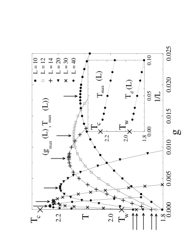
FIG. 2.: Phase diagram of the model for different strip widths in the ($g,T$) plane for $h_{1}=0.5$ and $J=1$; the area below the curves is the two phase coexistence region. Inset: Scaling of $T_{\rm{max}}(L)$ and $T_{d}(L)$ vs $1/L$. Error bars are much smaller than symbol sizes.

Figure 2 shows the phase diagram in the $(g,T)$ plane for $J=1$, $h_{1}=0.5$. Each curve is the phase boundary between the two phase coexistence (area below the curve) and the one phase region, for a specific value of $L$. Only the phase boundaries for $L$ up to $40$ are shown although the largest size considered is $L=60$. For $g>0$ two phase coexistence is shifted to higher temperatures with respect to $g=0$ due to a competing effect of surface and bulk fields, while at negative $g$ phase coexistence is suppressed. As $L$ increases the whole two phase coexistence region shrinks and shifts towards the $g=0$ axis. The intersections of the phase boundaries with this axis, indicated by the horizontal arrows in Fig. 2, define the interface delocalization transition temperatures $T_{d}(L)$; the phase boundary maxima $[g_{\rm{max}}(L)$,$T_{\rm{max}}(L)]$ are indicated by the vertical arrows in the figure.

FIG. 3.: Plot of $\ln[g_{\rm{max}}(L)]$ vs $\ln L$ for different surface fields. The dotted lines correspond to a slope $-2.875$. Error bars are smaller than symbol sizes.

We find for $T_{d}(L)$ a scaling in excellent agreement with Eq. (3) [5, 8] and for $T_{\rm max}(L)$ a scaling of the type:

$$T_{\rm max}(L)-T_{c}\sim L^{-y_{T}}$$ (6)

with the $d=2$ Ising exponents $\beta_{s}=1$ and $y_{T}=1$. A plot of $T_{\rm{max}}(L)$ and $T_{d}(L)$ for $h_{1}=0.5$ as function of $1/L$ is shown in the inset of Fig. 2. From an extrapolation of the data in the figure we find the following estimates for the wetting and bulk critical temperatures: $T_{w}=1.9584(8)$ and $T_{c}=2.272(4)$ (the exact values are $T_{w}=1.95845$ [18] and $T_{c}=2.269$). The same scaling analysis has been extended to several values of $h_{1}$: all data points are in excellent agreement with the relations (3) and (6).

Van Leeuwen and Sengers [11] analyzed the influence of gravity in an infinitely extended system; they argued that the product of $g$ with a length in the direction of the gravitational field should scale as a bulk constant field. On a finite strip, this leads to the following scaling prediction [4]:

$$g_{\rm{max}}(L) \sim L^{-\left(1+y_{H}\right)}.$$ (7)

Both at $T=0$ (see inequality (5)) and also for finite $T$ [17], not too close to the phase boundary maxima, we find a scaling towards the bulk first order line of type $1/L^{2}$, in agreement with Van Leeuwen and Sengers’ conjecture since the corresponding scaling of a constant bulk field is $1/L$ (see (2)).

Figure 3 shows a plot of $\ln[g_{\rm{max}}(L)]$ vs $\ln(L)$ for four values of $h_{1}$, from $0.1$ to $0.99$ and $J=1$ [19]. The dotted lines, drawn as a guide to the eye, correspond to a scaling of type (7) with the $d=2$ Ising exponent $1+y_{H}=2.875$. The data agree with the scaling relation (7) for the largest surface field considered ($h_{1}=0.99$) for which a linear fit of the points for $L\geq 20$ yields an exponent $2.86(2)$ in good agreement with the Ising value. At lower surface fields and up to the largest size considered ($L=60$) the exponent deviates from the expected value and increases from $2.4$ to $2.6$ as the surface field increases from $h_{1}=0.1$ to $h_{1}=0.5$. The scaling analysis for $g_{\rm max}(L)$ is somewhat more problematic than the scaling of $T_{\rm max}(L)$; this was to be expected since along the gravitational field direction there is a scaling to $T_{c}$ and a scaling to the bulk first order line (of type $1/L^{2}$). The interplay between these two scalings may be the cause of the observed shift of the exponent of $g_{\rm max}(L)$ from the Ising value for low surface fields, where the asymptotic behavior (7) possibly sets in for $L\gg 60$. In other studies of confined systems it was found that, in the scaling analysis of finite size data, the value of the system width beyond which one has a clear asymptotic behavior, may depend strongly on the surface field (see for instance Ref.[7]).

Figure 4 shows some magnetization profiles for $L=60$, $J=1$, $h_{1}=0.5$, $T=2.0$ and for different values of $g$. The profile (a) corresponds to a point of the phase diagram located in the two phase coexistence region, where the magnetization is averaged over two phases. This profile is similar to those calculated exactly by Maciołek and Stecki [10, 20] for $g=0$ and $T<T_{d}(L)$. Profiles (b) and (c) correspond to points of the phase diagram in the one phase region. Notice the competing effect between gravity and surface fields in the vicinity of the walls in the profile (b).

Magnetization profiles of interface-like configurations can be calculated using a solid-on-solid (SOS) approximation [21]. It is assumed that all the spins at the two sides of the interface are fixed and take values $\pm m_{0}$; interfacial configurations with overhangs are neglected.

SOS magnetization profiles are shown in Fig. 4 (dashed lines) and are given by [17]:

$$\langle s_{(i,j)}\rangle=\frac{2m_{0}}{\sqrt{\pi}}\,\,\int_{0}^{x(i)/\xi_{\perp}}dt\,\,e^{-t^{2}},$$ (8)

where $x(i)=L[i-(L+1)/2]/(L-1)$ and $\xi_{\perp}$, the interface width, is given by the relation:

$$\xi_{\perp}=\sqrt{\frac{T}{2\sqrt{|g|m_{0}\sigma_{0}}}}.$$ (9)

with $\sigma_{0}$ the surface tension. For $\sigma_{0}$ and $m_{0}$ we take their exactly known values at $g=0$; this approximation is good for low gravity.

Results from the interface Hamiltonian agree well with those calculated with DMRG even at temperatures not too far from $T_{c}$ (in Fig. 4 the temperature is approximately $10\%$ below $T_{c}$). Gravity has the effect of reducing interface fluctuations, so that configurations with overhangs, which are not taken into account in the SOS model, have small weights. We stress that (8) is valid in the limit $\xi_{\perp}\ll L$ since the effect of the walls has been neglected.

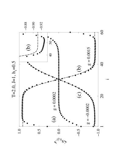
FIG. 4.: (Circles) Magnetization profiles in the two phase coexistence region (a) and in the single phase region ((b) and (c)) calculated by DMRG. (Dashed lines) Profiles calculated with a SOS approximation [Eq. 8]. Inset: Detail of the profile (b) far from the interfacial region.

In conclusion, we found that the competing effects of surface fields and gravity restore the “ordinary” finite size scaling to the bulk critical point, in agreement with mean field predictions [4], which thus survive the strong thermal fluctuations at the lower critical dimension. It is currently believed that the model confined between opposing walls is “special” because of the peculiar critical point shift (3) which is somewhat anomalous and has attracted a lot of interest in recent years [2, 3, 5, 8, 22]. In our opinion this point of view needs to be reconsidered; the mechanism of critical point shift becomes clear only for nonzero gravity where we find a scaling relation (6) completely analogous to that expected for the capillary critical point (1).

Although they are currently restricted to two dimensions, DMRG techniques provide accurate results for studying equilibrium properties of large systems. The fact that the DMRG accuracy is the best for open boundary conditions [12, 13] and that transfer matrices describe strips that are infinite along the transfer direction make the method best suited to study systems in contact with walls or with free surfaces.

We are grateful to J.O. Indekeu for suggesting us the topic of this Letter and for several discussions. Stimulating discussions with C. Boulter, R. Dekeyser, A.O. Parry and J. Rogiers are gratefully acknowledged. E.C. was supported by E.C. Human Capital and Mobility Programme N. CHBGCT940734. During his stay in Leuven A.D. was supported by the K.U. Leuven Research Fund (F/95/21).

REFERENCES

- [1] M. E. Fisher and H. Nakanishi, J. Chem. Phys. 75, 5857 (1981); H. Nakanishi and M. E. Fisher, J. Chem. Phys. 78, 3279 (1983).
- [2] A. O. Parry and R. Evans, Phys. Rev. Lett. 64, 439 (1990).
- [3] A. O. Parry and R. Evans, Physica 181 A, 250 (1992).
- [4] J. Rogiers and J. O. Indekeu, Europhys. Lett. 24, 21 (1993).
- [5] E. V. Albano, K. Binder, D.W. Heermann and W. Paul, Surf. Sci. 223, 151 (1989).
- [6] E. V. Albano, K. Binder, D.W. Heermann and W. Paul, J. Chem. Phys. 91, 3700 (1989).
- [7] K. Binder and D. P. Landau, J. Chem. Phys. 96, 1444 (1992).
- [8] K. Binder, D. P. Landau and A. M. Ferrenberg, Phys. Rev. Lett. 74, 298 (1995); Phys. Rev. E 51, 2823 (1995).
- [9] M. E. Fisher and H. Au-Yang, Physica (Utrecht) 101, 255 (1980); H. Au-Yang and M. E. Fisher, Phys. Rev. B 21, 3956 (1980).
- [10] A. Maciołek and J. Stecki, Phys. Rev. B 54, 1128 (1996).
- [11] J. M. J. van Leeuwen and J. V. Sengers, Physica 128 A, 99 (1984); Physica 138 A, 1 (1986).
- [12] S. R. White, Phys. Rev. Lett. 69, 2863 (1992).
- [13] S. R. White, Phys. Rev. B 48, 10345 (1993).
- [14] T. Nishino, J. Phys. Soc. Jpn. 64, 3598 (1995).
- [15] For instance, for an Ising model numerical computations are typically restricted to .
- [16] We considered renormalized matrices with dimensions up to , which corresponds to states kept in the DMRG language [12].
- [17] E. Carlon and A. Drzewiński, unpublished.
- [18] D. B. Abraham, Phys. Rev. Lett. 44, 1165 (1980).
- [19] We restrict ourselves to for which wetting occurs at nonzero temperatures ().
- [20] Profiles obtained by DMRG are in very good agreement with the exact profiles at [10]. We acknowledge fruitful correspondence with A. Maciołek concerning this.
- [21] D.M. Kroll and R. Lipowsky, Phys. Rev. B 28, 5273 (1983).
- [22] T. Kerle, J. Klein and K. Binder, Phys. Rev. Lett. 77, 1318 (1996).