Extrapolation-CAM Theory for Critical Exponents

Abstract

We propose and test a new method for generating canonical sequences for analysis by the Coherent Anomaly Method (CAM) from non-mean-field approximations. By intentionally underestimating the rate of convergence of exact-diagonalization values for the mass or energy gaps of finite systems, we form families of sequences of gap estimates. The gap estimates cross zero with generically nonzero linear terms in their Taylor expansions, so that $\nu\!=\!1$ for each member of these sequences of estimates. Thus, the CAM can be used to determine $\nu$. Our freedom in deciding exactly how to underestimate the convergence allows us to choose the sequence that displays the clearest coherent anomaly. We demonstrate this approach on the two-dimensional ferromagnetic Ising model, for which $\nu\!=\!1$. We also use it on the three-dimensional ferromagnetic Ising model, finding $\nu\!\approx\!0.629$, in good agreement with other estimates. Finally, we apply it to an antiferromagnetic spin-1 Heisenberg chain, finding $\nu\!\approx\!0.987$ at the phase transition between the Haldane phase and the dimerized phase, in agreement with the field-theoretic prediction $\nu\!=\!1$. Although the specific systems used to test the extrapolation-CAM procedure involve finite system sizes, the method could be applied to other finite approximations, such as systematic variational approximations.

[Extrapolation-CAM Theory]

• † Department of Physics, University of Tokyo, Tokyo 113, Japan

• $\parallel$ Supercomputer Computations Research Institute,
  Florida State University, Tallahassee, Florida 32306-4052, USA

• ¶ Department of Electrical Engineering,
  2525 Pottsdamer Street, Florida A&M University–Florida State University,
  Tallahassee, Florida 32310-6046, USA

1 Introduction

On approaching a critical point, some quantity diverges in the thermodynamic limit with a characteristic critical exponent. The Coherent Anomaly Method (CAM) has proven quite successful in determining critical exponents from certain sequences of approximations [1, 2, 3]. The CAM requires a systematic, or canonical, sequences of approximations, all of which yield identical, known critical exponents. The prototypical example is a sequence of mean-field approximations in which successively larger clusters allow more and more fluctuations to be properly taken into account [4]; all of the critical exponents in this example assume their “classical” values. The CAM uses the known critical exponents of the approximate systems and the behaviour of the critical amplitudes as the quality of approximation is improved to determine the true critical exponents of the original system being approximated. The purpose of this paper is to show how sequences of approximations in which the critical points are ill defined and divergences do not occur can be used to construct canonical sequences through extrapolation.

The basic idea is as follows. Suppose that in the thermodynamic limit a nonnegative quantity $\xi(\beta)$ diverges as a system parameter $\beta$ approaches a critical value $\beta_{\rm c}^{*}$ as

$$\xi(\beta)\sim(\beta_{\rm c}^{*}-\beta)^{-\nu}\mskip 5.0mu plus 5.0mu,$$ (1)

where $\nu$ is a critical exponent of unknown value. The reciprocal of $\xi(\beta)$ then converges to zero as

$$\Delta(\beta)\equiv[\xi(\beta)]^{-1}\sim(\beta_{\rm c}^{*}-\beta)^{\nu}\mskip 5.0mu plus 5.0mu.$$ (2)

Suppose further that we have a sequence of monotonically decreasing approximations $\{\delta_{i}(\beta)\}$ such that

$$\delta_{i}(\beta)>\delta_{i+1}(\beta)>\delta_{\infty}(\beta)\equiv\Delta(\beta)\hskip 25.0pt\forall(i,\beta)\mskip 5.0mu plus 5.0mu.$$ (3)

By taking two or more consecutive values of $\delta_{i}(\beta)$, we make an extrapolation $\Delta_{\{i\}}(\beta)$ which intentionally underestimates the rate of convergence in $\{\delta_{i}(\beta)\}$. Clearly, these extrapolations will be negative at $\beta_{\rm c}^{*}$, and they generically cross zero as

$$\Delta_{\{i\}}(\beta)\simeq\left(-\left.\frac{{\mathrm{d}}\Delta_{\{i\}}}{{\mathrm{d}}\beta}\right|_{\textstyle\beta=\beta_{\{i\},{\rm c}}}\right)(\beta_{\{i\},{\rm c}}-\beta)$$ (4)

for some $\{\beta_{\{i\},{\rm c}}\}$. For any reasonable extrapolation procedure (e.g. power-law extrapolation or exponential extrapolation), $\lim_{\{i\}\rightarrow\infty}\Delta_{\{i\}}(\beta)\!=\!\Delta(\beta)$. The CAM hypothesis, which can be justified on the basis of an envelope argument [4], is that

$$-\left.\frac{{\mathrm{d}}\Delta_{\{i\}}}{{\mathrm{d}}\beta}\right|_{\textstyle\beta=\beta_{\{i\},{\rm c}}}\sim(\beta_{\rm c}^{*}-\beta_{\{i\},{\rm c}})^{\nu-1}\mskip 5.0mu plus 5.0mu,$$ (5)

so that, in analogy with (2),

$$\Delta_{\{i\}}(\beta)\sim(\beta_{\rm c}^{*}-\beta_{\{i\},{\rm c}})^{\nu-1}(\beta_{\{i\},{\rm c}}-\beta)\mskip 5.0mu plus 5.0mu.$$ (6)

This provides us with a convenient means of measuring $\nu$. According to (5), a plot of

$$Y_{\{i\}}\equiv\ln\left(-\beta_{\{i\},{\rm c}}\left.\frac{{\mathrm{d}}\Delta_{\{i\}}}{{\mathrm{d}}\beta}\right|_{\textstyle\beta=\beta_{\{i\},{\rm c}}}\right)$$ (7)

versus

$$X_{\{i\}}\equiv\ln\left(1-\frac{\beta_{\{i\},{\rm c}}}{\beta_{\rm c}^{*}}\right)$$ (8)

should (in the limit $X\!\rightarrow\!-\infty$) be a straight line with slope $\nu\!-\!1$. Furthermore, since all that is required of the extrapolation is that it must underestimate the convergence, we are free to choose an extrapolation which leads to a particularly clear coherent anomaly.

The organization of the remainder of this paper is as follows. In section 2 we take as $\Delta(\beta)$ the mass gap, i.e., the reciprocal of the correlation length, as a function of inverse temperature in the square-lattice Ising ferromagnet. This model has the advantage that the correlation length is known analytically [5]. In section 3 we analytically study the asymptotic behaviour of the estimated critical exponent if $\delta_{i}$ is given by a finite-size scaling function. In section 4 we study the critical behaviour of the mass gap in the cubic-lattice Ising ferromagnet, and demonstrate that the method works even when $\nu\!\neq\!1$. In section 5 we study the critical behaviour of the energy gap in an antiferromagnetic spin-1 Heisenberg chain with bilinear and biquadratic interactions at the phase transition between the Haldane and dimerized phases. In section 6 we summarize and discuss possible extensions of this work.

Note that although all of the initial approximations $\delta_{i}$ used in this study come from systems that are finite in at least one dimension, this is only to provide convenient examples. The method itself does not restrict us to such systems.

2 The Square-Lattice Ising Ferromagnet

As the first example, we use the extrapolation-CAM method to determine $\nu$ for the classical Ising ferromagnet with Hamiltonian

$${\cal H}=-\sum_{\langle i,j\rangle}s_{i}s_{j}\mskip 5.0mu plus 5.0mu,$$ (9)

where $s_{i}\!=\!\pm 1$. The sum $\sum_{\langle i,j\rangle}$ runs over all nearest-neighbour pairs on a periodic square lattice which is of length $L$ in the $y$-direction and of infinite length in the $x$-direction. The unit of length is the lattice constant.

This model has some very advantageous properties: the mass gaps $\{\delta_{L}(\beta)\}$ can be calculated analytically for systems of arbitrary finite width $L$, and the mass gap $\Delta(\beta)$ for the thermodynamic limit of the model can also be calculated analytically [5]. Consequently, we can make a detailed comparison of the extrapolation-CAM estimates for the critical exponent $\nu$ with its rigourously known value, $\nu\!=\!1$.

For this model the variable $\beta$ is the reciprocal of the dimensionless temperature. Since it is known that $\delta_{L}\!\sim\!L^{-1}$ for sufficiently large systems at the critical point [6, 7, 8], we extrapolate by solving

$${\delta_{L}(\beta)}$$

  (10)

for $\Delta_{L,L^{\prime}}(\beta)$ at fixed $\beta$ for $B\!\leq\!1$. The result of such an extrapolation is shown in figure 1.

Figure 2 shows $Y$ vs. $X$, defined by (7) and (8), to be a curve with a small slope. The slope tends to zero as $-X$ becomes large — that is, when $\beta_{L,L^{\prime},\rm c}$ becomes a very good approximation to $\beta_{\rm c}^{*}$. We can estimate $\nu$ from the slope of the line connecting two adjacent points $(X_{1},Y_{1})$ and $(X_{2},Y_{2})$. This estimate will depend not only on the quality of the initial approximations $\delta_{L}(\beta)$, but also on the parameter $B$. We can constrain $B$ by taking a third point $(X_{3},Y_{3})$ and demanding that the three points be colinear, so that the value of $\nu_{\{L\}}$ will be unambiguous. Figure 3 shows this for values of $\nu$ based on systems with $L\!=\!4$, 9, 16, and 25. The resulting estimate is $\nu_{\{L\}}\!=\!0.987\,406$, in good agreement with the exact value $\nu\!=\!1$. As may be expected, increasing the sizes of the four systems needed to form the estimate of $\nu$ increases the accuracy of $\nu_{\{L\}}$. Figure 4 shows the estimated value of $\nu$ vs. $B$ for $L\!=\!j^{2}$, $(j+1)^{2}$, $(j+2)^{2}$, and $(j+3)^{2}$, where $j\!\in\!\{2,3,4,\ldots,20\}$. The estimate for $j\!=\!20$ is $\nu\!=\!1.000\,004$. Further increase of $j$ actually causes the accuracy of the estimate to become worse due to the increasingly large sums required to calculate $\delta_{L}(\beta)$ and ${\mathrm{d}}\delta_{L}/{\mathrm{d}}\beta$ and the finite (eight-byte) numerical precision of our programs. The convergence of $\nu_{\{L\}}$ depends on how the four system sizes are chosen, and can be both complicated and nonmonotonic.

3 Relation to Finite-Size Scaling

Some insight into the dependence of $\nu_{\{L\}}$ on the system sizes can be gained by assuming that $\delta_{L}$ satisfies the scaling equation [8]

$$\delta_{L}(\beta)=L^{\omega}Q(x,y)\,,$$ (11)

where

$$x\equiv\left(1-\frac{\beta}{\beta_{c}^{*}}\right)L^{\theta}$$ (12)

and

$$y\equiv\zeta L^{\phi}\,.$$ (13)

This assumption is well justified for the systems actually analyzed in this paper, since they all are finite in at least one dimension. In order to be consistent with (2), we must have $\omega/\theta\!=\!-\nu$, and $\theta\!=\!y_{T}$ [8]. The variable $\zeta$ is the correction-to-scaling amplitude and $\phi$ is the correction-to-scaling exponent, where the correction to scaling is assumed to arise from the leading irrelevant field [9].

For large $L^{\prime}\!=\!L\!+\!1$, (10) yields

$$\Delta_{L,L^{\prime}}(\beta) = \delta_{L}(\beta)-\frac{\delta_{L}(\beta)-\delta_{L^{\prime}}(\beta)}{L^{-B}-L^{\prime-B}}L^{-B}$$ (14)

$$= B^{-1}L^{\omega}\Biggl{[}(B+\omega)Q(x,y)+\theta x\frac{\partial Q}{\partial x}(x,y)$$

$$+\phi y\frac{\partial Q}{\partial y}(x,y)+O(L^{-1})\Biggr{]}\,.$$

For the remainder of this section, we consider $L$ to be a single continuous variable and drop the second index $L^{\prime}$. The $O(L^{-1})$ term in (14) comes from the truncation error in a difference formula approximation of a derivative. This term cannot be neglected if $\phi\!\leq\!-1$, unless we generalize the extrapolation procedure to allow for a sufficiently high-order difference formula [10]; for the remainder of this section we assume that this is done if necessary and neglect the truncation error.

For the moment, we set $\zeta\!=\!0$ and perform the extrapolation-CAM procedure in the absence of corrections to scaling.

It is convenient at this point to use a slightly different definition for $Y$,

$$Y\equiv\ln\left(-\beta_{\rm c}^{*}\left.\frac{{\mathrm{d}}\Delta_{L}}{{\mathrm{d}}\beta}\right|_{L}\right)\,.$$ (15)

Using (14), we find

$$Y = \ln\left[x\left(1-\frac{\beta}{\beta_{\rm c}^{*}}\right)^{-1}\left.\frac{{\mathrm{d}}\Delta_{L}}{{\mathrm{d}}x}\right|_{L}\right]$$ (16)

$$= \left(1+\frac{\omega}{\theta}\right)\left[\ln x-X\right]-\ln B+\ln\frac{\partial F}{\partial x}(x,B)\,.$$

We find $\beta_{L,{\rm c}}$ from the condition $\Delta_{L}(\beta_{L,{\rm c}})\!=\!0$, which implies

$$F(x,B)\equiv(B+\omega)Q(x,0)+\theta x\frac{\partial Q}{\partial x}(x,0)=0\,.$$ (17)

The estimate for $\nu$ is given by calculating ${\mathrm{d}}Y/{\mathrm{d}}X$ while holding both $F(x,B)$ and $B$ constant, which is accomplished by holding $x$ constant:

$$\nu_{L}=1+\left.\frac{{\mathrm{d}}Y}{{\mathrm{d}}X}\right|_{x}=-\frac{\omega}{\theta}\equiv\nu\,.$$ (18)

Finally, the “local straightness” constraint

$$\left.\frac{{\mathrm{d}}^{2}Y}{{\mathrm{d}}X^{2}}\right|_{x}=0$$ (19)

is simply the identity $0\!=\!0$. Thus without corrections to scaling, the $\nu_{L}\!=\!\nu$ but $x$ and $B$ are undetermined. Note, however, that if $x\!=\!0$, $B\!=\!-\omega\!>0$.

In order to study the effects of corrections to scaling, we could expand (14) and the left-hand side of (19) (which is proportional to $\zeta$) in $x$, $y$, and $\epsilon\!\equiv\!B\!+\!\omega$; then the requirements $\Delta_{L}(\beta_{L,\rm c})\!=\!0$ and ${\mathrm{d}}^{2}Y/{\mathrm{d}}X^{2}\!=\!0$ yield a pair of equations of the form

$$\hbox{}\vbox{\openup 3.0pt\halign{\strut$\displaystyle{#}$\hfil&$\displaystyle{{}#}$\hfil\cr M_{11}x+M_{12}\epsilon=v_{1}y\cr M_{21}x+M_{22}\epsilon=v_{2}y\crcr}}\,\,,$$ (20)

where $\underline{\underline{\bf M}}$ and $\vec{v}$ are constants. The solution of (20),

$$\left(\begin{array}[]{c}x\\ \epsilon\end{array}\right)=\underline{\underline{\bf M}}^{-1}\vec{v}y\,,$$ (21)

shows that both $x$ and $\epsilon$ are proportional to $y$. In the same way, we can expand the left-hand side of (18) in terms of $x$, $y$, and $\epsilon$. The result then is that

$$B\simeq-\omega+O(L^{\phi})$$ (22)

and

$$\nu_{L}\simeq\nu+O(L^{\phi})\,.$$ (23)

Privman and Fisher have shown that the asymptotic convergence for finite-size scaling renormalisation techniques is also of the form (22) [11]; their discussion of the difficulties in actually observing this asymptotic behaviour should be relevant in the present case as well. For the two-dimensional Ising model, $\omega=-1$, so we should expect $\lim_{L\to\infty}B\!=\!1$, as indeed seems plausible from figure 4.

4 The Cubic-Lattice Ising Ferromagnet

In three dimensions, the Ising model defined by (9) has not been solved analytically, but it has been the subject of a large amount of numerical study. We use a Monte Carlo Renormalisation Group estimate for the critical point of the cubic-lattice Ising model, $\beta_{\rm c}^{*}\!=\!0.221\,652(4)$ [12]. Recent estimates of $\nu$ include $\nu\!=\!0.642(2)$ [12], $\nu\!\approx\!0.631$ [13], and $\nu\!\approx\!0.646$ [14].

As a result of some earlier studies [15, 16], we have transfer-matrix results already available for cubic-lattice Ising ferromagnets with periodic boundary conditions and square $L\!\times\!L$ cross-sections, where $L\!\in\!\{2,3,4,5\}$. These system sizes are obviously quite small, and are not really competitive with some current methods, such as the Transfer-Matrix Monte Carlo method [17].

The method here is basically the same as in the previous section, although we are much more restricted both in the system sizes available and, for $L\!=\!5$, the number of data available. Since references [15, 16] dealt with phenomena for $\beta\!>\!\beta_{\rm c}^{*}$, we have only a few points $\delta_{5}(\beta)$ with $\beta\!<\!\beta_{\rm c}^{*}$ [see figure 5]. We use cubic splines to evaluate both $\delta_{L}(\beta)$ and the first ${\mathrm{d}}\delta_{L}/{\mathrm{d}}\beta$ as continuous functions. Except at the low-$\beta$ end of the $L\!=\!5$ data, we always use “natural” boundary conditions on our cubic splines, i.e. specifying that ${\mathrm{d}}^{2}\delta_{L}/{\mathrm{d}}\beta^{2}\!=\!0$ at the end points of our data. For the low-$\beta$ end of the $\delta_{5}$ spline, we use both natural boundary conditions and “clamped” boundary conditions by extrapolating ${\mathrm{d}}\delta_{5}/{\mathrm{d}}\beta$ from the smaller system sizes. There is little difference in $\delta_{5}$ itself for these two splines.

We extrapolate $\Delta_{L,L^{\prime}}$ using (10) and use (5), (7), and (8) to estimate $\nu$. As figure 6 shows, the splines yield unreliable estimates near the end of the $\delta_{5}$ data. However, as long as $\beta_{\{4,5\},\rm c}$ is reasonably large, the estimates of $\nu$ do not depend on the boundary conditions used for the spline and seem more reliable. Choosing five such points and using Aitken’s $\Delta^{2}$ method [18]  to accelerate the convergence, we extrapolate to $[\nu(2,3;3,4)-\nu(3,4;4,5)]^{-1}\rightarrow\infty$, yielding $\nu\!=\!0.629$. Given the very small systems used in this estimate, this is in good agreement with other recent estimates of $\nu$.

5 The Spin-1 Antiferromagnetic Heisenberg Chain

The Heisenberg chain we study is defined by the quantum Hamiltonian

$${\cal H}=\sum_{i=1}^{L}\left[\vec{S}_{i}\cdot\vec{S}_{i+1}-\beta(\vec{S}_{i}\cdot\vec{S}_{i+1})^{2}\right]\mskip 5.0mu plus 5.0mu,$$ (24)

where $\vec{S}_{i}$ is the quantum spin-1 operator for the spin at site $i$ and $\vec{S}_{L+1}\!\equiv\!\vec{S}_{1}$ (periodic boundary conditions). In the limit $L\!\rightarrow\!\infty$, the spectrum of this Hamiltonian has been exactly solved for at $\beta\!=\!1$ using Bethe-ansatz techniques, and the resulting energy spectrum is gapless [19, 20, 21]. The ground state of the Hamiltonian has also been found [22, 23] for even values of $L$ at $\beta\!=\!-1/3$, and the gap above it has been proven to be nonvanishing. It has been argued [24] that $\beta\!=\!1$ marks a phase transition between the gapped Haldane phase [25, 26] and the gapped dimerized phase, and that this phase transition is in the same universality class as the two-dimensional Ising model. These arguments have been supported numerically [27, 28].

Figure 7 shows the estimates $\delta_{L}(\beta)$ obtained by exact diagonalization of small systems. The finite-size effects are quite strong, and we were unable to make an extrapolation of the form (10), since we require $0\!\leq\!\beta_{\{L\},\rm c}\!<\!1$ for all extrapolations in order for $X$ and $Y$ to be real and finite. Instead we solve

$${\delta_{L}(\beta)}$$

  (25)

for $B(\beta)$ at fixed $\beta$, and then solve

$${\delta_{L^{\prime}}(\beta)}$$

  (26)

for $\Delta_{L,L^{\prime},L^{\prime\prime}}(\beta)$ using the value of $B(\beta)$ found from (25). Here $L\!<\!L^{\prime}\!<\!L^{\prime\prime}$. The parameter $Z$ allows us to tune the extrapolation as in the preceding sections. Figure 8 shows an example of extrapolations which in fact yield the best estimate of $\nu$.

Even with the extrapolation procedure outlined above, we are not able to eliminate the curvature from the CAM plot as we did in sections 2 and 4. Instead, we perform a fit to the form

$$Y=\frac{a}{X}+b+(\nu-1)X$$ (27)

while varying $Z$ to find $\nu$, assigning an arbitrary fixed weight equally to all of the CAM points. The best estimate for $\nu$ is the one that minimizes $\chi^{2}$ [figure 9]. The best fit, shown in figure 10, is for $\nu\!\approx\!0.987$, in good agreement with theoretical predictions.

6 Conclusion

In this paper we propose a new and very general method for constructing canonical sequences for use in the Coherent Anomaly Method. A critical point $\beta\!=\!\beta_{\rm c}^{*}$ is always marked by the vanishing of some quantity $\Delta(\beta)$, though approximations of $\Delta(\beta)$ often remain nonzero for all values of $\beta$. By intentionally underestimating the rate of convergence of an initial sequence of approximations $\{\delta_{i}(\beta)\}$, we form extrapolations $\{\Delta_{\{i\}}(\beta)\}$ that cross zero at some value of $\beta$, which serves as the approximate critical point $\{\beta_{\{i\},\rm c}\}$. Furthermore, $\Delta_{\{i\}}(\beta)$ can very generally be expected to cross zero linearly with $\beta$. Because there are many ways in which the extrapolations can be made from an initial sequence $\{\delta_{i}\}$, we have a great deal of freedom to choose an extrapolation which shows a clear coherent anomaly.

We apply this method to the square lattice Ising model, using the exact values of the mass gaps for semi-infinite systems of finite width $N$ at temperature $T\!=\!\beta^{-1}$ as $\delta_{L}(\beta)$. We find that the method yields $\nu_{L}\!\approx\!1$ for moderate values of $L$ and that $\lim_{L\rightarrow\infty}\nu_{L}\!\rightarrow\!1$, as should be expected from the exact solution of the two-dimensional Ising model [5]. The convergence may be complicated and nonmonotonic, however, depending on which sets of $L$ are chosen to form the extrapolations.

In order to investigate the convergence of $\nu_{L}$ to $\nu$ further, we assume that $\delta_{L}$ follows the scaling equation (11). This allows us to show that $\nu_{L}\!\simeq\!\nu+O(L^{\phi})$, which is the same convergence rate as has been found for finite-size scaling [11].

We also apply this method to the cubic-lattice Ising model, using numerical transfer-matrix values of the mass gaps for semi-infinite systems with $L\!\times\!L$ cross sections and periodic boundary conditions. Even though we are limited to systems with $L\!\leq\!5$ and have a limited amount of data for $L\!=\!5$, we are able to estimate $\nu\!\approx\!0.629$, which is within a few percent of the best current estimates of $\nu$ [12, 13, 14].

Finally, we apply this method to a one-dimensional spin-1 quantum Heisenberg antiferromagnet, using numerical exact-diagonalization estimates of the energy gaps for systems of width $L$ and periodic boundary conditions. In spite of large finite-size effects, we are able to estimate $\nu\!\approx\!0.987$, in good agreement with theoretical and numerical studies indicating $\nu\!=\!1$ [24, 27, 28].

There are a few points that need to be emphasized.

• Although we use data from finite systems of successively larger size, we are not performing Finite-Size Scaling [8]. The initial sequence $\{\delta_{i}\}$ could be derived from other techniques, such as the Density-Matrix Renormalisation Group algorithm [29, 30], in which the system size is not the most important parameter affecting the quality of the approximation.

• Although we use extrapolations, we are not seeking the best extrapolations in the sense of extrapolations which are nearest to the thermodynamic limit of the model in question. This is because the extrapolation is just one step in the process. Instead, we seek a sequence of extrapolations for which the coherent anomaly is clear.

• Taylor expansions have been used previously to form sequences of approximations with $\nu_{\{i\}}\!=\!1$ from series expansions [31], but in those studies the linear behaviour of the CAM plot could not be improved, since the physics of the series expansion left no room for change. The extrapolation-CAM method has flexibility to choose the “straightest” CAM plot.

• This method requires good numerical precision. This is clear from figure 6. Care should therefore be exercised when applying this method to Monte Carlo data, where statistical uncertainty may be significant.

• Although we here are estimating only $\nu$, other critical exponents could be found in the same way. For instance, instead of extrapolating the gap, one could extrapolate the reciprocal of the specific heat.

• Some initial sequences $\{\delta_{i}(\beta)\}$ may already cross zero as $\beta$ is varied. For instance, the variational method of references [32, 33] produces gap estimates for the spin-1 Heisenberg chain that have this property. In such a case, extrapolations could still be used to look for a clearer coherent anomaly. The extrapolations should then be faster than the convergence of $\{\delta_{i}(\beta)\}$, rather than slower, so that the sequence $\{\Delta_{\{i\}}\}$ still crosses zero.

Figure 1: The mass gap, or inverse correlation length, for the square-lattice Ising ferromagnet. The dashed lines are the gaps for semi-infinite systems of width 4, 9, 16, and 25, from top to bottom. The solid lines are extrapolations using (10) with the value of $B$ determined in figure 3; from left to right, they represent $(L_{1},L_{2})$ = (4,9), (9,16), and (16,25).

Figure 2: CAM plot for the square-lattice Ising model. Equations (8) and (7) define $X$ and $Y$. Extrapolations use the value of $B$ determined in figure 3 and system sizes that are consecutive perfect squares: $L\in\{4,9,16,\ldots,400\}$. Note the difference in the scales.

Figure 3: By varying $B$, $\nu$ can be estimated from consecutive extrapolations. In order to determine a good estimate of $\nu$, we vary $B$ until two consecutive estimates of $\nu$ are identical. This yields $B\!=\!0.407\,404\,833$ and $\nu\!=\!0.987\,405\,623$.

Figure 4: Using consecutive perfect squares, i.e. $L_{j}\!=\!(k+j-1)^{2}$, $j\in\{1,2,3,4\}$ and $k\in\{1,2,3,\ldots\}$, we determine $\nu$ and $B$ as in figure 3. As the system sizes become large, it appears that $\nu\!\rightarrow\!1$ and $B\!\rightarrow\!1$. For some other series $\{L_{j}\}$, the convergence is much less clear.

Figure 5: The mass gap for the cubic-lattice Ising ferromagnet. The thin solid curves are clamped splines to the transfer-matrix calculations (open circles) of gaps for semi-infinite systems of cross section $L\!=\!2$, 3, 4, and 5, from top to bottom. The thick solid curves are extrapolations using (10); from left to right, they represent $(L_{1},L_{2})$ = (2,3), (3,4), and (4,5).

Figure 6: As in figure 3, we vary $B$ to obtain a good estimate of $\nu$. Results are shown using two different cubic splines through the data for $L\!=\!5$. These curves become meaningless as $\beta_{\rm c}$ approaches the end of the data available for $L\!=\!5$. By taking five points (solid circles) where the two curves agree and extrapolating, we find $\nu\!=\!0.6285$ (open circle). This compares well with other estimates, such as that of [12] (cross).

Figure 7: Gap estimates $\delta_{L}$ for the spin-1 Heisenberg chain with periodic boundary conditions. Strong finite-size effects obscure the fact that the gap vanishes at $\beta\!=\!1$ in the limit $L\!\rightarrow\!\infty$.

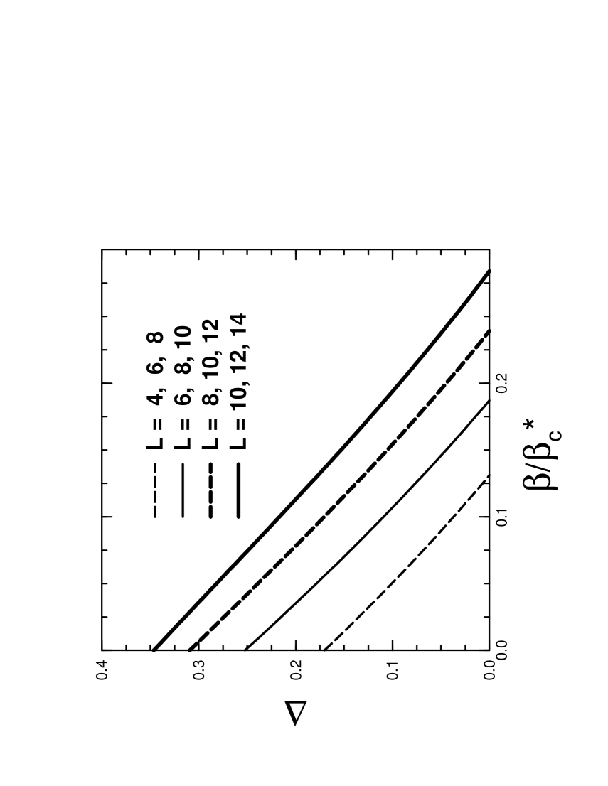
Figure 8: Extrapolated gap estimates $\Delta_{\{L\}}$ for the spin-1 Heisenberg chain with periodic boundary conditions.

Figure 9: We fit the CAM data to equation (27) while varying $Z$ in (26). The CAM data are equally weighted with an arbitrary fixed weight. The minimum of $\chi^{2}$ gives the best estimate for $\nu$.

Figure 10: CAM plot for the spin-1 Heisenberg chain. $Y$ and $X$ are give by (7) and (8), respectively. The solid curve is a fit to (27). The dashed line is the asymptote of the fitted curve.

References

- [1] Suzuki M 1995 Coherent Anomaly Method: Mean Field, Fluctuations and Systematics ed M Suzuki et al (Singapore: World Scientific)
- [2] Suzuki M 1995 Coherent Approaches to Fluctuations ed M Suzuki and N Kawashima (Singapore: World Scientific) pp 6–11
- [3] Suzuki M and Kolesik M 1996 Theory and Applications of the Cluster Variation and Path Probability Methods ed J L Morán-López and J M Sanchez (New York: Plenum) pp 113–124
- [4] Suzuki M 1986 J. Phys. Soc. Jpn. 55 4205–30
- [5] Onsager L 1944 Phys. Rev. 65 117–49
- [6] Fisher M E 1971 Proc. of the 51st Enrico Fermi Summer School ed M S Green (New York: Academic) pp 1–99
- [7] Fisher M E and Barber M N 1972 Phys. Rev. Lett. 28 1516–19
- [8] Barber M N 1983 Phase Transitions and Critical Phenomena vol 8 ed C Domb and J L Lebowitz (London: Academic) pp 145–266
- [9] Wegner F J 1972 Phys. Rev. B 5 4529–36
- [10] Burden R L and Faires J D 1989 Numerical Analysis (Boston: PSW-Kent) pp 146–154
- [11] Privman V and Fisher M E 1983 J. Phys. A 16 L295–L301
- [12] Baillie C F, Gupta R, Hawick K A and Pawley G S 1992 Phys. Rev. B 45 10438–53
- [13] Kolesik M and Suzuki M 1995 Physica A 215 138–51
- [14] Choi J-Y 1997 J. Phys. Soc. Jpn. 66 5–7
- [15] Novotny M A, Richards H L and Rikvold P A 1992 Mat. Res. Soc. Symp. Proc. vol 237 ed K S Liang et al (Pittsburgh: Materials Research Society) pp 67–72
- [16] Richards H L, Novotny M A and Rikvold P A 1993 Phys. Rev. B 48 14584–98
- [17] Nightingale M P and Blöte H W J 1996 Phys. Rev. B 54 1001–8
- [18] Burden R L and Faires J D 1989 Numerical Analysis (Boston: PSW-Kent) pp 68–71
- [19] Takhtajan L A 1982 Phys. Lett. 87 A 479–82
- [20] Babujian H M 1983 Phys. Lett. 90 A 479–82
- [21] Babujian H M 1983 Nucl. Phys. B 215 317–36
- [22] Affleck I, Kennedy T, Lieb E H and Tasaki H 1987 Phys. Rev. Lett. 59 799–802
- [23] Affleck I, Kennedy T, Lieb E H and Tasaki H 1988 Commun. Math. Phys. 115 477–528
- [24] Affleck I 1986 Nucl. Phys. B 216 409–47
- [25] Haldane F D M 1983 Phys. Rev. Lett. 50 1153–6
- [26] Haldane F D M 1983 Phys. Lett. 93A 464–8
- [27] Blöte H W J and Capel H W 1986 Physica A 139 387–94
- [28] Fáth G and Sólyom J 1993 Phys. Rev. B 47 872–81
- [29] White S R 1992 Phys. Rev. Lett. 69 2863–6
- [30] White S R 1993 Phys. Rev. B 48 10345–56
- [31] Kinosita Y, Kawashima N and Suzuki M 1992 J. Phys. Soc. Jpn. 61 3887–901
- [32] Östlund S and Rommer S 1995 Phys. Rev. Lett. 75 3537–40
- [33] Rommer S and Östlund S 1997 Phys. Rev. B 55 2164–81