Photon-Assisted Transport Through Ultrasmall Quantum Dots: Influence of Intradot Transitions

Abstract

We study transport through one or two ultrasmall quantum dots with discrete energy levels to which a time-dependent field is applied (e.g., microwaves). The AC field causes photon-assisted tunneling and also transitions between discrete energy levels of the dot. We treat the problem by introducing a generalization of the rotating-wave approximation to arbitrarily many levels. We calculate the dc-current through one dot and find satisfactory agreement with recent experiments by Oosterkamp et al. [Phys. Rev. Lett. 78, 1536 (1997)]. In addition, we propose a novel electron pump consisting of two serially coupled single-level quantum dots with a time-dependent interdot barrier.

I Introduction

Transport through small quantum dots has attracted considerable interest over the last couple of years. These quantum dots, small structures formed in a two-dimensional electron gas by applying appropriate gate voltages, are characterized by small capacitances to the substrate and to the leads connecting them to external voltage sources. Hence there is a sizeable charging energy $E_{C}=e^{2}/(2C)$ that has to be provided if electrons are to tunnel from the leads to the dot. Transport is blocked at small voltages, a phenomenon dubbed the Coulomb blockade since it is a direct consequence of the Coulomb interaction and the geometry of the dot. Another aspect that comes up for semiconductor quantum dots as opposed to small metallic islands is their discrete single-particle spectrum caused by size quantization.

Many aspects of the Coulomb blockade are now well understood. Recently, a new issue has come up, viz., time-dependent transport through small quantum dots. High-frequency AC voltages can be applied to mesoscopic structures (e.g., in the form of microwaves). They lead to photon-assisted tunneling, i.e., electrons can overcome the Coulomb blockade by absorbing photons from the external field. This has become a very active area recently both experimentally [2, 3, 4, 5, 1] and theoretically [6, 7, 8, 9, 10, 11].

In this work, we will study transport through an ultrasmall quantum dot with discrete energy levels to which a time-dependent field is applied. The electron interaction in the dots is taken into account by the Coulomb blockade model. The dots are weakly coupled to source and drain reservoirs by tunnel junctions. Time-dependent gate voltages lead to photon-assisted tunneling. In contrast to earlier theoretical work [6, 7, 8, 9, 10] we also take into account transitions between discrete energy levels of the dot. In addition, we propose a novel electron pump consisting of two serially coupled single-level quantum dots strongly coupled by time-dependent fields.

The paper is organized as follows: in Section II we introduce the Hamiltonian of a single interacting quantum dot with a time-dependent field, connected by tunnel junctions to source and drain reservoirs. We discuss the model and its solution by introducing a generalized version of the rotating-wave approximation (RWA). In the following section, we describe briefly the master equation technique we use to calculate the transport current. In this paper, the tunneling is always taken into account by performing a first-order perturbation expansion in the tunneling matrix element. This is equivalent to consider sequential tunneling, assuming the dot to be weakly coupled to the reservoirs such that higher-order tunneling processes can be neglected. In Section IV we describe the case of a dot with two discrete energy levels, which can be solved analytically. Our results for the current are presented in Section V and compared with recent experiments [1].

In Section VI we present a double-dot electron pump, which uses a time-dependent interdot barrier as the pumping mechanism. We use the Floquet-matrix technique to find a numerical solution to the problem, valid even in situations in which the RWA is not applicable.

II Model

As a model for an interacting quantum dot in a time-dependent periodic field coupled to two reservoirs by tunnel junctions we will use the time-dependent Hamiltonian $H(t)=H_{res}(t)+H_{dot}(t)+H_{tun}$[8]. Here

$$H_{res}(t)=\sum_{k,\alpha,\sigma}\epsilon^{\phantom{\dagger}}_{k\alpha\sigma}(t)\,c^{\dagger}_{k\alpha\sigma}c^{\phantom{\dagger}}_{k\alpha\sigma}$$ (1)

describes noninteracting electrons in the reservoirs $\{\alpha\}=\{L,R\}$, $c^{\dagger}_{k\alpha\sigma}/c^{\phantom{\dagger}}_{k\alpha\sigma}$ are the creation/annihilation operators of an electron with momentum $k$ and spin $\sigma$ in the reservoir $\alpha$. The energies $\epsilon^{\phantom{\dagger}}_{k\alpha\sigma}(t)=\epsilon^{0}_{k\alpha\sigma}+\Delta_{\alpha}\cos(\omega t)$ include a time-dependent shift of the Fermi energy of the electrons in the leads due to the applied periodic field, and $\Delta_{\alpha}$ denotes its coupling strength to the reservoir $\alpha$. The Hamiltonian for the interacting electrons in the dot is given by

$$H_{dot}(t)=\sum_{l,\sigma}\epsilon^{\phantom{\dagger}}_{l\sigma}(t)\,d^{\dagger}_{l\sigma}d^{\phantom{\dagger}}_{l\sigma}+\sum^{m<l}_{l,m,\sigma}w^{\phantom{\dagger}}_{lm}(t)\,d^{\dagger}_{l\sigma}d^{\phantom{\dagger}}_{m\sigma}+h.c.+H_{ch}(N_{dot})\;,$$ (2)

where $d^{\dagger}_{l\sigma}/d^{\phantom{\dagger}}_{l\sigma}$ create/annihilate electrons with spin $\sigma$ occupying level $l$ of the discrete, equidistant energy levels with level spacing $\Delta\epsilon$ in the dot ($l=1,2,...,N$ for a quantum dot with $N$ levels). The energy of level $l$ is given by $\epsilon^{\phantom{\dagger}}_{l\sigma}(t)=\epsilon^{0}_{l\sigma}+\Delta_{D}\cos(\omega t)$, where the time dependence is taken into account by a periodic shift of the level. The coupling strength of the field to the dot is given by $\Delta_{D}$. The time-dependent transition matrix elements $w^{\phantom{\dagger}}_{lm}(t)=\overline{\Delta}_{lm}\cos(\omega t)$ describe transitions from level $l$ to level $m$, i.e., transitions that do not change the number of electrons in the dot. The Coulomb interaction between electrons in the dot is taken into account by the Coulomb-blockade model

$$H_{ch}(N_{dot})=E_{C}N_{dot}^{2}\;.$$ (3)

Here, $N_{dot}=\sum_{l,\sigma}d^{\dagger}_{l\sigma}d^{\phantom{\dagger}}_{l\sigma}$ is the particle number in the dot, $E_{C}=e^{2}/2C$ is the charging energy with $C=C_{L}+C_{R}+C_{g}$. Note that we have already taken into account the time-dependent part $2N_{dot}\,n_{0}(t)$ of the original $H^{orig}_{ch}(N_{dot},t)=E_{C}[N_{dot}+n_{0}(t)]^{2}$ by the energies $\epsilon^{\phantom{\dagger}}_{l\sigma}(t)$ [8]. There $en_{0}(t)=C_{L}V_{L}(t)+C_{R}V_{R}(t)+C_{g}V_{g}(t)$ is related to the polarization charges produced by the time-dependent voltages of the left and right reservoirs $eV_{L/R}(t)=\mu_{L/R}+\Delta_{L/R}\cos(\omega t)$ as well as the time-dependent gate voltage $eV_{g}(t)=\mu_{g}+\Delta_{g}\cos(\omega t)$ applied to the quantum dot by the capacitance $C_{g}$. The tunneling part is given by

$$H_{tun}=\sum_{k,l,\alpha,\sigma}T^{\alpha}_{kl}\,c^{\dagger}_{k\alpha\sigma}d^{\phantom{\dagger}}_{l\sigma}+h.c.\;,$$ (4)

where $T^{\alpha}_{kl}$ denotes the tunneling matrix element.

The time-dependent Schrödinger equation ($\hbar=1$)

$$i{\partial\over\partial t}|\psi\rangle=H_{0}|\psi\rangle\qquad H_{0}(t)=H_{res}(t)+H_{dot}(t)$$ (5)

cannot be solved in a closed form due to the time-dependent off-diagonal matrix elements $w_{lm}(t)$ in Eq. (2). For

$$\Delta\epsilon\approx\omega\;,$$ (6)

one can approximate $w_{lm}(t)$ by

$$w^{\phantom{\dagger}}_{lm}(t)=\overline{\Delta}_{lm}\cos(\omega t)={\overline{\Delta}_{lm}\over 2}(e^{i\omega t}+e^{-i\omega t})\;\;\longrightarrow\;\;w^{\phantom{\dagger}}_{lm}(t)={\Delta_{lm}\over 2}e^{-i\omega(l-m)t}\;.$$ (7)

This is equivalent to omitting rapidly oscillating terms of frequency $\omega+\Delta\epsilon$, which is much larger than $\omega-\Delta\epsilon$ as long as (6) is fulfilled.

This can be understood as a generalization of the rotating-wave approximation, which is well-known in the theory of time-dependent two-level systems (e.g., in nuclear magnetic resonance [12] or quantum optics [13]). This generalization can be applied to systems with arbitrarily many levels. It makes it possible to perform a time-dependent unitary transformation $U(t)=U_{d}\,V(t)$ in Eq. (5) which removes the time dependence from the non-diagonal matrix elements of $H_{dot}$ [$V(t)$] and diagonalizes it afterwards [$U_{d}$]. Defining $|\widetilde{\psi}\rangle=U(t)|\psi\rangle$, the Schrödinger equation becomes

$$i{\partial\over\partial t}|\widetilde{\psi}\rangle=\widetilde{H}_{0}(t)|\widetilde{\psi}\rangle\qquad\widetilde{H}_{0}(t)=H_{res}+\widetilde{H}_{dot}(t)$$ (8)

with

$$\widetilde{H}_{dot}=UH_{dot}U^{\dagger}-iU({\partial\over\partial t}U^{\dagger})\;,$$ (9)

where $UH_{dot}U^{\dagger}=UH_{dot}^{\prime}U^{\dagger}+H_{ch}(N_{dot})$. The charging part of the Hamiltonian, $H_{ch}$, stays invariant under unitary transformations, since it depends only on the particle number on the dot. $H_{dot}^{\prime}$ is given by the following expression in matrix notation

$$H_{dot}^{\prime}(t)=\left(\begin{array}[]{cc}H^{\uparrow}_{dot}(t)&0\\ 0&H^{\downarrow}_{dot}(t)\end{array}\right)\;,$$ (10)

where the submatrices $H^{\sigma}_{dot}$ with spin index $\sigma=\{\uparrow,\downarrow\}$ are given by

$$H^{\sigma}_{dot}(t)={1\over 2}\left(\begin{array}[]{ccccc}2\epsilon^{\phantom{\dagger}}_{1\sigma}(t)&\Delta^{*}_{1}e^{i\omega t}&\Delta^{*}_{2}e^{i2\omega}&\cdots&\Delta^{*}_{N-1}e^{i(N-1)\omega}\\ \Delta_{1}e^{-i\omega t}&2\epsilon^{\phantom{\dagger}}_{2\sigma}(t)&\Delta^{*}_{1}e^{i\omega t}&\cdots&\Delta^{*}_{N-2}e^{i(N-2)\omega}\\ \Delta_{2}e^{-i2\omega t}&\Delta_{1}e^{-i\omega t}&2\epsilon^{\phantom{\dagger}}_{3\sigma}(t)&\cdots&\Delta^{*}_{N-3}e^{i(N-3)\omega}\\ \vdots&\vdots&\vdots&\ddots&\vdots\\ \Delta_{N-1}e^{-i(N-1)\omega t}&\Delta_{N-2}e^{-i(N-2)\omega t}&\Delta_{N-3}e^{-i(N-3)\omega t}&\cdots&2\epsilon^{\phantom{\dagger}}_{N\sigma}(t)\end{array}\right)\;.$$ (11)

Here we have assumed $\Delta_{lm}=\Delta_{|l-m|}$ for simplicity. Then $V(t)$ is

$$V(t)=\left(\begin{array}[]{cc}V^{\uparrow}(t)&0\\ 0&V^{\downarrow}(t)\end{array}\right)$$ (12)

$$V^{\sigma}(t)=\left(\begin{array}[]{ccccc}e^{-i\omega t/2}&0&0&\cdots&0\\ 0&e^{i\omega t/2}&0&\cdots&0\\ 0&0&e^{i3\omega t/2}&\cdots&0\\ \vdots&\vdots&\vdots&\ddots&\vdots\\ 0&0&0&\cdots&e^{i(2N-3)\omega t/2}\end{array}\right)\;.$$ (13)

The eigenenergies $\widetilde{\epsilon}^{0}_{j\sigma}$ ($j=1,2,...,N$) of $\widetilde{H}_{dot}(t)$ are then obtained by numerical diagonalization. The transformed tunneling part of the Hamiltonian is given by

$$\widetilde{H}_{tun}(t)=\sum_{k,j,\alpha,\sigma}\widetilde{T}^{\alpha}_{kj}(t)\,c^{\dagger}_{k\alpha\sigma}\widetilde{d}^{\phantom{\dagger}}_{j\sigma}+h.c.\;,$$ (14)

where $\widetilde{d}^{\dagger}_{j\sigma}/\widetilde{d}^{\phantom{\dagger}}_{j\sigma}$ are the creation/annihilation operators of an electron with spin $\sigma$ that occupies the level with energy $\widetilde{\epsilon}^{0}_{j\sigma}$, and

$$\widetilde{T}^{\alpha}_{kj}(t)=\sum_{l}{(U_{d})}^{*}_{jl}\,T^{\alpha}_{kl}\,e^{-i(2l-3)\omega t/2}\;.$$ (15)

In addition, for a dot with only two levels the diagonalization can also be performed analytically, providing further insight in the underlying physics (see below in Section IV).

III The master-equation approach

$\widetilde{H}_{dot}(t)$ generates the time-evolution operator $U_{0}(t,t_{0})=\exp(-i\int_{t_{0}}^{t}d\tau\widetilde{H}_{0}(\tau))$, which is needed to calculate the tunneling Hamiltonian $\widetilde{H}^{I\alpha}_{tun}(t)=U_{0}(t_{0},t)\widetilde{H}^{\alpha}_{tun}(t)U_{0}(t,t_{0})$ in the interaction representation.

The von Neumann-equation $i\dot{\varrho}(t)=[\widetilde{H}_{0}(t)+\widetilde{H}_{tun}(t),\varrho(t)]$ that describes the time evolution of the density matrix is also transformed to the interaction representation and $\varrho$ is expanded to first order in the tunneling rate. This leads to a master equation for the occupation probabilities [8] $P_{s}(t)=\langle s|\varrho(t)|s\rangle$ of the occupation number states $|s\rangle$. The states $|s\rangle$ represent the occupation numbers of the energy levels of the diagonalized system. In the time-averaged dc-case the master equation can be written as a system of coupled linear equations

$$\sum_{s^{\prime}}[\Gamma_{s^{\prime}\rightarrow s}-\delta_{ss^{\prime}}(\sum_{s^{\prime\prime}}\Gamma_{s^{\prime}\rightarrow s^{\prime\prime}})]P_{s^{\prime}}=0\;,$$ (16)

which can be solved approximately by a suitable truncation. The rate $\Gamma_{s^{\prime}\rightarrow s}$ for a transition from state $|s^{\prime}\rangle$ to $|s\rangle$ can be expressed as $\Gamma_{s^{\prime}\rightarrow s}=\Gamma^{L}_{s^{\prime}\rightarrow s}+\Gamma^{R}_{s^{\prime}\rightarrow s}$, where

$$\Gamma^{\alpha}_{s^{\prime}\rightarrow s}={\omega\over\pi}\int^{2\pi/\omega}_{0}dt\int^{\infty}_{0}d\tau\;Re\{\,\langle s|\widetilde{H}^{I\alpha}_{tun}(t)|s^{\prime}\rangle\langle s^{\prime}|\widetilde{H}^{I\alpha}_{tun}(t-\tau)|s\rangle\,\}$$ (17)

is the rate associated with tunneling processes from/to reservoir $\alpha$. $\widetilde{H}^{I\alpha}_{tun}(t)$ denotes the part of the tunneling Hamiltonian (14) in the interaction picture that corresponds to that reservoir.

The dc-current through the junction connecting the dot with reservoir $\alpha$ now can be expressed in terms of the occupation probabilities and transition rates as well as $N_{dot}(s)$ (the particle number on the dot while being in state $|s\rangle$) as

$$I^{\alpha}_{dc}=-e\sum_{s,s^{\prime}}\Gamma^{\alpha}_{s^{\prime}\rightarrow s}[N_{dot}(s^{\prime})-N_{dot}(s)]\,P_{s}^{\prime}\;.$$ (18)

By this means it is possible to numerically calculate the current as a function of transport or gate voltage. However, to really understand the resulting I-V-curves, it is helpful to have a closer look at the analytically solvable case with only two energy levels in the dot.

IV Two-level case

The matrix (11) reduces to

$$H^{\sigma}_{dot}={1\over 2}\left(\begin{array}[]{cc}2\epsilon^{\phantom{\dagger}}_{1\sigma}(t)&\Delta^{*}e^{i\omega t}\\ \Delta e^{-i\omega t}&2\epsilon^{\phantom{\dagger}}_{2\sigma}(t)\end{array}\right)$$ (19)

with $\epsilon^{\phantom{\dagger}}_{l\sigma}(t)=\epsilon^{0}_{l\sigma}+\Delta_{D}\cos(\omega t)$. The transformation that renders the non-diagonal elements time-independent is given by

$$V^{\sigma}(t)=\left(\begin{array}[]{cc}e^{-i\omega t/2}&0\\ 0&e^{i\omega t/2}\end{array}\right)\;.$$ (20)

Applying $U(t)$ to the Schrödinger equation leads to

$$\widetilde{H}_{dot}={1\over 2}U^{\phantom{\dagger}}_{d}\left(\begin{array}[]{cccc}2\epsilon^{\phantom{\dagger}}_{1\uparrow}(t)+\omega&\Delta^{*}&0&0\\ \Delta&2\epsilon^{\phantom{\dagger}}_{2\uparrow}(t)-\omega&0&0\\ 0&0&2\epsilon^{\phantom{\dagger}}_{1\downarrow}(t)+\omega&\Delta^{*}\\ 0&0&\Delta&2\epsilon^{\phantom{\dagger}}_{2\downarrow}(t)-\omega\\ \end{array}\right)U^{\dagger}_{d}\;.$$ (21)

Calculating $U_{d}$ and the new energies $\widetilde{\epsilon}_{j\sigma}(t)$ is now straightforward, they are given by

$$\widetilde{\epsilon}_{j\sigma}(t)={(\epsilon^{0}_{1\sigma}+\epsilon^{0}_{2\sigma})\over 2}+{(-1)}^{j}{\Omega\over 2}+\Delta_{D}\cos(\omega t)\;,$$ (22)

where $\Omega=\sqrt{(\Delta\epsilon-\omega)^{2}+|\Delta|^{2}}$ is the Rabi frequency and $\Delta\epsilon=\epsilon^{0}_{2\sigma}-\epsilon^{0}_{1\sigma}$. After calculating $U_{d}$ we can write down the creation/annihilation operators $\widetilde{d}^{\dagger}_{j\sigma}/\widetilde{d}^{\phantom{\dagger}}_{j\sigma}$ for an electron that occupies energy level $j$ ($j=1,2$) as well as the corresponding time-dependent tunneling matrix elements $\widetilde{T}^{\alpha}_{kj}(t)$. Defining the quantity $\hat{\epsilon}=\Delta\epsilon-\omega\pm\Omega$ for $\omega{\phantom{|}}^{<}_{>}{\phantom{|}}\Delta\epsilon$, these matrix elements are

$$\widetilde{T}^{\alpha}_{k1}(t)={1\over\sqrt{\hat{\epsilon}^{2}+|\Delta|^{2}}}\,[T^{\alpha}_{k1}\,\hat{\epsilon}\,e^{i\omega t/2}-T^{\alpha}_{k2}\,\Delta\,e^{-i\omega t/2}]$$ (23)

$$\widetilde{T}^{\alpha}_{k2}(t)={1\over\sqrt{\hat{\epsilon}^{2}+|\Delta|^{2}}}\,[T^{\alpha}_{k2}\,\hat{\epsilon}\,e^{-i\omega t/2}+T^{\alpha}_{k1}\,\Delta^{*}\,e^{i\omega t/2}]\;.$$ (24)

Writing down the tunneling Hamiltonian with these matrix elements and creation/annihilation operators and inserting them into the master equation then permits us to calculate the current in a straightforward way. It turns out that there are two possible ways for an electron to tunnel through the dot, corresponding to the two terms with $e^{\pm i\omega t/2}$ in the tunneling matrix elements (Fig. 1). The transport peaks present in the absence of a time-dependent field are split in a two-peak group (with peaks at distance $\omega$) that also shifts its position due to the $\Delta$-dependence of the energies $\widetilde{\epsilon}_{j\sigma}(t)$.

V Results

For a dot with two spin-degenerate levels four groups of current peaks will appear in the I-V-curve, separated from each other by $2E_{C}$. If the field-induced inner transitions between the levels are neglected (all $\Delta_{|l-m|}=0$), there is one main peak per group accompanied by Bessel-type sidebands at separations $n\omega$ (with $n=\pm 1,\pm 2,\pm 3,...$). These side peaks are due to photon-assisted tunneling (PAT) [8]. The existence of these side peaks has been recently verified experimentally [1].

If inner transitions are taken into account, our calculations show that the single main peak will shift with increasing $\Delta_{|l-m|}$. In addition, $N-1$ peaks will appear at distances $n\omega$ (with $n=1,...,N-1$), see also Fig. 1. This leads to a totally different picture of the current-peak positions and heights, the weight of the peaks shifts as well as their positions.

To visualize only the influence of inner transitions, we set $\Delta_{D}=0$, i.e, there is no PAT, and plot the peak group corresponding to a dot occupied by one additional electron as a function of the increasing strength of the inner transitions (increasing $\Delta_{|l-m|}$). Two cases, one with two and one with three degenerate energy levels are shown (Fig. 3). The shift of the main peak and the appearance of the one (two) additional peak(s) as described above is clearly visible.

Of course it is also possible to include the inner transitions in the master equation in a perturbative way. To do this, transition rates between the levels (similar to those describing the tunneling of electrons to and from the dot) have to be calculated in first-order perturbation theory. Then the peaks do not shift with increasing $\Delta_{|l-m|}$, because the master equation is written in the basis of the unperturbed states. But also the effect on the peak heights is significantly smaller than in our modified rotating-wave approximation approach. In Fig. 2 this is illustrated by plotting again the peak group for a dot with two levels and one extra electron. Again we set $\Delta_{D}=0$, i.e., neglecting PAT. For a fixed, relatively small value of $\Delta$, the peak shift is not significant.

In recent transport measurements on ultrasmall quantum dots with applied microwaves such a peak group was studied [1]. A dot with two levels contributing to transport was used. The first side peak rises more strongly with increasing microwave power than expected from the PAT model. In Fig. 4 we compare the measured I-V-curves with our results. For small values of $\Delta$ our model is in good agreement with the experiment for both microwave frequencies. In particular it describes correctly the strong increase of the right side peak. The numerical calculations have been done using non-degenerate levels because in the experiments a strong magnetic field ($B=0.91T$) (which was supposed to suppress plasmon excitations) lifted the spin degeneracy.

VI Double quantum-dot electron pump: Floquet-matrix approach

The single quantum dot with two discrete energy levels connected by a matrix element $w_{lm}(t)=\Delta_{0}+\Delta\cos(\omega t)$ can be mapped to a double dot system where two dots with one energy level are strongly coupled with each other. But in the formalism discussed above it would not be possible in this case to choose the gate voltages and the microwave frequency arbitrarily, due to the restrictions imposed by the rotating-wave approximation. Also, the time-dependence of the two gate voltages would have to be the same for both dots.

In this section we discuss a double dot system with time-dependent gate voltages that differ by a relative phase $\varphi$. The dots are strongly coupled by a time-dependent tunneling barrier . Such a system connected to reservoirs as shown in Fig. 5 can work as a electron pump, resulting in a current even if no transport voltage is applied. We generalize the work of Stafford and Wingreen[10] to the case where the height of the tunneling barrier also depends on time. The time-dependent Schrödinger equation is solved by the Floquet-matrix approach[14]. In general, according to Floquet’s theorem, a differential equation with periodic coefficients like equation (5) has solutions of the form (for a dot with $N$ levels) [15]

$$|\psi_{j}(t)\rangle=e^{-i\tilde{\epsilon}_{j}t}\,|\varphi_{j}(t)\rangle\;\;\;(j=1,...,N)\;,$$ (25)

which inserted in the Schrödinger equation (5) result in an eigenvalue problem for the states $|\varphi_{j}\rangle$

$$(H(t)-i{\partial\over\partial t})\,|\varphi_{j}\rangle=\widetilde{\epsilon}_{j}|\varphi_{j}\rangle\;.$$ (26)

The states $|\varphi_{j}\rangle$ have the same periodicity as the dot Hamiltonian, i.e., $|\varphi_{j}(t+2\pi/\omega)\rangle=|\varphi_{j}(t)\rangle$. Due to this it is possible to expand $H_{dot}(t)$ and $|\varphi_{j}(t)\rangle$ in a Fourier series

$$H_{dot}(t)=\sum_{n=-\infty}^{\infty}H_{dot}^{(n)}e^{in\omega t}$$ (27)

$$|\varphi_{j}(t)\rangle=\sum_{n=-\infty}^{\infty}e^{in\omega t}|\varphi^{(n)}_{j}\rangle\;.$$ (28)

In the basis $\{|\,l\,\rangle\}$ of the eigenstates of the diagonal dot Hamiltonian $H^{0}_{dot}=\sum_{l,\sigma}\epsilon^{0}_{l}d^{\dagger}_{l\sigma}d^{\phantom{\dagger}}_{l\sigma}$ with uncoupled energy levels $\epsilon^{0}_{l}$ (i.e., $H^{0}_{dot}|\,l\,\rangle=\epsilon^{0}_{l}|\,l\,\rangle$), the solution $|\psi_{j}(t)\rangle$ can be expressed as

$$|\psi_{j}(t)\rangle=\sum_{l=1}^{N}\langle\,l\,|\varphi_{j}(t)\rangle\,e^{-i\tilde{\epsilon}_{j}t}\,|\,l\,\rangle=\sum_{l=1}^{N}\sum_{n=-\infty}^{\infty}e^{-i\tilde{\epsilon}_{j}t}e^{in\omega t}\,\varphi^{(n)}_{lj}\,|\,l\,\rangle\;.$$ (29)

If we insert (27) and (29) in the time-dependent Schrödinger equation (5), multiply with the bra $\langle\,i\,|$ from the left and define the matrix elements $H^{(n)}_{il}=\langle\,i\,|H_{dot}^{(n)}|\,l\,\rangle$, we get an infinite system of coupled linear equations describing the eigenvalue problem for the quasi-energies $\tilde{\epsilon}_{j}$

$$\sum_{l=1}^{N}\sum_{k=-\infty}^{\infty}\,[H^{(n-k)}_{il}+n\omega\delta_{nk}\delta_{il}]\,\varphi^{(k)}_{lj}=\tilde{\epsilon}_{j}\varphi^{(n)}_{ij}\;.$$ (30)

If $H_{dot}(t)$ is given by (2) with $w_{lm}(t)={\Delta_{0}}_{\,lm}+\Delta_{lm}\cos(\omega t)$, this becomes

$$\sum_{l=1}^{N}\sum_{k=-\infty}^{\infty}\,[((\epsilon^{0}_{l}+n\omega)\delta_{il}+{\Delta_{0}}_{il})\delta_{nk}+{\Delta_{il}\over 2}(\delta_{n,k+1}+\delta_{n,k-1})]\,\varphi^{(k)}_{lj}=\tilde{\epsilon}_{j}\varphi^{(n)}_{ij}\;.$$ (31)

The quasi-energies $\tilde{\epsilon}_{j}$ and the eigenvector components $\varphi^{(n)}_{ij}$ can be calculated numerically by truncating this infinite system of coupled equations at a sufficiently large finite $n$. It is now possible to transform the tunneling Hamiltonian and calculate the current by the master equation technique analogous to the previous sections. The resulting dependence of the pumped current on the frequency and the amplitude of the applied microwaves is plotted in Fig. 6 and Fig. 7. Here and in the rest of the paper we used $E_{ch}=75\Gamma$,$\;\Gamma_{L}=\Gamma_{R}=\Gamma$. In Fig. 6 and Fig. 7 we set $\epsilon_{1}=-10\Gamma$,$\;\epsilon_{2}=10\Gamma$,$\;\mu_{L}=\mu_{R}=0$, $\;T=5\Gamma$.

Figure 6 illustrates the situation where the microwaves couple only to the interdot barrier. There are current peaks if the photon energy equals an integer fraction of the quasi-energy level splitting. Because the quasi-energies themselves depend on the amplitude $\Delta$ (analogous to the RWA calculations above), the current peaks shift to higher photon energies with increasing $\Delta$. This plot illustrates the effect created purely by a time-dependent barrier.

However, in a real experiment the microwaves would also couple to the gate electrodes and the interdot coupling would have a finite time-independent part, i.e., $w_{lm}(t)=\Delta_{0}+\Delta\cos(\omega t)$. This is shown in Fig. 7. It is clearly seen that the overall peak height increases compared to Fig. 6.

The behavior of the current through an interacting double quantum dot for finite transport voltages and two independently varied gate voltages is plotted in Fig. 8 and Fig. 9 ($\mu_{L}=2.5\Gamma$,$\;\mu_{R}=-2.5\Gamma$,$\;T=3\Gamma$ in both figures). Figure 8 illustrates the case where the microwaves are coupled to the interdot barrier only, i.e., with a time-dependent coupling matrix element. Instead, in Fig. 9 the microwaves are coupled to the gate electrodes, assuming a static interdot matrix element. As can be clearly seen, the same value for the coupling matrix element in both case leads to a significant increase of $I_{max}$.

In conclusion, we have calculated the photon-assisted transport current through a single interacting quantum dot with an arbitrary number of discrete energy levels. We have taken into account field-induced inner transitions in a non-perturbative way by generalizing the rotating-wave approximation to more then two energy levels. We compare our results to recent experiments [1] and provide an explanation for the unexpected height of the first side-band current peak.

We would like to thank J. König and G. Schön for discussions and suggestions and especially T. H. Oosterkamp and L. P. Kouwenhoven for providing us with the experimental data. The support by the Deutsche Forschungsgemeinschaft, through SFB 195, is gratefully acknowledged.

FIG. 1.: Energy landscape of a quantum dot with two non-degenerate levels and inner transitions induced by a time-dependent field of frequency $\omega$. The effective energy levels $\widetilde{\epsilon}_{j}$ are shown (solid lines). Note that electron transport occurs, when the chemical potentials $\mu_{L/R}$ match one of the quasi-levels (dashed lines) shifted from the energies $\widetilde{\epsilon}_{j}$ by $\pm\omega/2$ due to the time-dependent tunneling matrix elements $\widetilde{T}^{\alpha}_{kj}(t)$.

FIG. 2.: $I_{dc}$-$V_{g}$-curve for a dot with two degenerate levels. The RWA model (solid curve) is compared with first-order perturbation theory for calculating the transition rates between the two energy levels (dashed curve). In RWA the first side peak is significantly enhanced. $\epsilon_{1}=-25\Gamma$, $\epsilon_{2}=25\Gamma$, $\omega=60\Gamma$, $T=5\Gamma$, $\Gamma_{1}=\Gamma_{2}=0.5\Gamma$, $\Delta_{D}=0$, $\Delta=10\Gamma$.

FIG. 3.: Evolution of the current-peak group corresponding to one electron occupying a dot with two (top) and three (bottom) spin-degenerate levels with increasing $\Delta$. PAT has been omitted. $\Delta_{D}=0$,$\;\Delta\epsilon=95\Gamma$,$\;\omega=55\Gamma$,$\;T=3\Gamma$.

FIG. 4.: Measured $I_{dc}$-$V_{g}$-curves (solid lines) (Oosterkamp et al.[1]) with applied microwaves of frequencies $42\,$GHz (left column) and $61.45\,$GHz (right column) versus our theoretical results (dashed lines). Left column: $\Gamma_{1}=0.2\Gamma$, $\Delta_{D}=1.875\Delta$. Right column: $\Gamma_{1}=0.1\Gamma$, $\Delta_{D}=3.5\Delta$. In both cases, $\Delta_{L}=-{1\over 170}\Delta_{D}$, $\Delta_{R}=-{1\over 220}\Delta_{D}$. Parameters determined by the experiment: $\epsilon_{1}=-47.5\Gamma$, $\epsilon_{2}=47.5\Gamma$, $\omega=135\Gamma$ (left), $\omega=200\Gamma$ (right), and $\Gamma=1.287\mu$eV.

FIG. 5.: Energy landscape of two serially coupled quantum dots connected by a weak time-dependent barrier (periodicity $\omega$). A additional time dependence may also be applied to the gate electrodes of both dots. With $\mu_{L}=\mu_{R}$ and applied microwaves the system works as an electron pump, pumping electrons “uphill” from left to right.

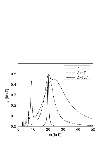
FIG. 6.: Current response of a double quantum-dot electron pump versus frequency $\omega$ for a time-dependent barrier separating the dots. $\Delta_{0}=0$, $\;\Delta_{D}=0$.

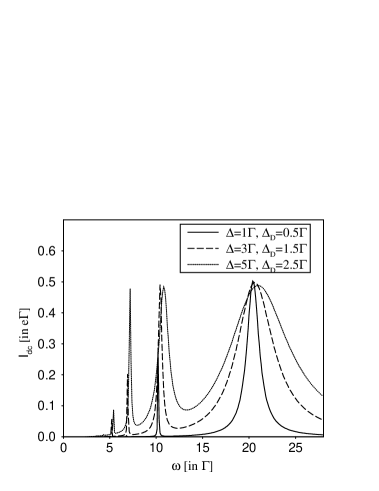
FIG. 7.: Same as Fig. 6 with time-dependent gate voltages and assuming a phase difference of $\pi$ between the two gates. $\Delta_{0}=2\Gamma$.

FIG. 8.: Dependence of the transport current on the positions of the energy levels, i.e., the gate voltages, for a time-dependent interdot barrier. $\Delta_{0}=2\Gamma$,$\;\Delta=3\Gamma$,$\;\Delta_{D}=0$.

FIG. 9.: Same as Fig. 8 for static interdot coupling ($\Delta=0$) and time-dependent gate voltages, assuming a phase difference of $\pi$ between the two gates. $\Delta_{0}=2\Gamma$,$\;\Delta=0$,$\;\Delta_{D}=3\Gamma$.

REFERENCES

- [1] T. H. Oosterkamp, L. P. Kouwenhoven, A. E. A. Koolen, N. C. van der Vaart, and C. J. P. M. Harmans, Phys. Rev. Lett. 78, 1536 (1997).
- [2] L. P. Kouwenhoven, S. Jauhar, K. McCormick, D. Dixon, P. L. McEuen, Y. V. Nazarov, N. C. van der Vaart, and C. T. Foxon, Phys. Rev. B 50, 2019 (1994).
- [3] L. P. Kouwenhoven, S. Jauhar, J. Orenstein, P. L. McEuen, Y. Nagamune, J. Motohisa, and H. Sakaki, Phys. Rev. Lett. 73, 3443 (1994).
- [4] R. H. Blick, R. J. Haug, D. W. van der Weide, K. von Klitzing, and K. Ebert, Appl. Phys. Lett. 67, 3924 (1995); R. H. Blick, R. J. Haug, K. von Klitzing, and K. Ebert, Surf. Science 361 595 (1996).
- [5] K. Fujii, W. Goedel, D. A. Wharam, S. Manus, J. P. Kotthaus, G. Böhm, W. Klein, G. Tränkle, and G. Weimann, Physica B 227, 98 (1996).
- [6] M. Büttiker, A. Prêtre, and H. Thomas, Phys. Rev. Lett. 70, 4114 (1993).
- [7] N. S. Wingreen, A. Jauho, and Y. Meir, Phys. Rev. B 48, 8487 (1993); A.Jauho, N. S. Wingreen, and Y. Meir, Phys. Rev. B 50, 5528 (1994).
- [8] C. Bruder and H. Schoeller, Phys. Rev. Lett. 72, 1076 (1994); C. Bruder and H. Schoeller, in Quantum Dynamics of Submicron Structures, edited by H. A. Cerdeira, B. Kramer, and G. Schön, NATO ASI Ser. E, Vol. 291 (Kluwer, Dordrecht, 1995), p. 383.
- [9] T. H. Stoof and Y. V. Nazarov, Phys. Rev. B 53, 1050 (1996).
- [10] C. A. Stafford and N. S. Wingreen, Phys. Rev. Lett. 76, 1916 (1996).
- [11] Y. Isawa, A. Okamoto, and T. Hatano, preprint.
- [12] F. Bloch and A. Siegert, Phys. Rev. 57, 522 (1940).
- [13] E. T. Jaynes and F. W. Cummings, IEEE Proc. 51, 89 (1963).
- [14] J. H. Shirley, Phys. Rev. 138, B979 (1965).
- [15] M. Holthaus and D. Hone, Phys. Rev. B 47, 6499 (1993).