An Exactly Solvable Model of $N$ Coupled Luttinger Chains

Abstract

We calculate the exact Green function of a special model of $N$ coupled Luttinger chains with arbitrary interchain hopping $t_{\perp}$. The model is exactly solvable via bosonization if the interchain interaction does not fall off in the direction perpendicular to the chains. For any finite $N$ we find Luttinger liquid behavior and explicitly calculate the anomalous dimension $\gamma^{(N)}$. However, the Luttinger liquid state does not preclude coherent interchain hopping. We also show that $\gamma^{(N)}\to 0$ for $N\to\infty$, so that in the limit of infinitely many chains we obtain a Fermi liquid.

The normal metallic state of interacting electrons in one spatial dimension is called a Luttinger liquid, and has fundamentally different properties than the Fermi liquid state in higher-dimensional Fermi systems. In particular, the single-particle Green function of a Luttinger liquid does not have a quasi-particle peak, but exhibits spin-charge separation and anomalous scaling properties. In order to calculate the physical properties of Luttinger liquids, non-perturbative methods are necessary, such as the bosonization method [1]. Recently the crossover from Luttinger liquid to Fermi liquid behavior as function of some suitable parameter has received much attention [2], partially because of Anderson’s and coworkers’ suggestion that higher-dimensional Luttinger liquid behavior might be the key to understand high-temperature superconductivity. An experimentally important class of systems exhibiting the above mentioned crossover are quasi-one-dimensional chain-like metals. In the normal metallic state (which is realized at sufficiently high temperatures), these systems can be described as one-dimensional Luttinger liquids that are coupled by small interchain hopping $t_{\bot}$ and by the three dimensional interaction. While for $t_{\bot}=0$ the number of particles on each chain is conserved and the problem can be studied in a straightforward way via bosonization, the case of $t_{\bot}\neq 0$ is more difficult and has recently been studied by means of a variety of non-perturbative methods. Most authors have focused on the crossover as a function of the dimensionless parameter $t_{\bot}/E_{F}$ (where $E_{F}$ is the Fermi energy), assuming that this parameter is small. In this work we shall show that for some special type of interactions (see below) it is possible to obtain an exact solution for the Green function of an arbitrary number of coupled Luttinger chains with finite $t_{\bot}$. The interaction is characterized by the fact that it does not fall off in the transverse direction. Although such an interaction is unphysical, our model is useful for testing the various approximations employed in the literature.

Let us start with a two-dimensional system of interacting fermions moving on an array of $N$ weakly coupled spin $1/2$ chains in the $x$-direction. Each chain can be described by the Tomonaga-Luttinger model with spin [3]. Denoting by $k_{\|}$ the momentum along the chains and linearizing the energy dispersion in the chain direction, the kinetic energy part of the Hamiltonian can be written as

$$H_{\rm kin}=\sum_{i,j}\sum_{\alpha,\sigma}\sum_{k_{\parallel}}\left[\delta_{i,j}\epsilon^{\alpha}(k_{\parallel})-t_{ij}\right]\left(\hat{c}_{i\sigma}^{\alpha{\dagger}}(k_{\parallel})\hat{c}_{j\sigma}^{\alpha}(k_{\parallel})-\langle\hat{c}_{i\sigma}^{\alpha{\dagger}}(k_{\parallel})\hat{c}_{j\sigma}^{\alpha}(k_{\parallel})\rangle_{0}\right)\;\;\;,$$ (1)

where $\hat{c}_{i\sigma}^{\alpha{\dagger}}(k_{\parallel})$ and $\hat{c}_{i\sigma}^{\alpha}(k_{\parallel})$ are the creation and annihilation operators for the right and left moving fermions $(\alpha=+,-)$ on chain $i=[-\frac{N}{2}+1],\ldots,[\frac{N}{2}]$ with spin $\sigma=\uparrow,\downarrow$ and momentum $k_{\parallel}$ in the chain direction. The linearized energy dispersions are $\epsilon^{\pm}(k_{\parallel})=v_{F}(\pm k-k_{F})$, where $v_{F}$ is the Fermi velocity and $k_{F}$ is the Fermi momentum associated in the absence of interchain hopping. For simplicity we assume only nearest neighbor hopping and impose periodic boundary conditions in the transverse direction. In this case the interchain hopping is for $N>2$ of the form $t_{ij}=t_{i-j,0}=\delta_{|i-j|,1}t_{\perp}/2$. In the special case of just two chains periodic boundary conditions are automatically satisfied and we set $t_{ij}=t_{\perp}\delta_{|i-j|,1}$. Because of the discrete translational invariance in the transverse direction (the $y$-direction) we can completely diagonalize $H_{\rm kin}$ via a discrete Fourier transformation in the transverse direction. Denoting by $k_{\perp}$ the corresponding transverse momentum and defining $\hat{c}_{\sigma}^{\alpha}({\bf k})=N^{-1/2}\sum_{i}e^{-ik_{\perp}y_{i}}\hat{c}_{i\sigma}^{\alpha}(k_{\parallel})$, we have

$$H_{\rm kin}=\sum_{\alpha,\sigma}\sum_{{\bf k}}\epsilon^{\alpha}({\bf k})\left[\hat{c}_{\sigma}^{\alpha{\dagger}}({\bf k})\hat{c}_{\sigma}^{\alpha}({\bf k})-\langle\hat{c}_{\sigma}^{\alpha{\dagger}}({\bf k})\hat{c}_{\sigma}^{\alpha}({\bf k})\rangle_{0}\right]\;\;\;,$$ (2)

where ${\bf k}=(k_{\parallel},k_{\perp})$, and the ${\bf k}$-dependent energy dispersion is given by $\epsilon^{\alpha}({\bf k})=\epsilon^{\alpha}(k_{\parallel})-t(k_{\perp})$, with $t(k_{\perp})=t_{\perp}\cos(k_{\perp}a_{\perp})$. Here $a_{\bot}$ is the distance between the chains. The corresponding Fermi surface is shown in Fig.1.

The total Hamiltonian is given by $H=H_{\rm kin}+H_{\rm int}$, where the interaction part is in general of the form

$$H_{\rm int}=\frac{1}{2}\frac{1}{2L}\sum_{i,j}\sum_{\alpha,\alpha^{\prime}}\sum_{\sigma,\sigma^{\prime}}\sum_{q_{\parallel}}f_{ij\sigma\sigma^{\prime}}^{\alpha\alpha^{\prime}}(q_{\parallel}):\hat{\rho}_{i\sigma}^{\alpha{\dagger}}(q_{\parallel})\hat{\rho}_{j\sigma^{\prime}}^{\alpha^{\prime}}(q_{\parallel}):\quad.$$ (3)

Here, one factor of $1/2$ has been introduced for convenience due to the spin, and the Fourier components of the density operators associated with chain $i$ are given by

$$\hat{\rho}^{\alpha}_{i\sigma}(q)=\sum_{k}\left(\hat{c}^{\alpha{\dagger}}_{i\sigma}(k)\hat{c}^{\alpha}_{i\sigma}(k+q)-\left<\hat{c}^{\alpha{\dagger}}_{i\sigma}(k)\hat{c}^{\alpha}_{i\sigma}(k+q)\right>_{0}\right)\;\;\;.$$ (4)

Assuming spin and inversion symmetry, we thus assume that the interaction parameters satisfy $f^{++}_{\sigma\sigma^{\prime}}=f^{--}_{\sigma\sigma^{\prime}}$, $f^{+-}_{\sigma\sigma^{\prime}}=f^{-+}_{\sigma\sigma^{\prime}}$, $f_{\parallel}^{\alpha\alpha^{\prime}}\equiv f_{\uparrow\uparrow}^{\alpha\alpha^{\prime}}=f_{\downarrow\downarrow}^{\alpha\alpha^{\prime}}$, and $f_{\perp}^{\alpha\alpha^{\prime}}\equiv f_{\uparrow\downarrow}^{\alpha\alpha^{\prime}}=f_{\downarrow\uparrow}^{\alpha\alpha^{\prime}}$. Performing the complete Fourier transformation of $H_{\rm int}$ by defining

$$\hat{\rho}_{\sigma}^{\alpha}({\bf q}) = \frac{1}{\sqrt{N}}\sum_{{\bf k}}\Big{(}\hat{c}_{\sigma}^{\alpha{\dagger}}({\bf k})\hat{c}_{\sigma}^{\alpha}({\bf k}+{\bf q})-\langle\hat{c}_{\sigma}^{\alpha{\dagger}}({\bf k})\hat{c}_{\sigma}^{\alpha}({\bf k}+{\bf q})\rangle_{0}\Big{)}\;\;\;,$$ (5)

$$f_{\sigma\sigma^{\prime}}^{\alpha\alpha^{\prime}}({\bf q}) = \sum_{i}e^{-iq_{\perp}y_{i}}f_{i0\sigma\sigma^{\prime}}^{\alpha\alpha^{\prime}}(q_{\parallel})\;\;\;,$$ (6)

and going over to a charge/spin basis,

$$\hat{\rho}_{c/s}^{\alpha}({\bf q}) = \frac{1}{\sqrt{2}}\left[\hat{\rho}_{\uparrow}^{\alpha}({\bf q})\pm\hat{\rho}_{\downarrow}^{\alpha}({\bf q})\right]\quad,$$ (7)

$$f_{c/s}^{\alpha\alpha^{\prime}}({\bf q}) = \frac{1}{2}\left[f_{\parallel}^{\alpha\alpha^{\prime}}({\bf q})\pm f_{\perp}^{\alpha\alpha^{\prime}}({\bf q})\right]\;\;\;,$$ (8)

we obtain

$$H_{\rm int}=\frac{1}{2L}\sum_{\alpha,\alpha^{\prime}}\sum_{\nu=c,s}\sum_{{\bf q}}f_{\nu}^{\alpha\alpha^{\prime}}({\bf q}):\hat{\rho}_{\nu}^{\alpha{\dagger}}({\bf q})\hat{\rho}_{\nu}^{\alpha^{\prime}}({\bf q}):\quad.$$ (9)

We would like to calculate the single-particle Green function of the model defined above. In particular, we are interested in the fate of the Luttinger liquid state as function of $t_{\bot}$ and $N$. Note that for $t_{\bot}=0$ the above model is exactly solvable by means of bosonization, because in this case the particle number on each chain is conserved [4]. The case of finite $t_{\bot}$ is very difficult to handle, and there exists no complete agreement in the literature about the nature of the ground state. In this work we would like to point out that there exists a special type of interaction $f^{\alpha\alpha^{\prime}}_{\nu}({\bf q})$ where the above model is exactly solvable via bosonization for arbitrary $t_{\bot}$ and $N$. This is easily seen in the functional bosonization approach[5, 6], where the interaction part of the effective action corresponding to $H_{\rm int}$ is decoupled via a dynamic Hubbard-Stratonovich field $\phi$. In this approach the exact solubility of the Tomonaga-Luttinger model manifests itself via the fact that in the perturbative expansion of the effective action for the $\phi$-field, which is obtained by integration over the fermionic degrees of freedom in the usual way, all non-Gaussian terms vanish identically (see Fig. 2). This cancellation has first been noticed by Dzyaloshinskiǐ and Larkin [7], and was later discussed in detail by T. Bohr [8], who formulated this calculation in terms of a theorem which he called closed loop theorem. While this theorem is exact in the one-dimensional Tomonaga-Luttinger model, it remains approximately valid even in higher dimensions if the interaction is dominated by forward scattering [6, 9].

The crucial observation of this work is that for our model defined above the closed loop theorem is still exact for interactions of the type $f_{\nu}^{\alpha\alpha^{\prime}}({\bf q})=0$ for $q_{\perp}\not=0$, which in real space amounts to a potential which is independent of the chain indices. In this case the auxiliary fields $\phi$ do not transfer any transverse momentum into closed fermion loops. For a linearized energy dispersion along the chain direction, the loops with more than two external fields cancel then for exactly the same reason as in the one-dimensional Tomonaga-Luttinger model. After Fourier transformation this system is essentially equivalent to a system consisting of $N$ independent Luttinger chains each with a different Fermi-momentum and with only one Luttinger chain showing interaction. We would like to emphasize that this model is exactly solvable for arbitrary $N$ and $t_{\bot}$, although it is physically meaningful only for $|t_{\bot}|\ll E_{F}$, because we have linearized the energy dispersion along the chain direction.

The calculation of the imaginary-time Green function is now analogous to the calculation of the Green function of the Tomonaga-Luttinger model. For simplicity we set the chemical potential $\mu=0$. In this case there is no need for a special treatment of the particle mode [10]. Following a suggestion of Luther and Peschel [11], we assume a potential which satisfies $\gamma_{\nu}(q_{\parallel})=\gamma_{\nu}e^{-r|q_{\parallel}|}$, where

$$\gamma_{\nu}(q_{\parallel}) = \frac{1}{2}\left[\frac{v^{+}_{\nu}(q_{\parallel},0)}{v_{\nu}(q_{\parallel},0)}-1\right]\quad,$$ (10)

$$v^{+}_{\nu}({\bf q}) = v_{F}+\frac{f^{++}_{\nu}({\bf q})}{2\pi}\quad,$$ (11)

$$v_{\nu}({\bf q}) = \sqrt{(v^{+}_{\nu}({\bf q}))^{2}-(\frac{f^{+-}_{\nu}({\bf q})}{2\pi})^{2}}\quad.$$ (12)

For $L\rightarrow\infty$ we obtain for the real-space imaginary-time Green function at finite temperatures

$${{\cal G}}_{\sigma}^{\alpha}(x,k_{\perp},\tau)={{\cal G}}_{0}^{\alpha}(x,\tau)e^{i\alpha\frac{t(k_{\perp})}{v_{F}}x}\prod_{\nu=c,s}\Biggl{[}\exp\left(Q_{\nu}^{\alpha}(x,\tau)\right)\Biggr{]}^{\frac{1}{2N}},$$ (13)

where

$${\cal G}^{\alpha}_{0}(x,\tau) = -\frac{\alpha}{2\pi i}\ \frac{(\pi/\beta v_{F})e^{i\alpha k_{F}x}}{\sinh[(\pi/\beta v_{F})(x+i\alpha v_{F}\tau)]}\quad,$$ (14)

$$\exp\left(Q_{\nu}^{\alpha}(x,\tau)\right) = L_{\nu}(x,\tau)K_{\nu}(x,\tau)\frac{x+i\alpha v_{F}\tau+i\alpha r}{x+i\alpha v_{\nu}\tau+i\alpha r}$$ (15)

$$\times \left[\frac{r^{2}}{(x+iv_{\nu}\tau+ir)(x-iv_{\nu}\tau-ir)}\right]^{\gamma_{\nu}}\quad,$$ (16)

$$L_{\nu}(x,\tau) = \frac{\Gamma(a_{\nu}+iu_{\nu}^{\alpha})\Gamma(a_{\nu}-iu_{\nu}^{\alpha})}{\Gamma(a_{F}+iu_{F}^{\alpha})\Gamma(a_{F}-iu_{F}^{\alpha})}\quad,$$ (17)

$$K_{\nu}(x,\tau) = \left[\frac{\Gamma(a_{\nu}+iu_{\nu}^{+})\Gamma(a_{\nu}-iu_{\nu}^{+})\Gamma(a_{\nu}+iu_{\nu}^{-})\Gamma(a_{\nu}-iu_{\nu}^{-})}{\Gamma(a_{\nu})\Gamma(a_{\nu})\Gamma(a_{\nu})\Gamma(a_{\nu})}\right]^{\gamma_{\nu}}\quad,$$ (18)

and $a_{i}=1+{r}{\beta v_{i}},u_{i}^{\alpha}=(x+i\alpha v_{i}\tau)/(\beta v_{i})$. Note that at zero temperature both factors $L_{\nu}(x,\tau)$ and $K_{\nu}(x,\tau)$ are equal to one. Because the only $k_{\perp}$-dependence is in the $e^{i\alpha\frac{t(k_{\perp})}{v_{F}}x}$-factor, this Green function is easily transformed to the real-space basis in the transverse direction,

$${\cal G}_{j-l,\sigma}^{\alpha}(x,\tau)={\cal G}_{0}^{\alpha}(x,\tau)g_{j-l}(x)\prod_{\nu=c,s}\Biggl{[}\exp\left(Q_{\nu}^{\alpha}(x,\tau)\right)\Biggr{]}^{\frac{1}{2N}}\;\;\;,$$ (19)

with

$$g_{j-l}(x)=\frac{1}{N}\sum_{k_{\perp}}e^{ik_{\perp}a_{\perp}(j-l)+i\alpha\frac{t_{\perp}}{v_{F}}x\cos(k_{\perp}a_{\perp})}\;\;\;.$$ (20)

This is the exact expression for the Green function in real space and imaginary time. The only $t_{\perp}$-dependence is in the factor $g_{j-l}(x)$. In the special case of just two chains this factor simplifies for $j=l$ to $\cos\left(\frac{t_{\perp}}{v_{F}}x\right)$ and for $j\not=l$ to $(i\alpha)\sin\left(\frac{t_{\perp}}{v_{F}}x\right)$.

The above result has a number of interesting properties. For any finite $N$ the Green function in Eq. (19) shows typical Luttinger liquid behavior. There are different possibilities of scaling the interaction as the number of chains increases. Analogous to the Weiss-model one could choose $f^{\alpha\alpha^{\prime}}_{ij\nu}(q_{\parallel})=\frac{f^{\alpha\alpha^{\prime}}_{\nu}(q_{\parallel})}{N}$, where $f_{\nu}^{\alpha\alpha^{\prime}}(q_{\parallel})$ is independent of $N$. In this case $f_{\nu}^{\alpha\alpha^{\prime}}({\bf q})=\delta_{q_{\perp},0}f_{\nu}^{\alpha\alpha^{\prime}}(q_{\parallel})$ is independent of $N$, and for $N\to\infty$ the anomalous dimension trivially scales to zero. Then the Green function of the interacting model reduces to the Green function of the noninteracting model. We will now show that this is even true for a model for which the interaction between two given chains does not depend on the total number of chains $N$, i.e. $f^{\alpha\alpha^{\prime}}_{ij\nu}(q_{\parallel})=f^{\alpha\alpha^{\prime}}_{\nu}(q_{\parallel})$. In this case we have $f_{\nu}^{\alpha\alpha^{\prime}}({\bf q})=\delta_{q_{\perp},0}Nf_{\nu}^{\alpha\alpha^{\prime}}(q_{\parallel})$. The anomalous dimensions of the charge and spin channel can then be read off from Eq. (10–12) and Eq. (19),

$$\gamma_{\nu}^{(N)}=\frac{1}{2N}\left[\frac{v_{F}+N\frac{f_{\nu}^{++}(0)}{2\pi}}{\sqrt{\left({v_{F}+N\frac{f_{\nu}^{++}(0)}{2\pi}}\right)^{2}-\left(N\frac{f_{\nu}^{+-}(0)}{2\pi}\right)^{2}}}-1\right]\quad.$$ (21)

For $N\rightarrow\infty$ the anomalous dimensions still vanish. For $f^{++}_{\nu}=f^{+-}_{\nu}$ we have $\gamma_{\nu}^{(N)}\propto N^{-1/2}$, while $\gamma_{\nu}^{(N)}\propto N^{-1}$ for $f^{++}_{\nu}>f^{+-}_{\nu}$. In fact, it is easy to show that in both cases

$$\lim_{N\to\infty}[\exp\left(Q_{\nu}^{\alpha}(x,\tau)\right)]^{\frac{1}{N}}=1\;\;\;,$$ (22)

so that in this limit the electron-electron interaction does not affect the Green function at all. Then Eq. (19) reduces to the exact non-interacting result with hopping,

$$\lim_{N\rightarrow\infty}\left[{\cal G}_{j-l,\sigma}^{\alpha}(x,\tau)\right]={\cal G}_{0}^{\alpha}(x,\tau)(i\alpha)^{|j-l|}J_{|j-l|}\left(\frac{t_{\perp}}{v_{F}}x\right)\quad,$$ (23)

where $J_{p}\left(a\right)$ is the Bessel function of first kind and order $p$. Obviously, we are not expanding in powers of $t_{\bot}$. Thus, while for any finite $N$ the Green function shows Luttinger liquid behavior, for $N\rightarrow\infty$ it reduces to the Green function of a trivial Fermi liquid.

To understand this at the first sight rather surprising result, consider the leading self-energy correction $\Sigma_{\nu}^{\alpha}({\bf{k}},i\tilde{\omega}_{n})$ in an expansion in powers of the RPA (random-phase approximation) interaction. Assuming for simplicity that $f_{\nu}^{\alpha\alpha^{\prime}}$ is independent of $\alpha$ and $\alpha^{\prime}$ and omitting these indices, we have

$$\Sigma_{\nu}^{\alpha}({\bf k},i\tilde{\omega}_{n})=-\frac{1}{\beta NL}\sum_{{\bf q},\omega_{m}}\frac{f_{\nu}({\bf q})}{\epsilon({\bf{q}},i\omega_{m})}G_{0}^{\alpha}({\bf k}-{\bf q},i\tilde{\omega}_{n}-i\omega_{m})\quad,$$ (24)

where $\tilde{\omega}_{n}$ is a fermionic and $\omega_{m}$ a bosonic Matsubara frequency, $G_{0}^{\alpha}({\bf k},i\tilde{\omega}_{n})=[i\tilde{\omega}_{n}-\epsilon^{\alpha}({{\bf k}})]^{-1}$, and the RPA dielectric function is given by

$$\epsilon({\bf q},i\omega_{m})=1+\frac{f_{\nu}({\bf{q}})}{\pi v_{F}}\frac{v_{F}^{2}q_{\|}^{2}}{\omega_{m}^{2}+v_{F}^{2}q_{\parallel}^{2}}\quad.$$ (25)

Note that the closed loop theorem guarantees that all corrections to the dielectric function beyond the RPA cancel. Our model corresponds to an interaction $f_{\nu}({\bf{q}})=\delta_{q_{\bot},0}Nf_{\nu}(q_{\|})$. Hence only the $q_{\parallel}$-summation in Eq. (24) survives, and the prefactor of $1/N$ is canceled by the factor $N$ in the bare interaction. The above self-energy reduces then to the self-energy of the Tomonaga-Luttinger model, except that the effective dielectric function diverges in the limit $N\rightarrow\infty$. Thus, while for any finite $N$ the perturbative self-energy of our model exhibits the same type of singularities as the Tomonaga-Luttinger model, in the limit $N\rightarrow\infty$ the effective interaction is completely screened, so that the lowest order self-energy vanishes. Our exact solution shows that this is true to all orders in perturbation theory.

The strong screening of the interaction is clearly a consequence of the fact that our model has a super-long-range bare interaction that does not fall off in the transverse direction. Although interactions of this type are unphysical, we have learned two conceptually important points from our calculation. First of all, a system consisting of a finite number of chains can exhibit qualitatively different behavior from a system of infinitely many chains. In particular, conclusions drawn from two coupled Luttinger chains are in general not applicable to the physical more relevant case of infinitely many chains. In our model, we obtain Luttinger liquid behavior for any finite $N$, but a trivial Fermi liquid for $N\rightarrow\infty$. As shown above, for large $N$, the anomalous dimension vanishes as $N^{-1/2}$ for $f^{++}=f^{+-}$, or as $N^{-1}$ for $f^{++}>f^{+-}$. In numerical investigations this scaling of the anomalous dimension with the number $N$ of coupled chains could be a useful guide for the extrapolation to the infinite chain limit. Finally, we would like to point out that two exactly solvable two-chain models that have independently been proposed by Shannon, Li and d’Ambrumenil[12] can be obtained as special cases of our more general model with two chains ($N=2$) by choosing special types of interactions. As first noticed by Shannon et al., these models have the remarkable property of exhibiting Luttinger liquid behavior together with coherent intrachain hopping. This is also true for our more general model of $N$ coupled Luttinger chains with spin, as is evident from the factorized form of the Green function given in Eq. (19). Thus, it is in general not correct that Luttinger liquid behavior in an array of $N$ coupled chains precludes coherent single-particle hopping . However, this might be a special feature of our model, which has the for a large number of chains unrealistic property that the interaction does not fall off in the transverse direction. As shown here, the two-chain models proposed by Shannon et al belong to the general class of models of coupled chains that are characterized by an interaction which does not transfer any transverse momentum. These models are equivalent to a system of $N$ independent one-dimensional chains. We believe that the coexistence of coherent interchain hopping and Luttinger-liquid behavior is a special feature of these models and is not relevant to physically more realistic models where the interaction has a finite range in the transverse direction [13].

We would like to thank Kurt Schönhammer for helpful discussions.

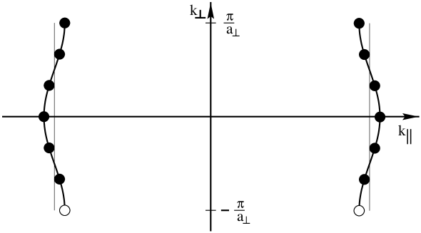
FIG. 1.: Fermi-surface for the model with $N=6$ chains and periodic boundary conditions.

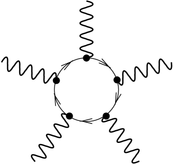
FIG. 2.: Feynman diagram for a closed loop. The solid lines with an arrow represent free Green functions and the wiggled lines represent the auxiliary field $\phi$. The closed loop theorem states that the contributions from all diagrams with more than two auxiliary fields in a closed loop vanish.

REFERENCES

[1] J. Sólyom, Adv. Phys. 28, 201 (1979);
V. J. Emery, in Highly Conducting One-Dimensional Solids, eds
J. T. Devreese, R. P. Evrard and V. E. van Doren, (Plenum, New
York, 1979); F. D. M. Haldane; J. Phys. C 14, 2585 (1981).
[2]
P. A. Lee, T. M. Rice, and R. A. Klemm, Phys. Rev. B 15, 2984 (1977);
X. G. Wen, Phys. Rev. B 42, 6623 (1990);
C. Bourbonnais and L. G. Caron, Int. J. Mod. Phys. B 5, 1033 (1991);
H. J. Schulz, Int. J. Mod. Phys. B 5, 57 (1991);
C. Castellani, C. Di Castro and W. Metzner, Phys. Rev. Lett. 69,
1703 (1992);
F. V. Kusmartsev, A. Luther and A. Nersesyan, JETP Lett. 55, 692 (1992);
A. Nersesyan, A. Luther, and F. V. Kusmartsev, Phys. Lett. A 179, 363
(1993);
M. Fabrizio and A. Parola, Phys. Rev. Lett. 70, 226 (1993); M. Fabrizio, Phys. Rev. B 48, 15838
(1993); A. Finkel’stein and A. I. Larkin, Phys. Rev. B 47, 10461 (1993);
P. Kopietz, V. Meden and K. Schönhammer, Phys. Rev. Lett.
74, 2997 (1995); P. Kopietz, V. Meden and K. Schönhammer,
preprint cond-mat/9701023.
[3] S. Tomonaga, Prog. Theo. Phys. 5, 544
(1950); J. M. Luttinger, J. Math. Phys. 4, 1154 (1963);
D. C. Mattis and E.H. Lieb, J. Math. Phys. 6, 304
(1965).
[4] H. J. Schulz, J. Phys. C 16, 6769 (1983);
K. Penc and J. Sólyom, Phys. Rev. B 47, 6273 (1993).
[5] D. K. K. Lee and Y. Chen, J. Phys. A 21,
4155 (1988).
[6] P. Kopietz, J. Hermisson and K. Schönhammer,
Phys. Rev. B 52, 10877 (1995); P. Kopietz and K. Schönhammer, Z. Phys. B 100, 259 (1996).
[7] I. E. Dzyaloshinskiǐ and A. I. Larkin, Sov. Phys. JETP
38, 202 (1974).
[8] T. Bohr, The Luttinger Model (NORDITA Lecture Notes,
1981),
unpublished.
[9] W. Metzner, C. Castellani, C. Di Castro, to
appear in Adv. Phys. (1997).
[10] Calculations for the model of coupled chains with
finite can be found in L. Bartosch, Diplomarbeit (Göttingen,
Sept. 1996), unpublished.
[11] A. Luther and I. Peschel, Phys. Rev. B
9, 2911 (1974).
[12] N. Shannon, Y. Li, N. d’Ambrumenil, preprint
cond-mat /9611071.
[13]
D. G. Clarke, S. P. Strong, and P. W. Anderson,
Phys. Rev. Lett. 72, 3218 (1994).