Theory for Characterization of Hippocampal Long-Term Potentiation Induced by Time-Structured Stimuli

Abstract

We theoretically investigate long-term potentiation (LTP) in the hippocampus using a simple model of a neuron stimulated by three different time-structured input signals (regular, Markov, and chaotic). The synaptic efficacy change is described taking into account both N-methyl-D-aspartate (NMDA) and non-NMDA receptors. The experimental results are successfully explained by our neuron model, and the remarkable fact that the chaotic stimuli in the nonstationary regime produce the largest LTP is discussed.

1 Introduction

One of the main problems in neuroscience is determining how information is represented in the brain. There have been many experimental and theoretical studies in this direction in the last few years. For example, Aertsen and Gerstein conducted a series of experiments, and proposed the concept of “effective connectivity” [1]. Tsukada et al. showed experimentally that the structure of the inter-spike-interval has a significant effect on the amplitude of long-term potentiation (LTP) in the hippocampus of guinea-pigs, [2] and Fujii et al., based on a large number of experimental data, theoretically proposed the hypothesis of dynamical cell assembly in the central nervous system [3]. However, how information is represented in the brain has not yet been elucidated because the brain is a very complicated and hierarchically organized system. It is necessary to acquire more data about information representation at the neuron level as well as at the network level. It should also be emphasized that determination of how memory information is represented in the brain is essential for understanding of higher brain functions, because all higher brain functions are based on coding of memory information. Furthermore, not only experimental studies but also theoretical studies, involving use of simple biological neuron models or neural networks, are necessary for elucidation of the mechanism of memory information representation and its algorithm.

The purpose of this work was to investigate the effect of the time structure of spike trains on the LTP amplitude in the hippocampus using a simple biological neuron model, and explain the basic synaptic mechanisms underlying memory information representation. For this purpose, we constructed a single neuron model considering both N-methyl-D-aspartate (NMDA) and non-NMDA receptors. Then we applied three different time-structured stimuli (regular, Markov, and chaotic) to our neuron model, and compared the LTP amplitude among the three cases. A striking finding was that the chaotic stimuli in the nonstationary regime produce the largest LTP. This suggests the significance of nonstationary chaotic information representation in memory information processing.

2 Model

Neurons in area CA1 of the hippocampus are typical examples of neurons which exhibit LTP [4, 5]. Since their physiological properties have been extensively studied experimentally, we can construct a single neuron model of this area. Here, we adopt a discrete time model with a continuous membrane potential, a setup, however, which compromises the biological plausibility and the simulation time cost. We take into account the channel properties in the synaptic region.

The basic time evolution of the activity of a single neuron is given by

$$O(t+1)=\left\{\begin{array}[]{ll}1,&\mbox{with prob. $f(V(t))$}\\ 0,&\mbox{with prob. $1-f(V(t))$}\end{array},\right.$$ (1)

where $O(t+1)$ is the output of the neuron at time $t+1$, $V(t)$ is the membrane potential at time $t$, and $f(\cdot)$ is a probability function which describes the relation between the membrane potential and the output. Here, we adopt the following form for $f(\cdot)$:

$$f(V(t))=\frac{1}{1+e^{-(V(t)+|V_{th}|)}},$$ (2)

where $V_{th}$ is the threshold membrane potential ($V_{th}<0$) and $f(V(t))=1/2$ at $V(t)=V_{th}$.

The membrane potential $V(t)$ can be decomposed into three parts, i.e.,

$$V(t)=I(t)+V_{r}+\delta(t),$$ (3)

where $I(t)$ is the post-synaptic potential induced by the input current at time $t$, $V_{r}$ is the constant resting membrane potential, and $\delta(t)$ is a small fluctuation of the membrane potential at time $t$ where the average value of $\delta(t)$ is zero. The synaptic input through non-NMDA receptors $I(t)$ can be represented as follows: $I(t)$ depends on both the synaptic efficacy $E(t)$ and the time course of the input stimulus $\sigma(t)$, which can be written as

$$I(t)=\sum_{n=-\infty}^{t}E(n)\sigma(n)e^{-\alpha(t-n)},$$ (4)

where $E(n)$ is the synaptic efficacy at time $n$, $\sigma(n)$ is the spike train of the input stimuli which represents the existence of the input spike at time $n$ ($\sigma(n)=1$ with input, $\sigma(n)=0$ without input), and $\alpha$ is the decay constant for non-NMDA receptors. The time course of $\sigma(n)$ determines the statistical features of the input signals, such as the average frequency or the average interval of the input stimuli.

Now, let us consider LTP of this model in terms of the change of $E(t)$. Physiologically, both depolarization of the membrane and calcium entry into the post-synaptic neuron are necessary for LTP to occur [4]. Therefore, we introduce the variable $S(t)$, which represents the concentration of calcium ions in the post-synaptic neuron and is expressed as:

$$S(t)=C\sum_{n=-\infty}^{t}\{V(n)+|V_{L}|\}\theta(V(n)+|V_{L}|)e^{-\beta(t-n)},$$ (5)

where $C$ is a constant, $\theta(\cdot)$ is a step function, $V_{L}$ is the membrane potential required for removal of magnesium ions from NMDA receptors ($V_{L}<0$), and $\beta$ is the decay constant for NMDA receptors.

Although it is not well known how the calcium-dependent second messenger system produces LTP, several experimental observations have revealed strong correlation between the LTP amplitude and the frequency of the input stimuli, that is, it is physiologically plausible that (1) regular stimuli at 3 - 10 Hz can induce LTP, [2] but (2) low-frequency stimuli ($\leq$ 1Hz) induce long-term depression (LTD) [6]. We also need to consider that the value of $E(t)$ saturates in the regime of large $S(t)$ and $E(t)$ due to the limited number of neurotransmitters and receptors. Therefore, we propose the following model for the change of the synaptic efficacy $\Delta E(t)$:

$$\Delta E(t) = E(t+1)-E(t)$$

$$= C_{1}(1-e^{-C_{2}(S(t)-C_{3})^{2}})$$

$$\times\left(\frac{1}{1+e^{-C_{4}(-(E(t)-C_{5}))((S(t)-C_{6})-C_{7})}}\right)$$

$$\times\left(\frac{1}{1+e^{-(S(t)-C_{3})}}-C_{8}e^{-C_{9}(S(t)-C_{10})^{2}}\right),$$

where $C_{1},C_{2},C_{3},C_{4},C_{5},C_{6},C_{7},C_{8},C_{9}$, and $C_{10}$ are all parameters. A schematic of $\Delta E(t)$ is given in Fig. 1, where the values of $C_{i}$ are fixed in our simulations.

Figure 1: $\Delta E(t)$ as a function of $E(t)$ and $S(t)$.

For $E(t)\,\,\,\vphantom{(}\lower 4.0pt\hbox{$\stackrel{{\scriptstyle\displaystyle{<}}}{{\sim}}$}\,\,\,20$ and $S(t)\,\,\,\vphantom{(}\lower 4.0pt\hbox{$\stackrel{{\scriptstyle\displaystyle{>}}}{{\sim}}$}\,\,\,10$, $\Delta E(t)$ is positive corresponding to LTP described by the experimental data [2]. For $E(t)\,\,\,\vphantom{(}\lower 4.0pt\hbox{$\stackrel{{\scriptstyle\displaystyle{>}}}{{\sim}}$}\,\,\,20$ and $S(t)\,\,\,\vphantom{(}\lower 4.0pt\hbox{$\stackrel{{\scriptstyle\displaystyle{>}}}{{\sim}}$}\,\,\,10$, $\Delta E(t)$ is zero due to the saturation effect. For $E(t)\,\,\,\vphantom{(}\lower 4.0pt\hbox{$\stackrel{{\scriptstyle\displaystyle{<}}}{{\sim}}$}\,\,\,15$ and $S(t)\,\,\,\vphantom{(}\lower 4.0pt\hbox{$\stackrel{{\scriptstyle\displaystyle{<}}}{{\sim}}$}\,\,\,10$, $\Delta E(t)$ is zero because of less $Ca^{2+}$ entry. For $E(t)\,\,\,\vphantom{(}\lower 4.0pt\hbox{$\stackrel{{\scriptstyle\displaystyle{>}}}{{\sim}}$}\,\,\,15$ and $S(t)\,\,\,\vphantom{(}\lower 4.0pt\hbox{$\stackrel{{\scriptstyle\displaystyle{<}}}{{\sim}}$}\,\,\,10$, $\Delta E(t)$ is negative corresponding to LTD at low frequency [6].

When we consider $N$ neurons which are stimulated independently, the averaged output $<O(t)>$ at time $t$ is defined by

$$<O(t)>=\frac{1}{N}\sum_{i=1}^{N}O_{i}(t),$$ (7)

which can be written as

$$<O(t)>\sim f(V(t))$$ (8)

in a large $N$ limit according to the central limit theorem. Therefore, in this letter we consider $f(V(t))$ to represent the characteristic measure of the LTP amplitude. In Figs. 2 - 4, the amplitude variable of the vertical axis shows $<<f(V(t))>_{t}>_{e}$ for comparison with the physiological data in ref. 2; the notation $<\cdot>_{t}$ represents the time average for a sample process and $<\cdot>_{e}$ represents the ensemble average for a large number of sample processes. In the present letter, the number of ensembles is fixed at $10^{3}$ to $10^{5}$. The values of the parameters used in this letter are chosen to be biologically plausible, i.e., $V_{th}=-55$ mV, $V_{r}=-70$ mV, $\delta(t)$ is generated from the uniform distribution of $-E(0)/100\leq\delta(t)\leq E(0)/100$, $E(0)=15$ mV, $C=0.15$, $V_{L}=-60$ mV, $\alpha=10$ ms, $\beta=200$ ms, $C_{1}=0.00015,C_{2}=0.01,C_{3}=8,C_{4}=0.25,C_{5}=20,C_{6}=4,C_{7}=0.5,C_{8}=0.25,C_{9}=5$, and $C_{10}=1$.

3 Time Structure of the Input Stimuli

To determine the effect of the spike structure on LTP, we consider three different spike stimuli: (i) regular, (ii) Markov, and (iii) chaotic.

For the Markov stimuli, we use the same transition matrix as was used by Tsukada et al. [2] to compare our results with theirs; it is given as

$$P=[P_{ij}]=\left[\begin{array}[]{ccc}SS&SM&SL\\ MS&MM&ML\\ LS&LM&LL\end{array}\right],$$ (9)

where $S$, $M$, and $L$ stand for the Markovian states of the signals with a 100 ms spike interval, 500 ms spike interval, and 900 ms spike interval, respectively. For example, the transition probability $P_{ij}=MS$ indicates that the $S$ (100 ms) interval directly follows the $M$ (500 ms) interval. The transition matrices used in the simulations are given as

$$P_{p}=[P_{ij}]=\left[\begin{array}[]{ccc}0.70&0.20&0.10\\ 0.45&0.10&0.45\\ 0.10&0.20&0.70\end{array}\right]$$ (10)

$$P_{i}=[P_{ij}]=\left[\begin{array}[]{ccc}0.41&0.18&0.41\\ 0.41&0.18&0.41\\ 0.41&0.18&0.41\end{array}\right]$$ (11)

$$\hskip 5.0ptP_{n}=[P_{ij}]=\left[\begin{array}[]{ccc}0.10&0.20&0.70\\ 0.45&0.10&0.45\\ 0.70&0.20&0.10\end{array}\right],$$ (12)

where $P_{p}$, $P_{i}$, and $P_{n}$ correspond to the positive correlation, the independent correlation, and the negative correlation, respectively [2]. The mean frequency of the input stimuli $\sigma(t)$ for all three cases is fixed at 2 Hz.

For the case of chaotic stimuli, we use the modified Bernoulli map $x_{n}\rightarrow x_{n+1}$ (mod.1) to produce the input stimuli $\sigma(t)$,

$$x_{n+1}=\left\{\begin{array}[]{ll}x_{n}+2^{B-1}(1-2\epsilon)x_{n}^{B}+\epsilon,&(0\leq x_{n}\leq 1/2)\\ x_{n}-2^{B-1}(1-2\epsilon)(1-x_{n})^{B}-\epsilon,&(1/2<x_{n}\leq 1),\end{array}\right.$$ (13)

where $1\leq B\leq 3$ and $\epsilon=10^{-13}$ are parameters. Then, in order to fix the mean spike interval at 500 ms (i.e., the mean frequency is 2 Hz), we transform the value of $x_{n}$ to the spike interval $\tau$ of the time course $\sigma(t)$ in the following way:

$$\left\{\begin{array}[]{ccc}0\leq x_{n}<1/9&\rightarrow&\tau=100ms\\ 1/9\leq x_{n}<2/9&\rightarrow&\tau=200ms\\ 2/9\leq x_{n}<3/9&\rightarrow&\tau=300ms\\ 3/9\leq x_{n}<4/9&\rightarrow&\tau=400ms\\ 4/9\leq x_{n}<5/9&\rightarrow&\tau=500ms\\ 5/9\leq x_{n}<6/9&\rightarrow&\tau=600ms\\ 6/9\leq x_{n}<7/9&\rightarrow&\tau=700ms\\ 7/9\leq x_{n}<8/9&\rightarrow&\tau=800ms\\ 8/9\leq x_{n}\leq 1&\rightarrow&\tau=900ms.\end{array}\right.$$ (14)

The properties of this map were thoroughly studied by Aizawa, [7] and it should be noted that the map is stationary chaotic for $B<2$, and nonstationary chaotic for $B\geq 2$. The time course of the input stimuli $\sigma(t)$ generated by eq. (3.6) reveals a typical intermittency for all regimes, and the $1/f$ spectrum is emphasized in the case for $B\geq 2$.

4 Numerical Simulations

Let us now numerically investigate LTP induced by the time-structured stimuli mentioned above. The setup of the numerical LTP experiments is as follows. The unit of the discrete time is taken as 1 ms, and 20 impulses with 0.05 Hz are applied as an initial control stimulus. Then, we ensure that the amplitude $E(t)$ reveals a controlled reference state corresponding to the threshold $V_{th}$. After these preparations, 200 tetanic impulses are applied, and then 20 control impulses with 0.05 Hz intervals (called the latter control) are applied. The LTP amplitude is measured in terms of the average value, $<f(V(t))>_{t}$, where $t$ stands for the duration of the latter control. These procedures for our simulations are the same as in the physiological experiments [2].

The first case is that of the regular periodic stimuli ranging from 10 Hz to 0.5 Hz, and the results are shown in Fig. 2. We use 1,000 different sample processes of stimuli for each frequency, and the ensemble averages of LTP, $<<f(V(t))>_{t}>_{e}$, are shown by the filledcircles and the standard deviations by the errorbars. Figure 2 clearly shows that a higher-frequency stimulus produces a larger LTP than lower-frequency ones, and that no LTP occurs at frequencies of less than 2 Hz. These results are consistent with the results of experiments performed by Tsukada et al. [2]

Figure 2: Amplitude of LTP induced by regular stimuli. One thousand initial conditions are applied to each frequency, and the filledcircles and the errorbars represent the averages and the standard deviations, respectively.

Next, we apply the Markov stimuli produced by the transition matrices in eqs. (3.1), (3.2), and (3.3). For each type of stimulus, we consider 100,000 sample processes, and calculate the average and standard deviation of the LTP amplitude. The results are shown in Fig. 3. It is clear that the positive correlated stimuli produce the largest LTP, the independent ones the next largest ones, and the negative correlated ones the least ones. Comparing Fig. 3 and Fig. 2, we can conclude that the time-structured Markov stimuli with 2 Hz frequency produce a larger LTP than do the regular stimuli with the same frequency. This implies that the time structure of the input signals is important for LTP to occur. Although our result for the independent correlation case does not coincide with the experimental result obtained by Tsukada et al., [2] the positive and the negative cases fit well with their experimental results. Furthermore, our results shown in Figs. 2 and 3 are consistent with the results of previous work performed by Sugiura et al. [8] with a different neuron model.

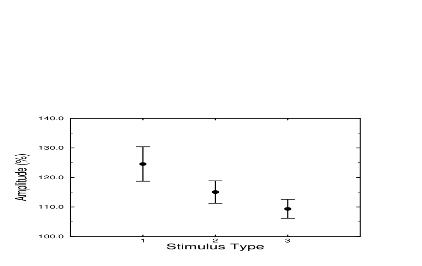
Figure 3: Amplitude of LTP induced by Markov stimuli. The stimulus types 1, 2, and 3 correspond to the positive, the independent, and the negative correlation, respectively. One hundred thousand initial conditions are applied to each type, and the filledcircles and the errorbars represent the averages and the standard deviations, respectively.

Finally, we apply the chaotic intermittent stimuli expressed by eq. (3.6) to our neuron model. For each value of $B$, we produce 10,000 sample processes. The results are shown in Fig. 4. As the value of $B$ increases, the average LTP amplitude increases almost monotonically. Thus we can conclude that on average, the chaotic stimuli in the nonstationary regime produce larger LTP than do the stationary ones. Comparing Fig. 4 with Figs. 2 and 3, we can clearly see that intermittent chaotic stimuli have the strongest LTP effect among all the stimuli, though the fluctuations represented by the standard deviations are also much larger in the nonstationary regime than in the stationary regime.

Figure 4: Amplitude of LTP induced by intermittent chaotic stimuli. Ten thousand initial conditions are applied to each B value, and the filledcircles and the errorbars represent the averages and the standard deviations, respectively.

5 Discussion

In this letter, we proposed a simple neuron model including the effects of NMDA and non-NMDA receptors, and discuss the relation between the time structure of the input stimuli and the amplitude of LTP. It is shown by numerical simulation that the results obtained using our neuron model fit the experimental data reasonably well, and indicate that the chaotic stimuli in the nonstationary regime will produce the largest LTP.

The reason that the time structure of the input stimuli has a significant effect on the amplitude of LTP can be understood by the fact that the calcium concentration through NMDA receptors has a long-lasting memory effect ($\beta=200$ ms), as is shown in eq. (2.5). Thus, if the interval between two spikes is short, the effect of the first spike remains when the second one arrives, resulting in a higher calcium concentration in a post-synaptic neuron. On the other hand, when the interval between the two spikes is long, the effect of the first spike ceases before the second one arrives. Therefore, the inter-spike-interval must be short for LTP to occur in our model. For the Markov stimuli, the positive correlation case has the longest short spike interval, the independent one the next longest, and the negative one the shortest, and this explains the differences in the average LTP amplitude in Fig. 3. In the case for the chaotic stimuli, $x_{n}$ of the modified Bernoulli map tend to localize around $x_{n}\sim 0$ or $x_{n}\sim 1$ in the large $B$ regime, and as the value of $B$ increases, the spikes tend to cluster in a short interval or a long interval for a longer duration. Therefore, if the spikes occur within a short interval for a long duration, they will produce very large LTP. On the other hand, almost no LTP will occur when spikes occur within a long interval for a long duration. This results in the large deviation in the nonstationary regime in Fig. 4. Since the short spike interval becomes longer as the value of $B$ increases, the average LTP amplitude also increases. Moreover, the average LTP amplitude in the nonstationary chaotic regime is the largest among those for all the stimuli, because the short spike interval in the nonstationary chaotic regime is longer than that in any others.

To determine how memory information is represented in the brain, it is necessary to elucidate the relationship between the time structure of the impulse train and its validity as a form of information representation. For this purpose, we obtained the basic data of the LTP formation at the single neuron level. Our results strongly suggest that the time structure of the impulse train is important for memory information representation at the single neuron level. In particular, the result that the nonstationary chaotic spike trains produce the largest LTP implies that the brain may use chaotic intermittency for memory information representation even at the single neuron level. Furthermore, the wide range of the LTP amplitude in the nonstationary regime, which is indicated by the large standard deviation, seems to play a very important role in the selection of the detailed information embedded in the diversity of the time-structured spike trains.

However, in order to acquire the entire pictures of memory information representation and its algorithm in the brain, it is also necessary to determine the relationship between the time structure of the impulse train and its validity as a form of information representation at the network level. Also, in particular, detailed study about the relationship between the time structure of the impulse train and the properties of the network connections, such as symmetric, asymmetric, excitatory, and inhibitory ones, is necessary. To this end, the neuron model proposed in this letter is suitable because it is simple enough for network-level simulation and has biological properties, though some details such as the form of eq. (2.6) can be further simplified. Further research for analysis of the network structure and increasing the level of the sophistication of our neuron model is now in progress.

References

- [1] A. M. H. J. Aertsen and G. L. Gerstein: Neuronal Cooperativity, ed. J. Krüger (Springer-Verlag, Berlin, 1991) p. 52.
- [2] M. Tsukada, T. Aihara, M. Mizuno, H. Kato and K. Ito: Biol. Cybern. 70 (1994) 495.
- [3] H. Fujii, H. Ito, K. Aihara, N. Ichinose and M. Tsukada: Neural Networks 9 (1996) 1303.
- [4] P. S. Churchland and T. J. Sejnowski: The Computational Brain (MIT Press, Cambridge, 1992).
- [5] E. R. Kandel, J. H. Schwartz and T. M. Jessell: Principle of Neuroscience (Appleton & Lange, Norwalk, 1991).
- [6] S. M. Dudek and M. F. Bear: Proc. Natl. Acad. Sci. USA 89 (1992) 4363.
- [7] Y. Aizawa: Prog. Theor. Phys. 99 (1989) 2866.
- [8] Y. Sugiura, T. Aihara and M. Tsukada: Technical Report of IEICE NC93-104 (1994) 181 [in Japanese].