Weakly correlated electrons on a square lattice: a renormalization group theory

Abstract

We study the weakly interacting Hubbard model on the square lattice using a one–loop renormalization group approach. The transition temperature $T_{c}$ between the metallic and (nearly) ordered states is found. In the parquet regime, $(T_{c}\gg|\mu|)$, the dominant correlations at temperatures below $T_{c}$ are antiferromagnetic while in the BCS regime $(T_{c}\ll|\mu|)$ at $T_{c}$ the d-wave singlet pairing susceptibility is most divergent.

A theoretical understanding of systems with two different kinds of coexisting and possibly competing instabilities of density–wave (DW) and superconducting (SC) type remains one of the central problems of the theory of interacting fermions. In particular, the question of a purely electronic mechanism of superconductivity, induced by an incipient instability of the density–wave type, remains difficult if one wants to go beyond the most qualitative level. Typically the existence and strength of the DW correlations and their coupling to superconducting pairing depend strongly on the dimensionality and on the geometry of the Fermi Surface.

Experimentally, superconductivity in the vicinity of an insulating and/or spin density wave state is a well–known property of the phase diagrams for several families of fermion systems: for example, in the quasi–one–dimensional Bechgaard salts,[1] superconductivity (possibly of d–type [2]) replaces an SDW state as one increases pressure, due to two effects: decreasing of the nesting properties of the Fermi surface, and suppression of umklapp scattering between electrons. The phase diagram of the quasi–two–dimensional organic superconductors of the ET family also shows a pressure induced SDW–SC transition [3], but the symmetry of the SC order parameter is not yet clear.[4] In the high–$T_{c}$ superconductors a few percent doping transforms an insulating antiferromagnet into a superconductor[5], probably of the $d_{x^{2}-y^{2}}$ symmetry.[6] In two dimensions the simplest model showing an insulating antiferromagnetic state already at weak coupling is the Hubbard model, often considered as a “minimal model” for high-$T_{c}$ superconductors.[7] Although extensively studied, the question of doping induced superconductivity in the vicinity of the antiferromagnetic state in this model still remains unanswered. In the weak coupling limit the problem of the interdependence of different kinds of instabilities can be treated using renormalization group methods [8, 9], as has been successfully done for the case of quasi–one–dimensional systems[10, 11].

In the present paper we present a one–loop renormalization group analysis of the Hubbard model. Because of its perturbative nature this gives a quantitatively correct phase diagram only for weak coupling and does not allow us to make precise predictions about realistic systems where the coupling is rather strong. However, we are able to describe the physical mechanisms which lead to different instabilities of the model. Provided that there is no transition to a qualitatively different regime for strong repulsion, this should give at least some qualitative insight even outside the strictly perturbative regime, at least for the effective low energy model [8]. Recently we have formulated one–loop renormalization–group equations for the Hubbard model,[9] based on the requirement that the vertex (the effective interaction) must be invariant under changes of the energy cutoff $\Lambda$ about the Fermi surface. This way of renormalization is known as field theory approach.[8] We distinguished two regimes, separated by a crossover energy $T_{co}$ which is a function of the chemical potential $\mu$. In the parquet regime, $\Lambda>T_{co}$, the contributions to the renormalization from the particle-particle and particle-hole loops are both important. In the BCS regime, $\Lambda<T_{co}$, only the particle-particle loop contributes to the flow, while the particle-hole part is negligibly small. In the parquet regime both loops behave like $\log^{2}\Lambda$, while in the BCS regime, the p-p loop crosses over to $\log\Lambda$ and the p-h loop disappears with some positive power of $\Lambda$. For the exactly half–filled case, the parquet equations gave an instability in the antiferromagnetic channel [12]. The same result was found within a simple scaling theory [13] which takes into account only processes between electrons at the van Hove points in the corners of the square Fermi surface. Introducing the chemical potential as a cutoff for the p-h term of the flow equation this theory also gives a transition to d-wave superconductivity.

An important aspect of the renormalization group is that in many cases $\Lambda$ can be interpreted as the temperature to logarithmic precision. This approximation consists in renormalizing the vertex at some temperature $T$ only by virtual processes involving “quantum” electrons, those with energy larger than $T$. Then the vertex depends only on energy variables greater than $T$ and its dependence on energies inside the area $\pm\Lambda$ about the Fermi energy is irrelevant. In that sense the field theoretic approach can give correct thermodynamics only for logarithmic–scale–invariant problems, because in that case the internal fermionic propagators A, A’, B, B’, C, and C’ in fig. 1(a) are all exactly at the energy $\pm\Lambda$ and, consequently, the vertex at the step $\Lambda$ of renormalization contains only contributions from the degrees of freedom outside the ring $\pm\Lambda$. If there is no logarithmic scale invariance, as for the case when $\Lambda>T_{co}\neq 0$, in the field theory approach the lines A,B and C are on the shell, but A’, B’ and C’ can even lie inside the ring $\pm\Lambda$, and $\Lambda$ can thus not be considered as an effective temperature. In order to obtain thermodynamics from the renormalization group we thus have to modify the bookkeeping of mode elimination in a way so that the modes inside the temperature ring $\pm T$ about the Fermi energy never enter the integration. This can be done using the Kadanoff-Wilson mode elimination technique [14] as given by Polchinski’s equations.[15, 16, 17] In the BCS regime, the field theory approach is valid because there only the p-p channel survives and scales just as $\log\Lambda$.

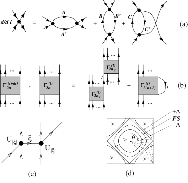
FIG. 1.: (a) The one-loop renormalization of the vertex. (b) The Polchinski equation describes the exact flow of all vertices. The contractions labeled with $l$ are integrated over a phase space shell of energy width $\Lambda d\Lambda$. (c) The 6–leg diagram generated by the first term in Polchinski’s equation. The second term applied to it generates the loops for the renormalization of the 4–leg vertex. (d) The organization of the mode elimination for a non–half–filled case. Dashed lines are the lines of constant “angle” $\theta$.

In this letter we solve Polchinski’s flow equation at the one–loop level, as shown schematically in fig.1. This allows us to find the renormalization of the interaction in the nontrivial case when the proximity of half–filling, via nesting and van Hove singularities, makes both DW and SC tendencies strong and the critical temperature $T_{c}$ can be already in the parquet regime. The renormalization of different correlation functions gives us the phase diagram.

In the Kadanoff–Wilson scheme, the one-loop renormalization flow of the interaction $U(K_{1},K_{2},K_{3},K_{4}(K_{1},K_{2},K_{3}))$ as a function of the three energy-momenta $K_{i}\equiv(\omega_{i},{\bf k}_{i})$ is defined graphically by fig.1(a), where the propagators A, B, and C are on the shell $\pm\Lambda$, but A’, B’, and C’ are constrained to run only over states with $|\xi|\geq\Lambda$. The interactions in the loops are also to be taken at the same cutoff as the propagators A’, B’ and C’ and not at the actual cutoff $\Lambda$. This means that the renormalization of the interaction is nonlocal in $\Lambda$: this is the price we have to pay to get thermodynamics from the renormalization group. For the Hubbard model the initial condition is $U_{\Lambda=\Lambda_{0}}=U$, where $\Lambda_{0}$ is the initial cutoff which we take to be equal to the bandwidth ($=8t$) in order to take degrees of freedom from the whole Brillouin zone into account. It is convenient to introduce the logarithmic scale $l\equiv\ln 8t/\Lambda$.

The fact that $U_{\Lambda}$ is a function of six variables makes the renormalization equations very difficult. Power counting arguments can provide some drastic simplifications, in a way that allows us to eliminate from $U_{\Lambda}$ all irrelevant variables, namely the frequencies $\omega_{i}$ and energy variables $\xi_{\bf k_{i}}$ of the interacting particles. A problem with scaling in the parquet regime with $\mu\neq 0$ is that if one chooses processes exactly at the Fermi surface as marginally relevant, the nesting and umklapp scattering processes appear formally as irrelevant, whereas this irrelevancy only really occurs when $\Lambda\ll|\mu|$, i.e. in the BCS regime. On the other hand, the irrelevance of the energy variables allows us to choose as marginally relevant a set of processes between electrons at any distance from the Fermi surface in the ring $\pm\Lambda$, not necessarily at the Fermi surface. Thus, in the parquet regime we keep nesting and umklapp processes even for $\mu\neq 0$ by considering processes between electrons exactly at the square Fermi surface of the half–filled case. Up to irrelevant corrections $U$ then depends only on projections of the momenta on this square, as shown in Fig. 1(d), i.e. $U_{\Lambda}=U_{\Lambda}(\theta_{1},\theta_{2},\theta_{3})$. On the other side of the crossover, in the BCS regime there remains only the BCS amplitude $V_{\Lambda}(\theta_{1},\theta_{3})=U_{\Lambda}(\theta_{1}=\theta_{2}+\pi,\theta_{3}=\theta_{4}+\pi)$, but now the particles are at the Fermi surface, and not on the square, since the square is outside the ring $\pm\Lambda$.

The renormalization equation for the interaction as function of $\theta_{i}$ only is of the same form as in ref.[9], but now with

$$\beta_{ee}\{U,U\}(\theta_{1},\theta_{2},\theta_{3})=\Xi\{U,U\}(\theta_{1},\theta_{2},\theta_{3})+\Xi\{XU,XU\}(\theta_{1},\theta_{2},\theta_{3})$$ (1)

and

$$\beta_{eh}\{U_{1},U_{2}\}(\theta_{1},\theta_{2},\theta_{3})=\Pi\{U_{1},U_{2}\}(\theta_{1},\theta_{2},\theta_{3})+\Pi\{U_{1},U_{2}\}(\theta_{3},\theta_{4},\theta_{1}),$$ (2)

where

$$\Xi\{U,U\}(\theta_{1},\theta_{2},\theta_{3})=\frac{-2}{(2\pi)^{2}}\sum_{\nu=+,-}\int d\theta{\cal J}(\nu\Lambda,\theta)$$

$$\frac{\Theta\left(\nu\xi_{{\bf k}_{\nu}-{\bf q}_{ee}}\right)\Theta\left(|\xi_{{\bf k}_{\nu}-{\bf q}_{ee}}|-\Lambda\right)}{1+\frac{\nu}{\Lambda}\xi_{{\bf k}_{\nu}-{\bf q}_{ee}}}\times$$

$$\times U_{|\xi_{{\bf k}_{\nu}-{\bf q}_{ee}}|}(\theta_{1},\theta_{2},\theta)U_{|\xi_{{\bf k}_{\nu}-{\bf q}_{ee}}|}(\theta_{3},\theta_{4},\theta)\;,$$ (3)

$$\Pi\{U_{1},U_{2}\}(\theta_{1},\theta_{2},\theta_{3})=\frac{2}{(2\pi)^{2}}\sum_{\nu=+,-}\int d\theta{\cal J}({\nu}\Lambda,\theta)$$

$$\frac{\Theta\left(-\nu\xi_{{\bf k}_{\nu}+{\bf q}_{eh}}\right)\Theta\left(|\xi_{{\bf k}_{\nu}+{\bf q}_{eh}}|-\Lambda\right)}{1-\frac{\nu}{\Lambda}\xi_{{\bf k}_{\nu}+{\bf q}_{eh}}}\times$$

$$\times U_{1,|\xi_{{\bf k}_{\nu}+{\bf q}_{eh}}|}(\theta_{1},\theta,\theta_{3})U_{2,|\xi_{{\bf k}_{\nu}+{\bf q}_{eh}}|}(\theta_{4},\theta,\theta_{2})\;.$$ (4)

${\bf k}_{\nu}$ is the momentum of a particle at angle $\theta$ with energy $\xi=\nu\Lambda$. ${\cal J}(\epsilon,\theta)\equiv J[(x,y)/(\epsilon,\theta)]$ is the Jacobian of the transformation from rectangular coordinates in momentum space to the polar ones. $X$ is the exchange operator defined as $XU(\theta_{1},\theta_{2},\theta_{3})=U(\theta_{2},\theta_{1},\theta_{3})$. $U_{1}$ and $U_{2}$ in the expression (4) symbolize $U$ or $XU$ as given in ref. [9]. Note that the interactions $U$, $U_{1}$, and $U_{2}$ in the expressions (3) and (4) are not at the actual cutoff $\Lambda$, but at a cutoff given by the configuration of external legs and the integration momentum ${\bf k}_{\nu}$ (entering via total momentum ${\bf q}_{ee}={\bf k}_{1}+{\bf k}_{2}$ and momentum transfer ${\bf q}_{eh}={\bf k}_{1}-{\bf k}_{3}$). To solve the renormalization equations we have discretized the $\theta$–dependence of the interaction, approximating in that way the function $U_{\Lambda}(\theta_{1},\theta_{2},\theta_{3})$ by a set of coupling constants $U_{\Lambda}(i_{1},i_{2},i_{3})$. Fig.2 shows the flow of some of the 93 coupling constants for the case of a discretization in 16 patches. There is one pole at $l_{c}=\ln(8t/\Lambda_{c})$, determined by the initial interaction and the chemical potential, and in this case it is in the parquet regime. All coupling constants which have logarithmic corrections diverge for $l=l_{c}$. We identify this point as the critical temperature $T_{c}=8t\exp(-l_{c})$ in a mean field sense. The critical temperature at half–filling, $T_{c}^{0}$ is slightly inferior to the mean-field one, but the ratio $l_{c}^{MF}/l_{c}=0.985$ does not depend on the strength of the interaction. As one sees in fig.3, $T_{c}$ is finite for any filling, in contrast to mean–field calculations where $T_{c}$ falls to zero at a threshold doping given approximately by $|\mu|=T_{c}^{0}$.

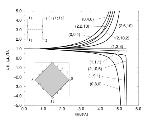
FIG. 2.: The flow of a few typical (among 93) scattering amplitudes for a Fermi surface covered by 16 patches, for chemical potential $\mu=8t\exp(-7.8)$ and initial interaction $U=4t/3$.

To determine the dominant fluctuations at $T=T_{c}$, we calculate the correlation matrices for antiferromagnetism $\chi^{SDW}(\theta_{1},\theta_{2})$ and for superconductivity $\chi^{SC}(\theta_{1},\theta_{2})$, defined as

$$\chi_{\bf q}^{\delta}(\theta_{1},\theta_{2};|\tau_{1}-\tau_{2}|)=\int_{>}d\epsilon_{1}\int_{>}d\epsilon_{2}\;{\cal J}(\epsilon_{1},\theta_{1}){\cal J}(\epsilon_{2},\theta_{2})$$

$$\langle\hat{\Delta}_{\bf q}^{\delta}(\epsilon_{1},\theta_{1};\tau_{1})\bar{\hat{\Delta}}_{\bf q}^{\delta}(\epsilon_{2},\theta_{2};\tau_{2})\rangle,$$ (5)

with $\delta=SC,SDW$. The symbols “$>$” mean that the energy integrals are over energies outside of the shell $\pm\Lambda$. Consequently, $\chi^{SC}$ and $\chi^{SDW}$ have the interpretation of the susceptibilities at the temperature $T=\Lambda$. At the beginning of the renormalization when $\Lambda=\Lambda_{0}=8t$ both susceptibilities are zero.

The order parameter variables are

$$\hat{\Delta}_{\bf q}^{SC}(\epsilon,\theta;\tau)\equiv\sum_{\sigma}\sigma\Psi_{\sigma,{\bf k}}(\tau)\Psi_{-\sigma,-{\bf k}+{\bf q}}(\tau),$$ (6)

$$\hat{\Delta}_{\bf q}^{SDW}(\epsilon,\theta;\tau)\equiv\sum_{\sigma}\bar{\Psi}_{\sigma,{\bf k}}(\tau)\Psi_{-\sigma,{\bf k}+(\pi,\pi)+{\bf q}}(\tau),$$ (7)

where k is given by the angle $\theta$ and the energy $\epsilon$. We consider only the static and long–wavelength limit and follow the renormalization of the maximal eigenvalues of both correlation matrices; in the SDW channel the corresponding eigenvector belongs to the $A_{1}$ representation ($s$–wave), while superconductivity has $B_{1}$ symmetry ($d_{x^{2}-y^{2}}$–wave). For low doping (small $\mu$) the divergence at $\Lambda=T_{c}$ occurs in the magnetic channel (the “SDW” region in fig. 3).

FIG. 3.: The phase diagram.

For higher doping, the pairing susceptibility diverges first, i.e. the “d–wave” region is a $d_{x^{2}-y^{2}}$ superconductor. The triple point metal–SDW–superconductor is at the crossover line $T\approx|\mu|$. As we are considering a two–dimensional system here one should be careful about the interpretation of $T_{c}$: in the case of magnetism, this indicates the onset of well–defined finite–range correlations. For weak interactions, this is typically a very well–defined crossover.[18] In the case of pairing $T_{c}$ can be identified with the onset of quasi–long–range order.

In our calculations we have neglected self-energy corrections which are in Polchinski’s formalism given by Hartree–Fock like terms with renormalized $\omega$ and q dependent vertices. The broadening and redistribution of the spectral weight of the quasiparticles is then determined by the dynamics of the vertex, which is irrelevant in lowest order by power counting and is therefore neglected. One should however notice that at the two–loop order self–energy effects do become important, as known from the one–dimensional case.[10] In that sense, our $T_{c}$ should be understood as a temperature where the effects of interaction start to change strongly not only the two–particles correlations, but the single particle properties as well.

Using the above results and arguments, a more detailed description of the phase diagram, fig.3, can be given: the transition between Fermi liquid and the magnetic phase occurs in the parquet regime. Here the precursor effects, divergence of the commensurate SDW correlation function and relevance of umklapp processes, suggest that $T_{c}$ is the temperature of a metal-insulator transition occurring together or very close to a magnetic instability. For a more specific description of this phase one should include self–energy terms. In the pairing phase (d–wave in fig.3) one expects a spin-gap, due to the formation of d–wave singlets, as one sees from the renormalization the pairing correlations. The maximum pairing temperature is about $T_{c}^{0}/4$, in fact quite close to conserving approximation calculations [19] and to the experimental value of about 1/6 in lanthanum high–$T_{c}$ compounds.[5] The $d_{x^{2}-y^{2}}$ symmetry of the pairing is also in agreement with the majority of experiments in cuprates. [6]

From large N arguments[8, 9] we know that the self–energy corrections will disappear as $T_{c}/t$ if $T_{c}$ is deeply in the BCS regime. Consequently, far from half filling[9], $T_{c}$ is a very good approximation for a superconducting transition, stabilized already by an infinitesimal inter–plane hopping. Finally, mean-field arguments[17] suggest that one expects an incommensurate SDW only in the BCS regime, where perfect nesting is impossible. However, the precision of our calculation (we cut the Brillouin zone into up to 24 $\theta$-patches) is not sufficient to check whether a magnetic correlation function diverges at $T_{c}$ at some incommensurate wave vector.

In conclusion, we have investigated the two–dimensional Hubbard model using a perturbative renormalization group approach. This allows us to treat instabilities in the particle–particle and particle–hole channels on an equal footing and in particular to address the important question of superconductivity induced by spin fluctuations. In the vicinity of half–filling we do indeed find a sizeable superconducting transition temperature, about one fourth of the typical magnetic energy scale. The pairing is of the $d_{x^{2}-y^{2}}$ type.

- [1] D. Jérome and H. J. Schulz, Adv. Phys., 31, 299 (1982); D. Jérome, in “Organic Conductors”, ed. J. P. Farges (Marcel Dekker, New York, 1994), p. 405.
- [2] M. Takigawa, H. Yasuoka and G. Saito, J. Phys. Soc. Jpn. 56, 873 (1987).
- [3] J. E. Schirber et al., Phys. Rev. B 44, 4666 (1991); H. Mayaffre et al., Europhys. Lett. 28, 205 (1994); K. Miyagawa et al., Phys. Rev. Lett. 75, 1174 (1995).
- [4] D. R. Harshman et al., Phys. Rev. Lett. 64, 1293 (1990); J. P. Le et al., Phys. Rev. Lett. 68, 1923 (1992); H. Mayaffre et al., Phys. Rev. Lett. 75, 4122 (1995).
- [5] “Physical Properties of High temperature Superconductors”, vol. 1–5, ed. by D. M. Ginsberg (World Scientific, Singapore); “High Temperature Superconductivity: The Los Alamos Symposium 1989”, ed. by K. S. Bedell et al. (Addison Wesley, redwood City, 1990).
- [6] D. A. Wollman et al., Phys. Rev. Lett. 74, 797 (1995); J. R. Kirtley et al., Nature (London) 373, 225 (1995); Z.-X. Shen et al., Science 267, 343 (1995); R. C. Dynes, Solid State Commun., 92, 53 (1994); W. N. Hardy et al., Phys. Rev. Lett. 70, 3999 (1993); J. A. Martindale et al., Phys. Rev. B47, 9155 (1993); D. J. Scalapino, Phys. Rep. 250, 329 (1995).
- [7] P. W. Anderson, Science 235, 1196 (1987).
- [8] R. Shankar, Rev. Mod. Phys. 66, 129 (1994).
- [9] D. Zanchi and H. J. Schulz, Phys. Rev. B 54, 9509 (1996).
- [10] V. J. Emery, in “Highly Conducting One–Dimensional Solids”, eds. J. T. Devreese, R. P. Evrard and V. E. Van Doren (Plenum, New York 1979), p. 247; J. Sólyom, Adv. Phys. 28, 201 (1979).
- [11] C. Bourbonnais and L. G. Caron, Int. J. Mod. Phys. 5, 1033 (1991).
- [12] I. E. Dzyaloshinskii, Sov. Phys. JETP 66, 848 (1987); I. E. Dzyaloshinskii and V. M. Yakovenko, Sov. Phys. JETP 67, 844 (1988).
- [13] H. J. Schulz, Europhys. Lett. 4, 609 (1987).
- [14] S. K. Ma, Modern Theory of Critical Phenomena, Benjamin (1976).
- [15] J. Polchinski, Nucl. Phys. B231, 269 (1984).
- [16] T. R. Morris, Int. J. Mod. Phys. A9, 2411 (1994).
- [17] D. Zanchi, Ph.D. thesis, Université Paris-Sud (1996) (unpublished).
- [18] H. J. Schulz, Phys. Rev. B 39, 2940 (1989).
- [19] N. E. Bickers, D. J. Scalapino, and S. R. White, Phys. Rev. Lett. 62, 961 (1989).