Transfer-Matrix Study of Hard-Core Singularity
for Hard-Square Lattice Gas

Abstract

A singularity on the negative fugacity axis of the hard-square lattice gas is investigated in terms of numerical diagonalization of transfer matrices. The location of the singular point $z_{\rm c}^{-}$ and the critical exponent $\nu$ are accurately determined by the phenomenological renormalization technique as $-0.11933888188(1)$ and $0.416667(1)$, respectively. It is also found that the central charge $c$ and the dominant scaling dimension $x_{\sigma}$ are $-4.399996(8)$ and $-0.3999996(7)$, respectively. These results strongly support that this singularity belongs to the same universality class as the Yang-Lee edge singularity ($c=-\frac{22}{5}$, $x_{\sigma}=-\frac{2}{5}$ and $\nu=\frac{5}{12}$).

1 Introduction

For systems of hard particles, the radius of convergence of the fugacity series expansion is known to be generally determined by a non-physical singularity on the negative real fugacity $z$ axis [1, 2, 3, 4]. Here, let us consider the hard-square lattice gas (hard squares), which is one of the simplest models describing the fluid-solid transition in two dimensions. This model exhibits a second-order transition at

$$z_{\rm c}^{+}=3.796255174(3)$$ (1)

from the disordered phase to the $\sqrt{2}\times\sqrt{2}$ phase [5] (uncertainty in the last decimal digits is given by the figure in parentheses). It is also precisely confirmed that the transition belongs to the same universality class as the Ising ferromagnet [6].

On the other hand, the alternating behavior in the sign of the coefficients in the fugacity series of the reduced pressure [7]:

$$P = z-\frac{5}{2}z^{2}+\frac{31}{3}z^{3}-\frac{209}{4}z^{4}+\frac{1476}{5}z^{5}-\frac{10739}{6}z^{6}$$

$$\ \mbox{}+\frac{79780}{7}z^{7}-\frac{601905}{8}z^{8}+\frac{4595485}{9}z^{9}-\cdots$$

manifests that a dominant singularity exists on the negative fugacity axis. By series analysis [8], the location of the singularity is estimated as

$$z_{\rm c}^{-}=-0.1193388809(10).$$ (3)

Note that the absolute magnitude of $z_{\rm c}^{-}$ is about 30 times smaller than that of $z_{\rm c}^{+}$. This fact makes it quite difficult to derive precise information around the physical critical point $z_{\rm c}^{+}$ from the fugacity series [2]. Similar situations are commonly observed in other hard-core systems.

This non-physical singularity is referred to as the hard-core singularity or the repulsive-core singularity. At this point thermodynamic quantities are known to exhibit interesting non-trivial behavior. For example, the reduced pressure or equivalently the reduced free-energy density behaves as

$$-P(z)=f(z)\sim(z-z_{\rm c}^{-})^{\phi}$$ (4)

for $z\rightarrow z_{\rm c}^{-}+$. The singularity is characterized by the exponent $\phi$. For the hard-square lattice gas $\phi$ is found to be about $0.83337$ by series analysis [8].

In 1984, Poland [9] investigated the fugacity series for a variety of hard-core lattice gases and hard-core gases in continuous space in two, three and higher dimensions, and proposed that the exponent $\phi$ is universal, that is, it depends only on the dimensionality of space. Another study on further models by Baram and Luban [10] also supports this conjecture.

In addition, Lai and Fisher [11] pointed out that the hard-core singularity can be identified with the Yang-Lee edge singularity [12, 13, 14, 15, 16, 17] (the exponent $\phi$ of the hard-core singularity relates to Fisher’s exponent $\sigma$ of the Yang-Lee edge singularity by $\phi=\sigma+1$). It means, if it is true, that the singular point $z=z_{\rm c}^{-}$ can be regarded as a conventional critical point; the correlation length diverges and consequently ordinary finite-size scaling analysis does work.

As far as we know, all the studies with respect to the hard-core singularity are done by means of series analysis up to the present time (except for the analytic solution for hard hexagons [10, 18] and the trivial cases in dimensions less than two). In this paper, we investigate this singularity of the hard-square lattice gas by another approach — numerical diagonalization of transfer matrices and phenomenological renormalization analysis.

The transfer-matrix method is one of the most powerful numerical methods in investigating statistical mechanical models in low dimensions [19]. It has some advantages such as the absence of statistical errors and critical slowing down, which are observed in Monte Carlo simulations. Moreover, in two dimensions, the conformal invariance associated with a critical system yields a great deal of interesting consequences [20, 21, 22]. Especially, useful asymptotically exact relations between universal quantities, such as the critical exponent, and eigenvalues of the transfer matrix are given. This enables us to perform precise analysis about the criticality even in the non-unitary case with a negative central charge, such as the present hard-core singularity, as shown later.

The organization of the present paper is as follows: In §2 we describe the transfer-matrix method and give the explicit notation of the transfer matrix for the hard-square lattice gas. In §3 the critical point of the hard-core singularity and some universal quantities are investigated by means of the phenomenological renormalization technique. In addition, in §4 we consider the critical eigenvalue spectrum of the transfer matrix precisely, which relates to the operator content of the corresponding conformal theory. We give a summary and some discussion in the final section.

2 Transfer Matrix for Hard-Square Lattice Gas

The partition function of the hard-square lattice gas is defined as follows:

$$Z=\sum_{\{s_{i}\}}z^{\sum_{i}s_{i}}\prod_{\langle i,j\rangle}(1-s_{i}s_{j}),$$ (5)

where $s_{i}$ is a one-bit binary number, which describes whether the $i$th site on the square lattice is occupied ($s_{i}=1$) or vacant ($s_{i}=0$). The product in eq. (5) runs over all nearest-neighbor pairs of the lattice sites. The size of hard squares is so that any two of them can not occupy on nearest-neighbor positions simultaneously.

The partition function of the system of $L\times M$ sites with periodic boundary conditions can be expressed in terms of the transfer matrix [19]:

$$Z_{LM}={\rm Tr}\ (T_{L})^{M}.$$ (6)

The transfer matrix $T_{L}$ is square and of order $2^{L}$. Note there remains some options in choosing the transfer direction and dividing the total Hamiltonian into a sum of slice Hamiltonians [19]. In this paper, we consider the following two types of transfer matrices, which have distinct transfer directions with each other.

2.1 Row-to-row transfer matrix

The first one is the row-to-row transfer matrix. The transfer direction is chosen to be parallel to a set of lattice edges (Fig. 1 (a)). The $(\tau|\sigma)$ element is explicitly written as

$$T_{{\rm r},L}(\tau|\sigma)=z^{\sum_{i=1}^{L}s_{i}}\prod_{i=1}^{L}(1-s_{i}s_{i+1})(1-s_{i}t_{i})(1-t_{i}t_{i+1}),$$ (7)

where $\sigma=(s_{1},s_{2},\cdots,s_{L})$ and $\tau=(t_{1},t_{2},\cdots,t_{L})$ respectively denote one of $2^{L}$ configurations on the two neighboring unit slices respectively ($s_{i}$, $t_{i}=1$ or 0). Periodic boundary conditions along the unit slices (the vertical direction in Fig. 1 (a)) are applied ($s_{i+L}=s_{i}$ and $t_{i+L}=t_{i}$).

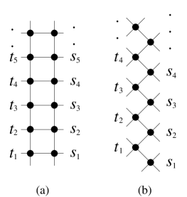
Figure 1: Two neighboring unit slices of the row-to-row (a) and the diagonal-to-diagonal (b) transfer matrices. The transfer direction is chosen in the horizontal direction (right to left) in both cases. In the vertical direction, periodic boundary conditions are applied.

It should be noticed that quite a number of matrix elements should vanish owing to the presence of the hard-core interaction. Especially, the number of rows or columns containing at least one non-zero element is only $\left(\frac{1}{2}(1+\sqrt{5})\right)^{L}=(1.61803\cdots)^{L}$ for $L\gg 1$. This is much smaller than $2^{L}$. One can construct an algorithm for multiplication of the matrix to a trial vector almost in this highly restricted space as shown by Todo and Suzuki [6]. Thus, dominant eigenvalues of the transfer matrix can be calculated effectively up to the system width $L=28$, which is quite larger than that achieved by the standard sparse-matrix factorization [5, 23].

2.2 Diagonal-to-diagonal transfer matrix

We also consider the diagonal-to-diagonal transfer matrix. In this case, the transfer direction is rotated by the amount of $\frac{\pi}{4}$ to a set of lattice edges (Fig. 1 (b)). Periodic boundary conditions are also applied in the orthogonal direction. Matrix elements are written as follows:

$$T_{{\rm d},L}(\tau|\sigma)=z^{\sum_{i=1}^{L}s_{i}}\prod_{i=1}^{L}(1-s_{i}t_{i})(1-s_{i+1}t_{i}),$$ (8)

In this case, any two particles on the sites in a unit slice do not interact with each other. Consequently, all the rows or columns of the matrix $T_{{\rm d},L}$ contains at least one none-zero element. By using the standard sparse-matrix factorization technique [5, 23], numerical matrix multiplication to a vector can be carried out up to $L=20$.

2.3 Eigenvalues, free-energy density and correlation length

In the $M\rightarrow\infty$ limit, the reduced free-energy density $f_{L}$ is given in terms of the largest eigenvalue $\lambda_{1}$ of the transfer matrix as

$$f_{L} = \lim_{M\rightarrow\infty}\left(-\frac{1}{LM}\log Z_{LM}\right)$$ (9)

$$= -\frac{1}{L}\log\lambda_{1}.$$

The inverse correlation length in the transfer direction, which is also referred to as the gap, is calculated as

$$\xi_{L}^{-1}=g_{L}=\log\left|\frac{\lambda_{1}}{\lambda_{2}}\right|,$$ (10)

where $\lambda_{2}$ is the second largest eigenvalue in absolute magnitude.

It should be noted that for $z<0$ a number of matrix elements in eqs. (7) and (8) become negative. Consequently, there is no guarantee that the largest eigenvalue is unique. In general, it may appear as a member of degenerating eigenvalues or one of a complex-conjugate pair. It is in a sharp contrast to the case for $z>0$, where the largest eigenvalue is always real and non-degenerate as a consequence of the Perron-Frobenius theorem [24].

However, in the present case, one can easily show that there exists a certain fugacity region ($z_{L}^{\times}<z<0$), where the largest eigenvalue is actually real and non-degenerate, as the following:

First of all, note that all the elements of $T_{{\rm r},L}$ and $T_{{\rm d},L}$ are real. Then, it is apparent coefficients of their characteristic polynomials are all real. This means that imaginary eigenvalues should appear as complex-conjugate pairs, if they exist. On the other hand, it can be easily seen that at $z=0$ the largest eigenvalue is unity and all the other eigenvalues are zero. Consequently, the largest eigenvalues is real and non-degenerate at least between the $z=0$ and the point $z=z_{L}^{\times}$, where the largest and the second-largest eigenvalues first cross with each other [25]. For $z<z_{L}^{\times}$, they form a complex-conjugate pair. In the following, we work only in the region $z_{L}^{\times}<z<0$.

Table 1: Critical point $z_{L}^{*}$, exponent $\nu_{L}$, scaled gap $Lg_{L}(z)/2\pi$ at $z_{L}^{*}$ and central charge $c_{L}$ for the row-to-row transfer matrix. Their extrapolated values to $L\rightarrow\infty$ are also listed in the bottom row.

$L$	$z^{*}_{L}$	$\nu_{L}$	$Lg_{L}/2\pi$	$c_{L}$
2	-0.11569699529389	0.421849529	0.4814837782	0.417414138
3	-0.11856124181461	0.416582977	0.4394700591	0.438343788
4	-0.11908596327934	0.415750210	0.4233109453	0.430386102
5	-0.11923864086390	0.415659639	0.4150498994	0.421997003
6	-0.11929304185438	0.415705242	0.4104150242	0.416258939
7	-0.11931538407218	0.415775276	0.4076315079	0.412555119
8	-0.11932569455336	0.415846360	0.4058502112	0.410099405
9	-0.11933093621984	0.415912883	0.4046435075	0.408387975
10	-0.11933381954516	0.415973444	0.4037860694	0.407135062
11	-0.11933550958958	0.416027918	0.4031528434	0.406179637
12	-0.11933655239965	0.416076654	0.4026705275	0.405427508
13	-0.11933722350045	0.416120179	0.4022938659	0.404820630
14	-0.11933767079976	0.416159066	0.4019936087	0.404321316
15	-0.11933797791846	0.416193868	0.4017501012	0.403903960
16	-0.11933819423819	0.416225088	0.4015496991	0.403550501
17	-0.11933835002255	0.416253176	0.4013826680	0.403247800
18	-0.11933846442079	0.416278521	0.4012418994	0.402986066
19	-0.11933854989180	0.416301464	0.4011220978	0.402757844
20	-0.11933861474296	0.416322296	0.4010192489	0.402557360
21	-0.11933866463558	0.416341268	0.4009302622	0.402380074
22	-0.11933870350381	0.416358598	0.4008527257	0.402222367
23	-0.11933873413008	0.416374471	0.4007847341	0.402081322
24	-0.11933875851387	0.416389050	0.4007247649	0.401954561
25	-0.11933877811309	0.416402474	0.4006715898	0.401840128
26	-0.11933879400494	0.416414865	0.4006242084	0.401736403
27	-0.11933880699512	0.416426329	0.4005817991	0.401642027
$\infty$	-0.11933888189(2)	0.416668(2)	0.3999996(7)	0.400000(2)

Table 2: Critical point $z_{L}^{*}$, exponent $\nu_{L}$, scaled gap $Lg_{L}(z)/2\pi$ at $z_{L}^{*}$ and central charge $c_{L}$ for the diagonal-to-diagonal transfer matrix. Their extrapolated values to $L\rightarrow\infty$ are also listed in the bottom row.

$L$	$z^{*}_{L}$	$\nu_{L}$	$Lg_{L}/2\pi$	$c_{L}$
2	-0.11876248705617	0.447460528	0.4308877716	0.320446273
3	-0.11923273442241	0.431550594	0.4126164837	0.355461268
4	-0.11930719600997	0.425758018	0.4068301638	0.370796613
5	-0.11932661625882	0.422898114	0.4042554292	0.379106387
6	-0.11933327955420	0.421248828	0.4028891193	0.384181172
7	-0.11933601031532	0.420200952	0.4020795070	0.387534567
8	-0.11933727916302	0.419489095	0.4015617111	0.389879246
9	-0.11933792672807	0.418981068	0.4012113921	0.391590106
10	-0.11933828221945	0.418604487	0.4009639003	0.392880960
11	-0.11933848910493	0.418316797	0.4007829378	0.393881552
12	-0.11933861540512	0.418091545	0.4006468626	0.394674591
13	-0.11933869564988	0.417911541	0.4005421319	0.395314964
14	-0.11933874838811	0.417765191	0.4004599259	0.395840334
15	-0.11933878407038	0.417644431	0.4003943056	0.396277293
16	-0.11933880882938	0.417543502	0.4003411561	0.396645072
17	-0.11933882639297	0.417458199	0.4002975557	0.396957882
18	-0.11933883909801	0.417385385	0.4002613844	0.397226416
19	-0.11933884844969	0.417322683	0.4002310753	0.397458855
$\infty$	-0.11933888188(1)	0.416667(1)	0.3999994(9)	0.399999(1)

3 Phenomenological Renormalization

The largest and the second-largest eigenvalues of the transfer matrix are calculated by the power method [26] up to $L=28$ and $L=20$ for the row-to-row and diagonal-to-diagonal transfer matrices, respectively. In the present case, other improved variations of the power method such as the conjugate-gradient method or the Lanczós method [27] are found to be less numerically stable. In the computation, we use quadratic-precision real numbers instead of double-precision numbers, so that finite-size quantities ($z_{L}^{*}$ in eq. (11), etc.) can be obtained with the uncertainty of $10^{-20}$ or less. As seen below, finite-size data exhibit quite rapid convergence to the thermodynamic limit. Then, the quite high accuracy for them is required to make meaningful extrapolations.

The critical point is estimated by solving the phenomenological renormalization equations:

$$Lg_{L}(z^{*}_{L})=L^{\prime}g_{L^{\prime}}(z^{*}_{L})$$ (11)

for two successive system sizes $L$ and $L^{\prime}=L+1$. As shown in Table I and II, there is no alternating behavior in finite-size corrections with respect to the parity of $L$. It is in contrast with the case for the physical critical point at $z=z_{\rm c}^{+}$, where the systems with even and odd width have different finite-size corrections with each other, reflecting the anti-ferromagnetic-like $\sqrt{2}\times\sqrt{2}$ ordering in the ordered phase [6]. Then, iterated fits [5] of 3rd order yields

$$z_{\rm c}^{-}=-0.11933888189(2)\\$$ (12)

for the row-to-row transfer matrix and

$$z_{\rm c}^{-}=-0.11933888188(1)\\$$ (13)

for the diagonal-to-diagonal one. They agree excellently with each other. They are also consistent with eq. (3), but much accurate by about two orders of magnitude.

The exponent $\nu$ can be found from derivatives of the gap:

$$1/\nu_{L}=\frac{\log\left(\left.\frac{dg_{L^{\prime}}}{dz}\right/\frac{dg_{L}}{dz}\right)}{\log(L^{\prime}/L)}+1$$ (14)

at $z=z_{L}^{*}$. The results are also listed in Table I and II. They are extrapolated to the thermodynamic limit by iterated fits as

$$\nu=0.416668(2)$$ (15)

and

$$\nu=0.416667(1)$$ (16)

in the row-to-row and diagonal-to-diagonal cases, respectively. These results indicate $\nu=\frac{5}{12}$, which is expected to be exact for the Yang-Lee edge singularity in two dimensions [16].

At the critical point, the scaled gap $Lg_{L}(z)$ in eq. (11) is believed to be universal [28, 29], that is,

$$Lg_{L}(z_{\rm c}^{-})=2\pi x_{\sigma}$$ (17)

for $L\rightarrow\infty$, where $x_{\sigma}$ would be the scaling dimension of the dominant scaling operator and relate to the exponent of the correlation function $\eta$ by $\eta=2x_{\sigma}$. It is also expected that the coefficient of the leading finite-size correction to the critical free-energy density becomes universal [30, 31]:

$$f_{L}(z_{\rm c}^{-})=f_{0}-\frac{\pi c}{6L^{2}}+\cdots,$$ (18)

where $f_{0}$ is the critical free-energy density of the bulk, and $c$ is the central charge of the Virasoro algebra, which characterize the critical theory of the model [20].

In practice, finite-size estimates for $x_{\sigma}$ and $c$ are calculated by

$$x_{\sigma,L}=\frac{1}{2\pi}Lg_{L}(z_{L}^{*})$$ (19)

and

$$c_{L}=\frac{6}{\pi}\frac{L^{2}L^{{}^{\prime}2}}{(L^{{}^{\prime}2}-L^{2})}\{f_{L^{\prime}}(z_{L}^{*})-f_{L}(z_{L}^{*})\},$$ (20)

respectively. As seen in Table 1 and 2, both of $x_{\sigma,L}$ and $c_{L}$ tend to rapidly converge to the same value $\frac{2}{5}$ for $L\rightarrow\infty$. The best estimates are

$$c=0.399999(1)$$ (21)

and

$$x_{\sigma}=0.3999996(7),$$ (22)

respectively. Following these results, one may conclude that the singularity at $z=z_{\rm c}^{-}$ would be described by a conformal field theory with $c=\frac{2}{5}$ and $x_{\sigma}=\frac{2}{5}$. However, this theory does not appear in the classification of the unitary minimal series by Friedan, Qiu and Shenker [21] ($c=1-6/m(m+1)$ with $m=3,4,5,\cdots$). Is it an absolutely new class of universality?

Another interpretation for our numerical results are possible. Suppose the largest eigenvalue $\lambda_{1}$ corresponds not to the identity operator but to the primary operator with a negative dimension. Then, the second largest one $\lambda_{2}$ now corresponds to the identity operator with the dimension 0. Accepting this assumption, one should calculate the true central charge and scaling dimension (say $\tilde{c}$ and $\tilde{x}_{\sigma}$, respectively) same as eqs. (19) and (20), but using the modified free-energy density and gap [17]:

$$\tilde{f}_{L}=-\frac{1}{L}\log\lambda_{2}$$ (23)

and

$$\tilde{g}_{L}=\log\left|\frac{\lambda_{2}}{\lambda_{1}}\right|$$ (24)

instead of those defined in eqs. (9) and (10). In the expressions the largest and second-largest eigenvalues, $\lambda_{1}$ and $\lambda_{2}$ change places with each other in comparison with the former definitions. Thus, $\tilde{c}$ and $\tilde{x}_{\sigma}$ are related with $c$ and $x_{\sigma}$ above mentioned as

$$\tilde{c} = c-12x_{\sigma}$$ (25)

$$= -4.399996(8)$$

and

$$\tilde{x}_{\sigma} = -x_{\sigma}$$ (26)

$$= -0.3999996(7),$$

respectively. These values coincides quite excellently with Cardy’s conjecture [16] that the Yang-Lee edge singularity would be described by the non-unitary conformal field theory with $c=-\frac{22}{5}$ and $x_{\sigma}=-\frac{2}{5}$. It is also confirmed that $\nu=\frac{5}{12}$ and $\eta=2\tilde{x}_{\sigma}=-\frac{4}{5}$ satisfy Fisher’s scaling relation [15] $\nu=2/(d+2-\eta)$, where $d$ is the dimensionality of space. In the next section, we investigate the critical eigenvalue spectrum of the transfer matrix in order to confirm our tentative conclusion more precisely.

Table 3: Eigenvalue spectrum of the transfer matrix at $z=z_{\rm c}^{-}$. The degeneracy of each level is denoted by $d$ in the second column. The degeneracy and the scaling dimensions of the operators appearing in the modular invariant partition function for the Yang-Lee edge singularity [17] are also listed in the fourth and fifth columns, respectively.

	Present result		Reference [17]
$k$	d	$\tilde{x}_{k}$	d	$\tilde{x}_{k}$
1	1	-0.3999996(7)	1	$-\frac{2}{5}$
2	1	0	1	$\ \ \,0$
3 4	2	0.6001(2)	2	$-\frac{2}{5}+1$
5	1	1.599(2)	3	$-\frac{2}{5}+2$
6 7	2	1.598(3)
8 9	2	2.0001(1)	2	$\ \ \,0+2$
10 11	2	2.607(8)	4	$-\frac{2}{5}+3$
12 13	2	2.606(9)
14 15	2	2.996(8)	2	$\ \ \,0+3$

4 Eigenvalue Spectrum of Transfer Matrix at Critical Point

The complete spectrum of the transfer matrix at the critical point contains more information about the criticality. It is known that at the critical point, there is asymptotically one-to-one correspondence between the eigenvalues of the transfer matrix and the operators appearing in the corresponding conformal field theory [22, 29].

We calculated all the eigenvalues of the row-to-row transfer matrix (7) at $z=z_{\rm c}^{-}$ by the combination of the Householder transformation and the QR algorithm [26]. The corresponding scaling dimensions are then calculated as

$$\tilde{x}_{k}=\lim_{L\rightarrow\infty}\frac{1}{2\pi}L\tilde{g}_{L}^{(k)}(z_{\rm c}^{-})$$ (27)

with

$$\tilde{g}_{L}^{(k)}=\log\left|\frac{\lambda_{2}}{\lambda_{k}}\right|,$$ (28)

where $\lambda_{k}$ is the $k$th-largest eigenvalue. Note that the gap in eq. (28) is measured from the second-largest eigenvalue $\lambda_{2}$ following the assumption in the last section.

The extrapolated values for the first 15 eigenvalues ($k=1,2,\cdots,15$) are listed in Table III with their degeneracy. (The results for $\tilde{x}_{1}$ has been obtained as $\tilde{x}_{\sigma}$ in the last section (eq. (26)), and $\tilde{x}_{2}$ is apparently 0 by definition (eq. (28)).)

First, it should be noted that the dimension 1 is absent in the eigenvalue spectrum (Table III). This supports our conclusion, because the level-1 descendants of the identity operator generally vanish [20]. On the other hand, the dimension $-\frac{2}{5}+1$ is present, which corresponds to the level-1 secondary operators of the operator with the dimension $\tilde{x}_{1}=\tilde{x}_{\sigma}$.

Moreover, the whole eigenvalue spectrum, at least up to $k=15$, coincides completely with the operator content of the modular invariant partition function for $c=-\frac{22}{5}$ conformal theory obtained by Itzykson et al. [17], including the degeneracy. (Their results are also listed in the fourth and fifth columns of Table III).

5 Summary and Discussion

In the present paper, we investigated the hard-core singularity of the hard-square lattice gas by the transfer-matrix method and the phenomenological renormalization. In special, for the row-to-row transfer matrix we perform diagonalization up to the quite large system width $L=28$ by using the improved sparse-matrix factorization technique. Finite-size analysis for the two different transfer matrices yields the highly consistent results with each other. In terms of the phenomenological renormalization technique, we obtained the accurate estimate for the critical point $z_{\rm c}$, which is consistent with the previous studies but much accurate.

The exponent $\nu$, the central charge $c$ and the dominant scaling dimension $x_{\sigma}$ are also determined accurately. The results indicate strongly that the hard-core singularity is described by the non-unitary conformal field theory with $c=-\frac{22}{5}$, in other words, it belongs to the same universality class as the Yang-Lee edge singularity.

As far as we know, the present result for the critical point is one of the most accurate numerical estimates by means of the computer simulation for the non-trivial problems in statistical physics. The rapidness of convergence or the smallness of finite-size corrections would be due to the extreme simplicity of the critical theory — there are only two primary operators ($x=0$ and $-\frac{2}{5}$).

Finally, we comment that the hard-square lattice gas can be considered as a special limit of the Ising anti-ferromagnet on the square lattice [13] ($\beta J\rightarrow-\infty$ and $\beta H\rightarrow\infty$ with $\beta(H+2J)$ fixed, where $\beta$ is the inverse temperature, $J$ the nearest-neighbor anti-ferromagnetic interaction ($J<0$) and the $H$ is the magnetic field). In the latter model, the Yang-Lee edges are expected to form a couple of critical lines in the complex $H$ plane above the critical temperature. The connection between them is an interesting problem, but it remains as an open question.

References

- [1] J. Groeneveld: Phys. Lett. 3 (1962) 50.
- [2] D. S. Gaunt and M. E. Fisher: J. Chem. Phys. 43 (1965) 2840.
- [3] D. S. Gaunt: J. Chem. Phys. 46 (1967) 3237.
- [4] D. S. Gaunt: Phys. Rev. 179 (1969) 174.
- [5] H. W. J. Blöte and X.-N. Wu: J. Phys. A: Math. Gen. 23 (1990) L627.
- [6] S. Todo and M. Suzuki: Int. J. Mod. Phys. C7 (1996) 811.
- [7] R. J. Baxter, I. G. Enting and S. K. Tsang: J. Stat. Phys. 22 (1980) 465.
- [8] A. J. Guttmann: J. Phys. A: Math. Gen. 20 (1987) 511.
- [9] D. Poland: J. Stat. Phys. 35 (1984) 341.
- [10] A. Baram and M. Luban: Phys. Rev. A36 (1987) 760.
- [11] S.-N. Lai and M. E. Fisher: J. Chem. Phys. 103 (1995) 8144.
- [12] C. N. Yang and T. D. Lee: Phys. Rev. 87 (1952) 404.
- [13] T. D. Lee and C. N. Yang: Phys. Rev. 87 (1952) 410.
- [14] P. J. Kortman and R. B. Griffiths: Phys. Rev. Lett. 27 (1971) 1439.
- [15] M. E. Fisher: Phys. Rev. Lett. 40 (1978) 1610.
- [16] J. L. Cardy: Phys. Rev. Lett. 54 (1985) 1354.
- [17] C. Itzykson, H. Saleur and J.-B. Zuber: Europhys. Lett. 2 (1986) 91.
- [18] R. J. Baxter: J. Phys. A: Math. Gen. 13 (1980) L61.
- [19] M. P. Nightingale: Finite Size Scaling and Numerical Simulation of Statistical Systems, ed. V. Privman (World Scientific, Singapore, 1990) Chap. VII, and references therein.
- [20] A. A. Belavin, A. M. Polyakov and A. B. Zamolodchikov: Nucl. Phys. B241 (1984) 333.
- [21] D. Friedan, Z. Qiu and S. Shenker: Phys. Rev. Lett. 52 (1984) 1575.
- [22] J. L. Cardy: Phase Transitions and Critical Phenomena, ed. C. Domb and J. L. Lebowitz (Academic Press, London, 1987) Vol. 11, Chap. 2, and references therein.
- [23] H. W. J. Blöte, F. Y. Wu and X. N. Wu: Int. J. Mod. Phys. B4 (1990) 619.
- [24] F. R. Gantmacher: Applications of the Theory of Matrices (Interscience Publishers, New York, 1959).
- [25] The crossing point actually corresponds to the Yang-Lee edge singularity in one dimension. For , the free-energy density behaves as . It is expected that for , would converge to , the critical point in two dimensions. The crossover behavior from one to two dimensions is also a subject of interest and we will discuss it elsewhere.
- [26] J. H. Wilkinson: The Algebraic Eigenvalue Problem (Oxford University Press, New York, 1965).
- [27] J. Stoer and R. Bulirsch: Introduction to Numerical Analysis (Springer-Verlag, New York, 1992) 2nd ed.
- [28] V. Privman and M. E. Fisher: Phys. Rev. B30 (1984) 322.
- [29] J. L. Cardy: J. Phys. A: Math. Gen. 17 (1984) L385.
- [30] H. W. J. Blöte, J. L. Cardy and M. P. Nightingale: Phys. Rev. Lett. 56 (1986) 742.
- [31] I. Affleck: Phys. Rev. Lett. 56 (1986) 746.