Tunneling in the topological mechanism of superconductivity

Abstract

We compute the two-particle matrix element and Josephson tunneling amplitude in a two-dimensional model of topological superconductivity which captures the physics of the doped Mott insulator. The hydrodynamics of topological electronic liquid consists of the compressible charge sector and the incompressible chiral topological spin liquid. We show that ground states differing by an odd number of particles are orthogonal and insertion of two extra electrons is followed by the emission of soft modes of the transversal spin current. The orthogonality catastrophe makes the physics of superconductivity drastically different from the BCS-theory but similar to the physics of one-dimensional electronic liquids. The wave function of a pair is dressed by soft modes. As a result the two particle matrix element forms a complex d-wave representation (i.e. changes sign under $90^{o}$ degree rotation), although the gap in the electronic spectrum has no nodes. In contrast to the BCS-theory the tunneling amplitude has an asymmetric broad peak (much bigger than the gap) around the Fermi surface. We develop an operator algebra, that allows one to compute other correlation functions.

]

I Introduction

The phenomenon of ”superconductivity“—the existence of a metastable quantum state with a current in a macroscopical system—manifests itself as a particular set of correlations in the ground state:

(i) Meissner effect

$$\lim_{|{\bf r}_{1}-{\bf r}_{2}|\longrightarrow\infty}\langle{\bf j}_{\perp}({\bf r}_{1}){\bf j}_{\perp}({\bf r}_{2})\rangle=\frac{1}{(4\pi\lambda)^{2}},$$ (1)

here ${\bf j}_{\perp}$ is the transversal current $\mbox{\boldmath$\nabla$}\cdot{\bf j}_{\perp}=0$, and $\lambda=\left(\frac{mc^{2}}{4\pi\rho_{s}e^{2}}\right)^{1/2}$ is the London penetration depth and $\rho_{s}$ is the superfluid density;

(ii) Gap in the electronic spectrum: singularity of the one-particle Green function $\omega=\Omega({\bf p})$ closest to the origin in the $\omega$ plane

$$G(\omega,{\bf p})=\langle c^{{\dagger}}_{\sigma}(\omega,{\bf p})c_{\sigma}(\omega,{\bf p})\rangle.$$ (2)

(iii) Anomalous expectation value

$$\langle N+2|c^{{\dagger}}_{\uparrow}({\bf r}_{1})c^{{\dagger}}_{\downarrow}({\bf r}_{2})|N\rangle=\Delta({\bf r}_{1}-{\bf r}_{2})\neq 0.$$ (3)

The matrix element between the ground states of the system with $N$ and $N+2$ particles does not vanish in a macroscopic system. It gives rise to Josephson tunneling, but not necessarily to an off-diagonal long range order.

These three correlations describe very different sides of the phenomenon: (i) hydrodynamics of an ideal liquid, (ii) a gap for one-particle excitations, and (iii) a two-particle matrix element. Nevertheless, due to the mean field character of the BCS theory all of them turn out to be essentially the same—all these quantities can be expressed in terms of one complex function $\Delta({\bf r}_{1}-{\bf r}_{2})$. This misleading ”advantage“ of the BCS theory often allows one to draw conclusions about the gap function (ii) by looking at the matrix element (iii) and vice versa. However, the gap, Josephson current, and the penetration depth are essentially different quantities: the first one characterizes the spectrum, the second is a matrix element, determined also by the phase of the wave function, while the third measures transversal current-current correlations.

In an electronic liquid where the interaction is strong, one also expects to see a difference between dissimilar implementations of superconductivity (1,2,3). This difference becomes dramatic in the topological (anyon) mechanism of superconductivity, where the entire effect of superconductivity is due to peculiar quantum phases of wave functions of the ground state and low energy excitations.

In this paper we study tunneling in two-dimensional topological superconductors and show that:

(i) like in the BCS-theory, although due to entirely different physics, the Josephson tunneling amplitude is proportional to the equal time matrix element (3), and

(ii) the phase of the pair wave function (3) depends on the direction of the vector ${\bf r}_{1}-{\bf r}_{2}$ and forms the complex irreducible d-wave representation of the group of rotations of the plane. The phase difference between order parameters in points (1,2) and (3,4) is the twice the angle $\varphi$ between vectors ${\bf r}_{1}-{\bf r}_{2}$ and ${\bf r}_{3}-{\bf r}_{4}$

$$\frac{\Delta({\bf r}_{1}-{\bf r}_{2})}{\Delta({\bf r}_{3}-{\bf r}_{4})}\sim e^{2i\varphi}.$$ (4)

At the same time the gap function $\Omega({\bf p})=\sqrt{\Delta_{0}^{2}+v^{2}p^{2}}$ has no nodes.

Moreover, the pair wave function can also be written as a product of the BCS wave function and matrix element of the soft modes of the transversal spin current in the coordinate space, averaged over the Fermi surface with the weight $e^{i\arg({\bf k})}$

$$\Delta({\bf r})\sim e^{-i2\arg({\bf r})}\oint d{\bf k}_{f}D_{{\bf k}_{f}}({\bf r})\Delta_{\rm BCS}({\bf k}_{f},r),$$ (5)

where

$$\Delta_{\rm BCS}({\bf k}_{f},{\bf r})\sim\int kdk\,e^{ik\hat{{\bf k}}_{f}\cdot{\bf r}}\frac{\Delta_{0}}{((\epsilon({\bf k})-\mu)^{2}+\Delta_{0}^{2})^{1/2}}$$ (6)

is the BCS wave function of two particles with a relative momentum directed along ${\hat{\bf k}}_{f}\equiv{\bf k}_{f}/k_{f}$ and the propagator of soft modes is given by

$$D_{{\bf k}_{f}}({\bf r})=\frac{1}{k_{f}r}e^{i(\arg{\bf k}_{f}-\arg{\bf r})}\,.$$ (7)

The factor 2 in the angular dependence reflects the double degeneracy of zero modes and eventually the spin of the electron. The complexity of the tunneling amplitude is a result of the violation of the time-reversal symmetry—an inherent feature of layered topological fluids with an odd number of layers. [In more realistic, anisotropic three-dimensional systems or in the layered system with even number of layers the time reversal symmetry is restored due to alternating signs of parity breaking in consecutive layers [34, 13].]

Below we consider the incommensurate case, where the dispersion $\epsilon({\bf k})-\mu\sim v(|{\bf k}|-k_{f})$ is generic and the Fermi surface is a circle (Sec. III), and separately the commensurate case on the square lattice near half filling (Sec. V).

Results for the commensurate case have been reported in Ref. [1]. In this case the Fermi surface consists of four pockets around ${\bf k}_{f}=(\pm\pi/2,\pm\pi/2)$ with dispersion $\epsilon({\bf k})-\mu\sim\sum_{{k}_{f}=(\pm\frac{\pi}{2},\pm\frac{\pi}{2})}v(|{\bf k}|-k_{f})$. Formulae (5,6,7) in this case give

$$\Delta({\bf R}) \sim \frac{\sin\frac{\pi}{2}(X+Y)+i\sin\frac{\pi}{2}(X-Y)}{X+iY}\Delta_{\rm BCS}({\bf R})$$ (8)

$$= \frac{1}{X+iY}\sum_{{\bf k_{f}}=(\pm\frac{\pi}{2},\pm\frac{\pi}{2})}e^{-i\arg({\bf k_{f}})+i\,{\bf k_{f}}{\bf R}}\Delta_{\rm BCS}({\bf R}),$$ (9)

where $(X,Y)$ are integer coordinates of the lattice vector ${\bf R}\equiv{\bf r}-{\bf r}^{\prime}$. The structure of the the pair wave function in momentum space is shown in the Fig.1. Although the angular dependence in (8) is more complicated than in the incommensurate case (5), it also realizes the irreducible d-wave representation of the group of rotations of the square lattice. In particular it changes sign under $90^{o}$ rotation $\Delta(-Y,X)=-\Delta(X,Y)$.

The angular dependence of tunneling in anyon superconductors has been also studied in Refs.[2],[3].

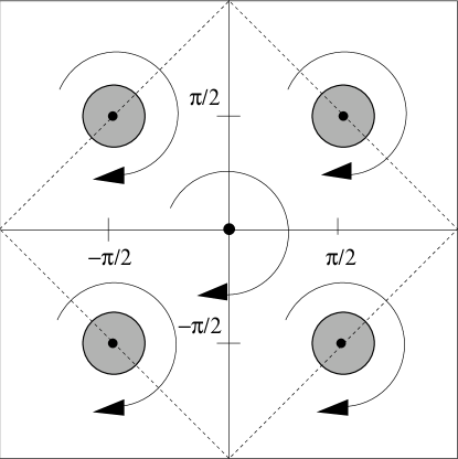
FIG. 1.: The structure of the pair wave function in momentum space: $\Delta({\bf k})$ is maximal around four Fermi points ${\bf k}_{f}=(\pm\frac{\pi}{2},\pm\frac{\pi}{2})$ and consists of four similarly oriented unit vortices around each Fermi point. The phase of each vortex is relative to the direction of the ${\bf k}_{f}$ as in the eq. (136). It changes sign under $90^{o}$ rotation $\Delta(-k_{y},k_{x})=-\Delta(k_{x},k_{y})$.

One of the motivations of this work was the corner-SQUID-junction experiment [4] in which the relative phase of tunneling amplitudes (3) on different faces of a single crystal of YBCO has been measured. It is found to be $\pi$ in accord with d-wave superconductivity and apparently in agreement with the topological mechanism (4).

These and many other anomalies in tunneling, transport, and the photoemission spectrum are due to a single phenomenon: the orthogonality catastrophe [5]. In a strongly interacting environment the addition of an extra particle to the system drastically changes its ground state. As a result the overlap between the ground states differing by an odd number of particles vanishes in the macroscopical system. Contrary ground states which differ by an even number of particles (3) are not orthogonal (compare to Ref.[6]).

Tunneling involves a correlation between particles with different spins. Another goal of this paper is to develop a method to treat the spin correlation.

This paper consists of four distinct parts. In Sec. II we discuss the Josephson tunneling in the presence of orthogonality catastrophe. Then, in Sec. III we give a phenomenological description of the topological mechanism of superconductivity. We describe hydrodynamics in Sec. III A and include Fermi surface in the consideration in Sec. III D. In Sec. III B we present a field theory model (44) which yields the phenomenological picture of Sec. III. We calculate tunneling amplitude and off-diagonal matrix elements for the incommensurate case in Secs. IV B,IV C and for the nearly half-filled (commensurate) case in Sec. V C. Finally, in the Appendix we describe a way to derive the model of topological superconductivity from a t-J model, a canonical model of correlated electronic systems. Although this section is of interest in its own right, we present it separately as an appendix for the sake of continuity of the text.

II Tunneling and orthogonality catastrophe

Josephson tunneling is peculiar in the presence of an orthogonality catastrophe. The Josephson current through the junction (at zero bias voltage) between two superconductors, of which one is conventional, is given by the well known formula [7]

$$I = -\,{\rm Im}\,i\sum_{kp}T_{kp}T_{-k-p}\frac{\Delta^{*}_{1}}{E_{k}}$$ (10)

$$\times \int_{0}^{\infty}\frac{d\omega}{2\pi}\left[\frac{F(p,\omega)}{\omega-E_{k}-i\eta}-\frac{F(p,-\omega)}{\omega-E_{k}+i\eta}\right],$$ (11)

where $T_{kp}$ is a transmission amplitude of the junction, $E_{k}=\sqrt{|\Delta_{1}|^{2}+\epsilon_{k}^{2}}$ is the spectrum of the conventional superconductor and $F(p,\omega)$ is the spectral function of the superconductor of interest

$$F(p,\omega)= 2\pi i\varepsilon^{\sigma\sigma^{\prime}}\sum\langle N|c_{\sigma}(p)|N+1\rangle$$ (12)

$$\times \langle N+1|c_{\sigma^{\prime}}(-p)|N+2\rangle\delta(\omega-\epsilon_{p}).$$ (13)

Here the sum goes over all quantum states with one extra particle ($\epsilon_{p}$ is the energy of an intermediate state). If the spectrum is symmetric with respect to adding or removing a particle, i.e., $F(p,\omega)$ is an odd function of $\omega$, we obtain

$$I=-2\,{\rm Im}\,i\sum_{kp}T_{kp}T_{-k-p}\frac{\Delta_{1}^{*}}{E_{k}}\int_{0}^{\infty}\,{\cal P}\frac{d\omega}{2\pi}\frac{F(p,\omega)}{\omega-E_{k}}.$$ (14)

In the following we assume for simplicity that the transmission amplitude $T_{kp}$ is strongly peaked at ${\bf k},\;{\bf p}$ close to the direction normal to the junction. This simplification should not change the phase dependence of the Josephson current although it can change the value of the critical current. Assuming that the gap in the superconductor of interest $\Delta_{0}$ is bigger than the one in the conventional superconductor $\Delta_{0}\gg\Delta_{1}$ we obtain:

$$I\sim|T|^{2}\nu_{0}|\Delta_{1}|\sum_{|{\bf p}_{n}|}\int_{0}^{\infty}\frac{d\omega}{\omega}\sin(\phi_{0}-\phi({{\bf p}_{n}},\omega))|F({\bf p}_{n},\omega)|,$$ (15)

where ${\bf p}_{n}$ is the component of momentum normal to the surface of the junction and averaging over ${\bf p}_{n}$ is determined by the actual form of the transition amplitude. In this formula $\phi_{0}$ and $\nu_{0}$ are the phase and density of states of the conventional superconductor and $\phi({\bf p},\omega)$ is the phase of the $F$-function (13) of the superconductor of interest.

In the BCS theory the $F$-function has a peak at the gap $\omega\sim\Delta_{0}$, such that the width of the peak is also of the order of the gap:

$$\int dpF_{\rm BCS}(p,\omega)\sim\frac{\Delta_{0}}{\sqrt{\omega^{2}-\Delta^{2}_{0}}}.$$ (16)

The peak gives the major contribution to the integral (15). It selects a characteristic energy of the intermediate state $\epsilon_{q}\sim\Delta_{0}$ and gives rise to the traditional BCS picture of tunneling: a pair decays into two electrons while tunneling, so electrons tunnel independently. Short time processes (at $\omega\sim\epsilon_{f}$) do not contribute to the integral (15).

The situation is drastically different in the orthogonality catastrophe environment [6]. We will show that in a topological superconductor an individual matrix element $\langle N|c_{\sigma}(p)|N+1\rangle$ acquires an additional factor $1/Lk_{f}$, where $L$ is the size of the system and therefore vanishes in a macroscopical sample, i.e., the ground states with $N$ and $N+1$ particles are almost orthogonal. Nevertheless, the tunneling, i.e., a matrix element between states with $N$ and $N+2$ particles is nonzero due to a large number of low-energy intermediate states contributing to the sum (13). A result of this is that the spectral function (13) acquires an additional factor $\omega/\epsilon_{f}$. In contrast to BCS at $\omega\gg\Delta_{0}$ we have

$$\int dpF(p,\omega)\sim\frac{\Delta_{0}}{\omega}\left(\frac{\omega}{\epsilon_{f}}\right)\sim\frac{\Delta_{0}}{\epsilon_{f}}.$$ (17)

Therefore, the characteristic scale of spectral function is shifted to the ultraviolet and becomes of the order of the Fermi energy—much larger than the scale of the gap [A similar phenomenon occurs in momentum space. In the Sec. IV C we show that the pair wave function $\Delta(k)$ has a long tail well away from the Fermi surface (see also Fig. 2)]: the integral (15) is saturated by $\omega\sim\epsilon_{f}\gg\Delta_{0}$. This means that a pair remains intact during the tunneling and the tunneling amplitude is determined by the equal time value of $F(p,t=0)$, i.e., by the matrix element $\Delta({\bf r})$ of an instantaneous creation of a pair (3). Let us notice that the correction to the spectral function in the eq. (17)—$(\omega/\epsilon_{f})^{\alpha}$ at $\alpha=1$ is just marginal. Were $\alpha$ be less than 1 the time of the tunneling would be of the order of $\Delta_{0}^{-1}$ (A similar phenomenon has been discussed by Chakravarty and Anderson in the context of interlayer tunneling in cuprate superconductors [6]).

In the coordinate representation the Josephson current is

$$I\sim\,{\rm Im}\,e^{-i\phi_{o}}\Delta({k_{f}{\bf n}})\sim\sin(\phi_{0}-\phi(k_{f}{\bf n},\omega=0)).$$ (18)

In the corner-SQUID-junction geometry [8, 4] one can directly measure the difference of phases of $\Delta$ between two faces of the superconducting crystal.

The instantaneous character of tunneling and the power laws (17) are known from one-dimensional electronic systems where the orthogonality catastrophe comes to its own. In addition, in 2D it also leads to the angular dependence of the two-particle amplitude (3,5).

The direct tunneling current is also strongly affected by the orthogonality catastrophe:

$$I_{\rm dir}=2|T|^{2}\nu_{0}\int_{0}^{eV}\frac{d\omega}{2\pi}\int\frac{d{\bf k}}{(2\pi)^{2}}\,{\rm Im}\,G(\omega,{\bf k}).$$ (19)

Elsewhere we will show that due to the orthogonality catastrophe the one-particle Green function acquires a branch cut, rather than a pole on the threshold. As a result the density of states in a topological superconductor just above the gap is suppressed by the factor $\sqrt{\omega-\Delta_{0}}$. This leads to a suppression of direct current close to the threshold bias voltage. With a logarithmic accuracy we will obtain almost linear I-V behavior

$$I_{\rm dir}\sim(V-\Delta_{0}).$$ (20)

This is to be compared to the BCS-theory result: $I_{\rm dir}\sim(V-\Delta_{0})^{1/2}$.

III Topological Mechanism of Superconductivity

A Hydrodynamics

The mechanism of topological superconductivity is a generalization to higher dimensions of the Peierls-Fröhlich phenomenon, known from one-dimensional electron-phonon systems [9, 10, 11, 12, 13, 14]. It inherits major features from electronic physics in one dimension. We attempt to present it here without addressing a particular model but accepting some minimal assumptions. Later in the Appendix we develop a microscopical model to justify and illustrate the phenomenological picture.

(i) Zero Modes and Topological Instability. Let us consider an electronic liquid where the interaction between electrons is mediated by an electrically neutral bosonic field, that can form a point-like spatial topological configuration (soliton). Let us suppose, that in a sector with zero topological charge the electronic spectrum has a gap $m$. Assume now that in the presence of a static soliton the electronic spectrum differs from an unperturbed one by an additional state just at the top of the valence band or within the gap—a so-called zero mode or a midgap state [15]. If the zero mode is separated from the spectrum, its wave function is localized around the core of the topological defect. In case when the level is attached to a band, the wave function decays as a power law away from the center of the soliton. A general argument [16] suggests that the midgap state always has an even degeneracy. This degeneracy leads eventually to a proper flux quantization and below it is assumed to be twofold.

Now let us add an even number of extra electrons with a concentration $\delta$ into the system. They may occupy a new state at the Fermi level of the conduction band. It costs the energy of the gap plus the Fermi energy $m+\mu_{f}$ per particle, where $\mu_{f}$ is a chemical potential. Alternatively, the system may create a topological configuration and a number of zero modes in order to accommodate all extra particles. The energy of this state is the soliton mass plus exponentially small corrections due to the interactions between zero modes. If the latter energy is less than $\mu_{f}$ then every two extra electrons added to the system create a soliton and then completely fill a zero mode, rather than occupy the Fermi level of the state with zero topological charge. As a result the total number of solitons in the ground state is equal to half of the total number of electrons in the system.

Formally it means that, contrary to the Landau Fermi-liquid picture, the expansion of the energy in small smooth variation of chemical potential $\delta\mu({\bf r})$ has a non vanishing linear term in $\delta\mu$:

$$\delta E(\mu)= \int \delta\mu({\bf r}){\bar{\rho}}\,d{\bf r}+\int\delta\mu({\bf r})K(\mu,{\bf r}-{\bf r}^{\prime})\frac{F({\bf r}^{\prime})}{2\pi}\,d{\bf r}d{\bf r}^{\prime}$$ (21)

$$+ {\cal O}(\delta\mu^{2}).$$ (22)

Here ${\bar{\rho}}$ is the electronic density, $F({\bf r})/2\pi$ is a density of a topological charge and $K(\mu,{\bf r})$ is some kernel. The linear term in chemical potential is known as Chern-Simons term.

The minimum of energy is achieved if the variation of density is followed by the variation of the topological charge

$$\rho({\bf r})-\bar{\rho}=\int K(\mu,{\bf r}-{\bf r}^{\prime})\frac{F({\bf r}^{\prime})}{2\pi}d{\bf r^{\prime}}.$$ (23)

While doping, electrons create and occupy zero mode states to minimize their energy, thus giving a non zero value to the topological charge. Due to the twofold degeneracy of zero mode states

$$\int K(\mu,{\bf r})\,d{\bf r}=2$$ (24)

so a number of extra particles $\delta$ gives rise to a flux

$$\delta=2\int\frac{F({\bf r})}{2\pi}d{\bf r}.$$ (25)

We refer to this phenomenon as topological instability. Once zero mode states are occupied, residual interaction between them lifts the degeneracy, so that zero mode states form a narrow band. This band is always completely filled and is detached from the rest of the spectrum by some gap $\Delta_{0}$.

This is already sufficient to conclude about superconductivity — the chemical potential always lies in a gap. The following arguments are borrowed from Fröhlich’s paper [9]. The position of the topological excitation is not fixed relative to the crystal lattice. Therefore, a pair of electrons bound to a topological excitation can easily slide through the system (and therefore carry electric current). It slides unattenuatedly, since the state is completely filled and is separated by the gap from the unoccupied electronic states. As a result, the low energy physics of density fluctuations is described by the hydrodynamics of a liquid of zero modes:

$$H=\frac{1}{2\bar{\rho}}[v_{0}^{2}(\rho-\bar{\rho})^{2}+{\bf j}^{2}]$$ (26)

where $\bar{\rho},\,v_{0}$ are the average density and the velocity of the sound mode, ${\bf j}=\rho{\bf v}$ is the current and ${\bf v}$ is the velocity

$$[\rho({\bf r}),{\bf v}({\bf r}^{\prime})]=-i\mbox{\boldmath$\nabla$}_{r}\delta({\bf r}-{\bf r}^{\prime}).$$ (27)

In dimensions higher than one, where the pinning effects are not that important, the eqs. (26,27) already imply the Meissner effect (1) and superconductivity [13, 14].

It is convenient to re-parameterize densities and currents in terms of charge displacement ${\bf u}$:

$$\rho-\bar{\rho}=-\mbox{\boldmath$\nabla$}{\bf u},\;\;\;{\bf j}=\partial_{t}{\bf u},$$ (28)

so that

$$[j_{i}({\bf r}),u_{k}({\bf r}^{\prime})]=-i\bar{\rho}\delta_{ik}\delta({\bf r}-{\bf r}^{\prime}).$$ (29)

Let us stress that this mechanism is very different from the mechanism where an electronic pair is localized by a polaron. In contrast, in the topological mechanism the electric charge of a pair is only partially localized at the core of the topological soliton. Although the number of zero modes is equal to the topological charge of the soliton, a part of the charge is smoothly distributed throughout the rest of the system.

(ii) Single-valuedness and gauge invariance. The electronic wave function is single-valued. This important property may be reformulated in terms of gauge invariance. In two spatial dimensions a topological density can be described by means of a gauge field ${\bf A}$:

$$F({\bf r})=\mbox{\boldmath$\nabla$}\times{\bf A}.$$ (30)

The single-valuedness of the electronic wave function means that electrons are neutral with respect to this field: the electronic operator does not transform under the gauge transformation ${\bf A}\rightarrow{\bf A}+\mbox{\boldmath$\nabla$}\Lambda$, i.e.,

$$[A_{i}({\bf r}),u_{k}({\bf r}^{\prime})]=0;\;\;\;[A_{i}({\bf r}),j_{k}({\bf r}^{\prime})]=0.$$ (31)

Let us note that, despite of what eq. (23) suggests, the vector potential $A_{i}$ is not equal to the displacement $\varepsilon^{ik}u_{k}$ but differs from it by a singular gauge transformation.

In fact the wave functions of zero modes represent conformal blocks of some conformal field theory.

(iii) Incompressible chiral spin liquid. The hydrodynamics of charge degrees of freedom alone is not sufficient to draw conclusions about fermionic matrix elements. They are determined also by the distribution of electronic spin within the zero mode. Unless there are solitons which create zero modes in spin sector, the compressibility with respect to density modulations generally results in incompressibility with respect to spin modulations. Moreover, the spin liquid in the singlet sector is a topological liquid. In the next section we show that on a very general basis, spin displacements ${\bf u}_{s}$ defined as $S^{3}=-1/2\mbox{\boldmath$\nabla$}{\bf u}_{s}$ obey anomalous commutation relations

$$\left[{\bf u}_{s}({\bf r})\times{\bf u}_{s}({\bf r}^{\prime})\right]=2i\pi\delta({\bf r}-{\bf r}^{\prime})$$ (32)

in addition to standard $[j_{i,s}({\bf r}),u_{k,s}({\bf r}^{\prime})]=-i\bar{\rho}\delta_{ik}\delta({\bf r}-{\bf r}^{\prime})$. This property determines rotational properties of a local singlet—it has $l=2$ angular momentum—and eventually determines the phase of the tunneling amplitude (4).

By combining charge and spin parts of the hydrodynamics (26, 32) we obtain the hydrodynamics of topological superconductivity:

$${\cal L} = {\cal L}_{c}+{\cal L}_{s},$$ (33)

$${\cal L}_{c} = \frac{1}{2\bar{\rho}}((\partial_{t}{\bf u})^{2}-v_{0}^{2}(\mbox{\boldmath$\nabla$}{\bf u})^{2}),$$ (34)

$${\cal L}_{s} = 2\pi{\bf u}_{s}\times\partial_{t}{\bf u}_{s}+\frac{1}{2\bar{\rho}}((\partial_{t}{\bf u}_{s})^{2}-v_{0}^{2}(\mbox{\boldmath$\nabla$}{\bf u}_{s})^{2}).$$ (35)

The hydrodynamics consists of two independent fluids: a compressible charged liquid

$$\langle u^{\parallel}(\omega,{\bf k}),u^{\parallel}(-\omega,-{\bf k})\rangle = \frac{\bar{\rho}}{\omega^{2}-(v_{0}{\bf k})^{2}},$$ (36)

$$\langle u^{\perp}(\omega,{\bf k}),u^{\perp}(-\omega,-{\bf k})\rangle = \frac{\bar{\rho}}{\omega^{2}},$$ (37)

and an incompressible topological (chiral) spin liquid

$$\langle u^{\parallel}_{s}(\omega,{\bf k}),u^{\parallel}_{s}(-\omega,-{\bf k})\rangle = -\frac{1}{\vartheta^{2}\bar{\rho}},$$ (38)

$$\langle u^{\perp}_{s}(\omega,{\bf k}),u^{\perp}_{s}(-\omega,-{\bf k})\rangle = -\frac{1}{\vartheta^{2}\bar{\rho}}(1-\frac{v_{0}^{2}{\bf k}^{2}}{\omega^{2}}),$$ (39)

$$\langle u^{\parallel}_{s}(\omega,{\bf k}),u^{\perp}_{s}(-\omega,-{\bf k})\rangle = \frac{i}{\vartheta\omega},$$ (40)

where $\vartheta=4\pi$ and $u^{\parallel}$, $u^{\perp}$ are the longitudinal and transversal parts of the displacement $u_{i}({\bf k})=\frac{k_{i}}{k}u^{\parallel}+\frac{\varepsilon^{ij}k_{j}}{k}u^{\perp}$. Eqs. (36) imply compressibility of the charge fluid and the Meissner effect. The absence of the sound mode in the spin liquid (39) is the consequence of the topological mass generated by the Chern-Simons term in (35).

(iv) Edge Spin Current. One of the direct consequences of the chiral nature of the spin liquid is that the spin liquid generates spin edge current. Indeed, the spin sector of the hydrodynamics (35) is equivalent to the hydrodynamics of the FQHE fluid (see e.g., [17, 18]). Similar to the FQHE the spin excitations are suppressed in the bulk but develop a spontaneous spin edge current with the level $k=2$ current algebra. Let us stress that the spin edge current is the only hydrodynamical manifestation of spontaneous parity breaking. Contrary to a number of claims scattered through the literature, the spontaneous parity breaking is invisible in the charge sector even for the systems with an odd number of layers.

B The field theory

Let us realize the commutation relation (27,29,31,32) by means of an electron operator:

$$\rho = c^{\dagger}c;\;\;\;\;\;\;{\bf j}=-ic^{\dagger}\mbox{\boldmath$\nabla$}c;$$ (41)

$$S^{3} = \frac{1}{2}c^{\dagger}\sigma^{3}c;\;\;\;\;{\bf j}_{s}=-\frac{1}{2}ic^{\dagger}\sigma^{3}\mbox{\boldmath$\nabla$}c.$$ (42)

The topological constraint (25) reduces the Hilbert space of the low-energy sector of the theory. Instead of using a projected electronic operator $c_{\sigma}$ we introduce a ”spinned“ fermion operator $\psi_{\sigma}$ in which terms the field theory which takes topological constraint (25) into account is local. We discuss the relation between the physical electron operator $c_{\sigma}$ and the unphysical gauge non-invariant operator $\psi_{\sigma}$ in the Secs. III D,IV A. In $\psi$ representation the density of electrons is

$$\rho=\sum_{\sigma}c^{\dagger}_{\sigma}c_{\sigma}=\sum_{\sigma}\psi^{\dagger}_{\sigma}\psi_{\sigma}.$$ (43)

A standard example of the theory which exhibits the topological instability and therefore superconductivity is the Dirac Hamiltonian

$$H=\psi^{\dagger}_{\sigma}\mbox{\boldmath$\alpha$}\big{(}-i\mbox{\boldmath$\nabla$}+{\bf A}\big{)}\psi_{\sigma}+\Delta_{0}\psi^{\dagger}_{\sigma}\beta\psi_{\sigma}-\mu\psi^{\dagger}_{\sigma}\psi_{\sigma}.$$ (44)

where $\mbox{\boldmath$\alpha$}=(\alpha_{x},\alpha_{y})$ and $\beta$ are $2\times 2$ Dirac matrices: $\{\alpha_{x},\alpha_{y}\}=0,\;\beta=-i\alpha_{x}\alpha_{y}$. This Hamiltonian has $\frac{2}{2\pi}\int F({\bf r})d{\bf r}$ zero modes (the flux is directed up). Wave functions of zero modes are:

$$\Phi({\bf r}) = e^{-i\int^{\bf r}{\bf A}({\bf r}^{\prime})\cdot d{\bf r}^{\prime}-\beta\int^{\bf r}{\bf A}({\bf r}^{\prime})\times d{\bf r}^{\prime}}\Phi_{0}({\bar{z}}),$$ (45)

$$\beta\Phi_{0}({\bar{z}}) = -\Phi_{0}({\bar{z}})$$ (46)

where $\Phi_{0}$ is any polynomial of degree $\frac{1}{2\pi}\int F({\bf r})d{\bf r}-1$ [20]. The fact of existence of zero modes implies that the energy at $\mu=0$ has a linear term (22) in chemical potential $K(\mu=0,{\bf r})=2\delta({\bf r})$. Other models of topological superconductivity were discussed in Refs.[13, 14].

Let us comment on the relation between topological mechanism of superconductivity and superconductivity in the system of anyons [11, 12]. The models become very close after projection onto the low energy sector, where the relation (23) is treated as a constraint rather than as a result of minimization of the energy. The projection can be done by introducing a Lagrangian multiplier $A_{0}$ for the relation (23) and commutation relations $\left[A_{x}({\bf r}),A_{y}({\bf r}^{\prime})\right]=2\pi iK^{-1}({\bf r}-{\bf r}^{\prime})$, i.e. by adding the Chern-Simons term with the kernel $K$ to the Lagrangian. In anyon model the kernel $K({\bf r})$ is replaced by $2\delta({\bf r})$ (even at $\mu\neq 0$), so that the relation between topological charge and the density becomes local $\rho({\bf r})=2\frac{F({\bf r})}{2\pi}$. This simplification results in a generation of transversal electric currents or ”internal“ magnetic field by light or by inhomogeneous electric charge. Due to the same reason, the Meissner effect in the anyon model per se exists only at zero frequency, zero momentum, zero temperature, infinitesimal magnetic field etc. These unphysical consequences originate from the topological constraint (25). To avoid them one must determine the kernel $K(\mu,{\bf r})$ self-consistently.

The topological mechanism of superconductivity takes place in certain models of 2D doped Mott insulators. We point out several steps involved in the derivation of the Dirac Hamiltonian (44) in Appendix, while here we would like to give a physical interpretation of the vector potential ${\bf A}$ and its flux ${\bf F}$. The vector potential $A_{i}$ is the phase of the hopping amplitude of an electron in direction $i=x,y$. Its flux is the phase of the total hopping amplitude along a closed path. On a square lattice at small doping it is

$$F({\bf r})=-\,{\rm Im}\,\ln\,\mbox{tr}\,{\bf W},$$ (47)

where the chirality ${\bf W}$ is defined as

$${\bf W} = (\frac{1}{2}+\mbox{\boldmath$\sigma$}\cdot{\bf S}({\bf r}))(\frac{1}{2}+\mbox{\boldmath$\sigma$}\cdot{\bf S}({\bf r}+{\bf e}_{x}))$$ (48)

$$\times (\frac{1}{2}+\mbox{\boldmath$\sigma$}\cdot{\bf S}({\bf r}+{\bf e}_{y}+{\bf e}_{x}))$$ (49)

and ${\bf r},{\bf r}+{\bf e}_{x},{\bf r}+{\bf e}_{x}+{\bf e}_{y}$ are three consecutive points of a lattice and $\sigma$ are auxiliary Pauli matrices.

C Hydrodynamics from the mean-field approximation

The hydrodynamics of a superfluid (34) can easily be obtained from the model (44). Let us see how the energy (22) of a spin singlet state changes under smooth variations of “electric” ${\bf E}=\partial_{t}{\bf A}-\mbox{\boldmath$\nabla$}\delta\mu$ and “magnetic” $F=\mbox{\boldmath$\nabla$}\times{\bf A}$ fields. To keep track of spin variations we add an external field ${\bf{\cal A}}^{3}$ to the Hamiltonian (44) $i\mbox{\boldmath$\nabla$}-{\bf A}\rightarrow i\mbox{\boldmath$\nabla$}-{\bf A}-{\bf{\cal A}}^{3}\sigma_{3}$. In Gaussian approximation the result consists of two separate parts—spin and charge. In the Coulomb gauge $\mbox{\boldmath$\nabla$}{\bf A}=0$ the density of energy is

$$\delta E = \delta E_{c}+\delta E_{s},$$ (50)

$$\delta E_{c} = \frac{\Pi_{0}}{2}{\bf E}^{2}+\frac{\Pi_{\perp}}{2}F^{2}+\delta\mu\big{(}\frac{K}{2\pi}\mbox{\boldmath$\nabla$}\times{\bf a}-\delta{\rho}\big{)},$$ (51)

$$\delta E_{s} = \frac{\Pi_{0}}{2}(\partial_{t}{\bf{\cal A}}^{3})^{2}+\frac{\Pi_{\perp}}{2}(\mbox{\boldmath$\nabla$}\times{\bf{\cal A}}^{3})^{2}+\frac{K}{2\pi}{\bf{\cal A}}^{3}\times\partial_{t}{\bf{\cal A}}^{3},$$ (52)

where polarization operators

$$\Pi_{0} = \omega^{-2}\langle j_{\parallel}(\omega,{\bf k})j_{\parallel}(-\omega,-{\bf k})\rangle,$$ (53)

$$\Pi_{\perp} = k^{-2}\langle j_{\perp}(\omega,{\bf k})j_{\perp}(-\omega,-{\bf k})-j_{\parallel}(\omega,{\bf k})j_{\parallel}(-\omega,-{\bf k})\rangle,$$ (54)

$$K = i\omega^{-1}\langle j_{\parallel}(\omega,{\bf k})j_{\perp}(-\omega,-{\bf k}\rangle$$ (55)

are transversal current-current correlators of free Dirac massive fermions at ${\bf k},\omega\rightarrow 0$. Since the particles are massive the propagators (55) are known to be $\Pi_{0}=\Pi_{\perp}v_{0}^{-2}\rightarrow\mbox{const}$ and $K\rightarrow 2$ .

To obtain the hydrodynamics (33) one must rewrite this result in terms of spin and charge displacements. Minimization over $\delta\mu$ gives the relation (23) for the charge sector. Substituting this relation into (51) gives the hydrodynamics of the ideal liquid (34). In the spin sector (52) the story is different. The total spin is kept to be zero. Therefore, the Chern-Simons term remains in the spin sector and gives the hydrodynamics of an incompressible spin liquid. Writing $\partial_{t}{\bf u}_{s}=-\delta{\cal L}/\delta{\bf{\cal A}}^{3}$, we obtain the eq. (35).

D Electron as a composite object. The vertex operator

The most difficult part of the theory is to find a relation between the true electron operator $c_{\sigma}$ and “spinned” fermion $\psi_{\sigma}$. The problem is that the local field theory (44), is written in terms of a not gauge invariant operator $\psi_{\sigma}$. Moreover, without gauge field (i.e. without interaction) $\psi_{\sigma}$ being a Dirac spinor has 1/2 - orbital momentum. The electronic states are gauge invariant, and spin singlet states must have an integer orbital momentum. Another problem is that an electronic excitation carries a typical momentum of the order of $k_{f}$, while typical momenta of Dirac particles are close to zero. These difficulties do not occur while studying the hydrodynamics, but rise in matrix elements. Below we employ two approaches. In Appendix we derive the Dirac theory (44) from a microscopical model of a doped Mott insulator and find the electronic operator and the vertex operator on a regular basis. In this section we conjecture the form of the electronic operator based on plausible physical arguments.

The requirements for the electronic states are
(i) electron is gauge invariant, i.e. remains unchanged under a non-singular gradient transformation ${\bf A}\rightarrow{\bf A}+\mbox{\boldmath$\nabla$}\Lambda$;
(ii) In a sector with completely filled zero modes, i.e. the flux and the number of particles obey the topological constraint (25), a charged singlet excitation is a spatial scalar, i.e. its wave function has a zero orbital moment $l=0$;
(iii) Since an electronic liquid is compressible, the most essential electronic modes have momenta $k\sim(2\pi/{\bar{\rho}})^{1/2}\equiv k_{f}$.

We find the electronic operator in three steps. First we take care of the gauge invariance. We define the vertex operator $V_{\sigma}({\bf r})$ as an operator which creates a flux quantum and a zero mode at the point ${\bf r}$ in the state with the spin $\sigma=\pm 1/2$[19]. It obeys two relations

$$V_{\sigma}^{-1}\mbox{\boldmath$\alpha$}(-i\mbox{\boldmath$\nabla$}+{\bf A})V_{\sigma}=-i\mbox{\boldmath$\alpha$}\mbox{\boldmath$\nabla$},$$ (56)

$$\,[F({\bf r}^{\prime}),V_{\sigma}({\bf r})]=2\pi V_{\sigma}({\bf r})\delta({\bf r}-{\bf r}^{\prime}).$$ (57)

These conditions are valid in the subspace of zero modes (45) and can be solved by virtue of the commutation relations of the Chern-Simons theory $\left[A_{x}({\bf r}),A_{y}({\bf r}^{\prime})\right]=i\pi\delta({\bf r}-{\bf r}^{\prime})$. In terms of the density of particles with spin $\sigma$: $c_{\sigma}^{\dagger}c_{\sigma}=-\mbox{\boldmath$\nabla$}\cdot{\bf u}_{\sigma}$, or in terms of their displacements ${\bf u}_{\sigma}$ the vertex operator can be written as

$$V_{\sigma}({\bf r})=e^{2\pi i\int^{\bf r}{\bf u}_{\sigma}({\bf r}^{\prime})\times d{\bf r}^{\prime}-2\pi\beta\int^{\bf r}{\bf u}_{\sigma}({\bf r}^{\prime})\cdot d{\bf r}^{\prime}}.$$ (58)

The operator $V^{-1}_{\sigma}\psi_{\sigma}$ is gauge invariant.

The second step is the rotational invariance. Let us consider a wave function of the free Dirac field in two spatial dimensions. In the basis, where $\alpha$-matrices are $\alpha_{x}=\sigma_{3},\,\alpha_{y}=-\sigma_{2},\,\beta=\sigma_{1}$, the solution of the Dirac equation with momentum ${\bf p}$ is $e^{i{\bf p}{\bf r}}e^{-\frac{i}{2}\beta{\rm arg}(\bf p)}(u_{p},\,v_{p})$ for the positive energy $E=+E_{p}=\sqrt{p^{2}+\Delta_{0}^{2}}$, and $e^{i{\bf p}{\bf r}}e^{-\frac{i}{2}\beta{\rm arg}(\bf p)}(v_{p},-u_{p})$ for $E=-E_{p}$ , where ${\rm arg}(\bf p)$ is an angle of the momentum ${\bf p}$, relative to the x-axis and $u_{p}=\sqrt{\frac{1}{2}(1+\frac{|{\bf p}|}{E_{p}})}$ and $v_{p}=\sqrt{\frac{1}{2}(1-\frac{|{\bf p}|}{E_{p}})}$ are the BCS wave functions. The spinor carries an angular momentum $l=1/2$. We unwind the Dirac field by a chiral rotation

$$\psi_{\sigma}({\bf p})\rightarrow e^{\frac{i}{2}\beta{\rm arg}(\bf p)}\psi_{\sigma}({\bf p}).$$ (59)

This singular transformation has a clear physical sense—it projects the spinor wave function onto a direction of the momentum ${\bf p}$. Indeed, the chiral transformation (59) in two spatial dimensions, where $\beta=-i/2\left[\alpha_{x},\,\alpha_{y}\right]$ is equivalent to a spatial rotation of the momentum ${\bf p}$ by the angle ${\rm arg}(\bf p)$ which aligns the momentum ${\bf p}$ along the x-axis of the coordinate system. Now, without topological gauge fluctuations, the transformed operator is a spatial scalar.

The third step is to boost the fermion to the Fermi surface. In the chosen basis the upper and the lower components of the Dirac field $\psi_{\sigma}=\Big{(}\psi_{\sigma}^{(1)},\,\psi_{\sigma}^{(2)}\Big{)}$ correspond to the states propagating forward and backward along the vector ${\bf p}$. To construct an electronic operator we shift the momentum of the upper component by the Fermi vector ${\bf k_{f}}=k_{f}\frac{{\bf p}}{p}$ directed along the momentum ${\bf p}$: ${\bf p}\rightarrow{\bf k}\equiv{\bf k_{f}}+{\bf p}$ and the momentum of the lower component by $-{\bf k_{f}}$: ${\bf p}\rightarrow{\bf k}-2{\bf k_{f}}=-{\bf k_{f}}+{\bf p}$

$$\left(\begin{array}[]{c}\tilde{c}_{\sigma}({\bf k_{f}}+{\bf p})\\ \tilde{c}_{\sigma}(-{\bf k_{f}}+{\bf p})\end{array}\right)\sim e^{\frac{i}{2}\beta{\rm arg}(\bf k)}\psi_{\sigma}({\bf p}).$$ (60)

Here we used $\tilde{c}_{\sigma}$ to indicate that the gauge field has not been taken into account yet.

Formally, the chiral rotation (59) may be also understood in the following way. The wave function of the Dirac field depends explicitly on the choice of $\alpha$-matrices, i.e. on the choice of holomorphic coordinates in a plane. The chiral transformation aligns holomorphic coordinates relative to each point of the “Fermi surface”, i.e. sets up the momentum dependent $\alpha$-matrices

$$\mbox{\boldmath$\alpha$}_{\bf k_{f}}=e^{\frac{i}{2}\beta{\rm arg}({\bf k_{f}})}\mbox{\boldmath$\alpha$}e^{-\frac{i}{2}\beta{\rm arg}({\bf k_{f}})}.$$

In terms of $\tilde{c}$ the free Dirac Hamiltonian describes isotropic backward scattering

$$H=\int\left\{\xi_{k}\tilde{c}^{\dagger}_{\sigma}({\bf k})\tilde{c}({\bf k})+\Delta_{0}\,\Big{(}\tilde{c}^{\dagger}({\bf k})\tilde{c}({\bf k}-2{\bf k_{f}})+h.c.\Big{)}\right\}\,d{\bf k},$$ (61)

where $\xi_{k}=v(k-k_{f})$.

Assembling all pieces we obtain the relation between the Dirac fermion and the physical electron in the sector of zero modes

$$V_{\sigma}({\bf r})c_{\sigma}({\bf r})\sim\;\int e^{-i{\bf k}{\bf r}}e^{-\frac{i}{2}{\rm arg}({\bf k})}\psi_{\sigma}^{(\beta=-1)}({\bf k}-{\bf k_{f}})\,d{\bf k}$$ (62)

where $\psi_{\sigma}^{(\beta=-1)}$ is the Dirac field, projected onto the zero mode sector ( $\frac{1-\beta}{2}\psi_{\sigma}=\left(\begin{array}[]{c}1\\ -1\end{array}\right)\psi_{\sigma}^{(\beta=-1)}$).

IV Matrix Elements in Topological Liquids

A Vertex operators

To compute matrix elements we will need an operator algebra for the vertex operator $V_{\sigma}$ and two additional vertex operators of the charge and spin sectors $V=(V_{\uparrow})^{1/2}(V_{\downarrow})^{1/2}$ and $V_{s}=(V_{\uparrow})^{1/2}(V_{\downarrow})^{-1/2}$. Below we choose a holomorphic basis where $\beta=\sigma_{3}$ is diagonal. At $\beta=-1$ (the flux up) the vertex operators depend on the holomorphic part of the displacement $u_{\sigma}=u_{\sigma,x}+u_{\sigma,y}$:

$$V(w) \sim e^{i\pi\int^{w}u(z)dz},$$ (63)

$$V_{s}(w) \sim e^{i\pi\int^{w}u_{s}(z)dz},$$ (64)

where $u=(u_{\uparrow}+u_{\downarrow})/2;\;\;u_{s}=(u_{\uparrow}-u_{\downarrow})/2$. Due to the commutation relations (32) vertex operators obey the operator algebra:

$$V_{s}(z)c_{\uparrow}(z^{\prime}) \sim (\frac{z-z^{\prime}}{L})^{1/2}c_{\uparrow}(z^{\prime})V_{s}(z),$$ (65)

$$V_{s}(z)c_{\downarrow}(z^{\prime}) \sim (\frac{z-z^{\prime}}{L})^{-1/2}c_{\downarrow}(z^{\prime})V_{s}(z),$$ (66)

$$V(z)c_{\sigma}(z^{\prime}) \sim (\frac{z-z^{\prime}}{L})^{1/2}c_{\sigma}(z^{\prime})V(z),$$ (67)

$$V(z)V_{s}(z^{\prime}) \sim V_{s}(z^{\prime})V(z),$$ (68)

$$V(z)V(z^{\prime}) \sim V(z^{\prime})V(z).$$ (69)

Below we also use a two-particle vertex operator $\mu(u,w)$ which creates a soliton and antisoliton of the spin displacement

$$\mu(u,w)=V_{s}(u)V_{s}^{-1}(w).$$ (70)

The operator algebra gives

$$\mu(u^{\prime},w^{\prime})c_{\uparrow}^{\dagger}(u)c_{\downarrow}^{\dagger}(w) = \frac{(u^{\prime}-u)^{1/2}(w^{\prime}-w)^{1/2}}{(u-w)}$$ (71)

$$\times c_{\uparrow}^{\dagger}(u)c_{\downarrow}^{\dagger}(w)\mu(u^{\prime},w^{\prime})$$ (72)

and if the points $u,u^{\prime}$ and $w,w^{\prime}$ coincide

$$c_{\uparrow}(u)c_{\downarrow}(w)\mu(u,w)\sim\frac{a}{(u-w)}\mu(u,w)c_{\uparrow}(u)c_{\downarrow}(w).$$ (73)

The physical meaning of the vertex operators is straightforward. The vertex operator of the spin sector $V_{s}(z)$ creates a soliton of the spin displacement ${\bf u}_{s}$ and removes spin up from the site $z$. Indeed due to (32), we have

$$\left[V_{s}(z),{\bf\nabla}{\bf u}_{s}(z^{\prime})\right]=V_{s}(z)\delta(z-z^{\prime}).$$ (74)

In contrast, the vertex operator of the charge channel $V(z)$ creates a flux of the gauge field (the spin chirality), but commutes with displacements

$$[F(w),V(z)] = 2\pi V(z)\delta(w-z),$$ (75)

$$\mbox{}[u(w),V(z)] = 0.$$ (76)

Two composite objects $V_{s}(z)c_{\uparrow}(z)$ and $V_{s}(z)c_{\downarrow}(z)$ are singlets but carry electric charge.

B Matrix elements

An electronic operator $c_{\sigma}$ does not create an elementary excitation. The ground state with an extra particle is created by a composite operator which creates a flux and places a particle into the core of the flux. Creating a flux also generates spin waves. They are gapful. Let us first assume that the gap $\Delta_{0}$ is very large and we can neglect spin excitations. Then the vertex operator $V$ of the charge sector creates a flux and a zero mode which gets occupied by a particle created by the operator ${\psi_{\sigma}^{(\beta=-1)}}^{\dagger}$.

Let us start from the two-particle state with zero momentum:

$$|N+2\rangle \sim \varepsilon_{\sigma\sigma^{\prime}}\int d{\bf r}\,d{\bf r}^{\prime}$$ (77)

$$\times V({\bf r})V({\bf r}^{\prime}){\psi_{\sigma}^{(\beta=-1)}}^{\dagger}({\bf r}){\psi_{\sigma^{\prime}}^{(\beta=-1)}}^{\dagger}({\bf r^{\prime}})|N\rangle.$$ (78)

A physical meaning of the composite operator which creates the ground state with an extra particle is more transparent in terms of gauge invariant electronic operators $c_{\sigma}\sim V_{\sigma}^{-1}\psi_{\sigma}^{(\beta=-1)}$. In these terms the operators $V^{-1}\psi_{\uparrow}^{(\beta=-1)}\sim V_{s}c_{\uparrow}$ and $V^{-1}\psi_{\downarrow}^{(\beta=-1)}\sim V_{s}^{-1}c_{\downarrow}$ consist of the electron and the vortex (antivortex) of the spin density only. In its turn, the two-particle state (77) is composed of the two electrons and the operator (70), creating a vortex and an antivortex of spin density at the points of electron insertions. Electrons with opposite spins see each other with vortices of the opposite angular momenta $l=\pm 1$ (compare to Ref. [21]). This gives an angular momentum $l=2$ for the pair.

With the help of the operator algebra (66,72,73) we are able to compute the tunneling amplitude as well as some other matrix elements.

The singlet two-particle matrix element $\Delta({\bf r})=\langle N|c_{\uparrow}({\bf r})c_{\downarrow}(0)|N+2\rangle$ has the form

$$\Delta({\bf r})\sim\int d{\bf k}\,e^{-i\arg({\bf k})}e^{i{\bf k}{\bf r}}$$ (79)

$$\times\langle N+2|V_{s}({\bf r})V^{-1}_{s}(0)|N+2\rangle.$$ (80)

Thus the two-particle matrix element is given by the correlation function of the vertex operators of the spin channel. The operator algebra $V_{s}(z)V_{s}^{-1}(z^{\prime})=\frac{a}{z-z^{\prime}}:V_{s}(z)V_{s}^{-1}(z^{\prime}):$ implies $\langle N+2|V_{s}({\bf r})V^{-1}_{s}(0)|N+2\rangle\sim\frac{1}{k_{f}r}e^{-i\arg({\bf r})}$, so that

$$\Delta({\bf r})\sim\frac{1}{k_{f}r}e^{-i\arg({\bf r})}\int e^{-i\arg({\bf k})}e^{i{\bf k}{\bf r}}d{\bf k}$$ (81)

The matrix element (81) is obtained in the limit of a very large gap $\Delta_{0}\rightarrow\infty$. This approximation is sufficient in order to analyze the transformation properties and the angular dependence of the tunneling amplitude. If the gap is not very large, an embedding of two extra particles creates a gapful spinon-antispinon excitations. These excitations do not interact with the zero mode of the charged sector and their wave functions (at ${\bf kr}\gg 1$) are just the wave functions of an unperturbed theory (61)

$$\Phi^{(+)}({\bf k},{\bf r})=u_{k-k_{f}}e^{i{\bf k}{\bf r}}+v_{k-k_{f}}e^{i({\bf k}-2{\bf k_{f}}){\bf r}},$$ (82)

$$\Phi^{(-)}({\bf k},{\bf r})=v_{k-k_{f}}e^{i{\bf k}{\bf r}}-u_{k-k_{f}}e^{i({\bf k}-2{\bf k_{f}}){\bf r}}.$$ (83)

Here the first (second) function corresponds to a positive (negative) energy. The wave function of a spinon - antispinon pair with opposite momenta is

$$\Delta_{\rm BCS}({\bf k},{\bf r})=e^{i{\bf kr}}u_{k-k_{f}}v_{k-k_{f}}$$ (84)

$$={\rm sign}(k-k_{f})\,\Phi^{(+)}({\bf k},{\bf r}){\Phi^{(-)}}^{*}({\bf k},{\bf r}) = e^{i{\bf k}{\bf r}}\frac{\Delta_{0}}{\sqrt{\xi_{k}^{2}+\Delta_{0}^{2}}}.$$ (85)

Let us notice that in contrast to Cooper’s pairing mechanism, the gap in the topological mechanism of superconductivity is generated via backward scattering and is of the insulator nature. Nevertheless, the wave function of a singlet spin excitation with zero relative momentum is the same as the BCS wave function

To obtain matrix elements for a finite gap, we have to replace the factor $e^{i{\bf k}{\bf r}}$ in eqs.(81) by the spinon-antispinon wave function (84)

$$\Delta({\bf r})\sim e^{-i\arg({\bf r})}\frac{1}{k_{f}r}\int e^{-i\arg({\bf k})}\Delta_{\rm BCS}({\bf k},{\bf r})d{\bf k}.$$ (86)

A state with one extra particle is characterized by two momenta. One of them is a momentum ${\bf k}$ of the spin excitation and it is of the order of the Fermi momentum. Another one is a small momentum ${\bf q}$ of the zero mode. Arguments similar to the ones used in the derivation of (86) give

$$\langle N|c_{\uparrow}({\bf r})|N+1,{\bf k},{\bf q}\rangle\sim\Phi^{(+)}({\bf k},{\bf r})$$ (87)

$$\times\int e^{i{\bf q}({\bf r}-{\bf r^{\prime}})}\Big{(}\frac{e^{-i\arg({\bf r^{\prime}})-i\arg({\bf k})}}{k_{f}r^{\prime}}\Big{)}^{\frac{1}{2}}d{\bf r^{\prime}}$$ (88)

In momentum representation the one-particle matrix element is

$$\langle N|c_{\uparrow}({\bf k^{\prime}})|N+1,{\bf k},{\bf q}\rangle\sim\int d{\bf r^{\prime}}\,e^{-i{\bf q}{\bf r^{\prime}}}\Big{(}\frac{e^{-i\arg({\bf r^{\prime}})-i\arg({\bf k})}}{k_{f}r^{\prime}}\Big{)}^{\frac{1}{2}}$$ (89)

$$\times(u_{k-k_{f}}\delta({\bf k}^{\prime}-{\bf k}-{\bf q})+v_{k-k_{f}}\delta({\bf k}^{\prime}-{\bf k}-{\bf q}-2{\bf k_{f}}))$$ (90)

These results lead to a number of important consequences.

C Orthogonality catastrophe and angle dependence of the tunneling

(i) The angular dependence of the pair wave function and of the tunneling amplitude. The pair wave function consists of two vortices of the same charge—one comes from the wave function of the zero mode of the flux created for a spin up particle by a spin down particle (the factor $e^{-i\arg({\bf r})}\frac{a}{r}$ in (86)). Another vortex ($e^{-i\arg({\bf k})}$) is located at the center of the Fermi surface. The angular dependence of the pair wave function becomes obvious after the transformation:

$$\Delta({\bf r}) = e^{-i2\arg({\bf r})}\Delta(|{\bf r}|),$$ (91)

$$\Delta(|{\bf r}|) \sim \frac{1}{k_{f}r}\int e^{i\theta}e^{ikr\cos\theta}\frac{\Delta_{0}}{\sqrt{\xi_{k}^{2}+\Delta_{0}^{2}}}\,kdk\,d\theta,$$ (92)

where $\theta$ is the angle between ${\bf k}$ and ${\bf r}$.

The pair wave function forms the d-wave ($l=2$) irreducible complex representation of the rotational group. Similarly the one particle matrix element carries $l=1$ orbital moment.

(ii) Orthogonality catastrophe. The overlap between two ground state wave functions with $N$ and $N+2$ electrons does not vanish in a large system.

This is not the case for a one- (or any odd number) particle matrix element. An attempt to embed a single electron in the system leads to a half-occupied zero mode state. As a result this state turns out to be almost orthogonal to all other states with the same spin and number of particles. The matrix element (90) vanishes at $q\rightarrow 0$ as $\langle N|c_{\sigma}(k+q)|N+1,k,q\rangle\sim q^{1/2}$. This is a well-known phenomenon in electronic physics in one dimension [5]. A new feature is that it vanishes also as a result of the phase interference over the Fermi surface (the integral over ${\rm arg}\,{\bf r}$ in (88)).

Due to the general arguments of the previous section, the tunneling is determined by the instantaneous pair matrix element (86).

(iii)Tomographic representation. Eq. (92) consists of the integral over the Fermi surface and may be viewed as a “tomographic” representation of the matrix element

$$\Delta({\bf r})\sim e^{-i2\arg({\bf r})}\oint d{\bf k}D_{{\bf k}}({\bf r})\int\Delta_{\rm BCS}({\bf k},{\bf r})kdk$$ (93)

where the propagator $D_{{\bf k}}({\bf r})$ is given by:

$$D_{{\bf k}}({\bf r})=\frac{k}{{\bf r}\cdot{\bf k}+i{\bf r}\times{\bf k}}=\frac{1}{r}e^{i(\arg{\bf k}-\arg{\bf r})}.$$ (94)

The tomographic representation in electronic liquids has been anticipated in [22, 23]. The new feature is that the relative phase of electron pairs at different points of the Fermi surface are correlated by the factor $\exp({i\arg{\bf k}})$.

(iv)Bremsstrahlung. It is instructive to rewrite eq. (92) in momentum representation

$$\Delta({\bf k})\sim e^{-i2\arg({\bf k})}\int\Delta_{\rm BCS}({\bf k}-{\bf q})D_{\bf k}({\bf q})d{\bf q}$$ (95)

where the propagator

$$D_{\bf k}({\bf q})=\frac{k}{{\bf q}\cdot{\bf k}+i{\bf q}\times{\bf k}}=\frac{1}{q}e^{i(\arg{\bf k}-\arg{\bf q})}$$ (96)

is a holomorphic function relative to ${\bf k}$, and

$$\Delta_{\rm BCS}({\bf k})=\frac{\Delta_{0}}{\sqrt{(\epsilon({\bf k})-\mu)^{2}+\Delta_{0}^{2}}}.$$ (97)

This representation clarifies the physics of the topological superconductor. An insertion of two particles in the spin singlet state with relative momentum ${\bf k}$ close to ${\bf k}_{f}$ emits soft modes of transversal spin current with the propagator $D_{{\bf k}-{\bf k}_{f}}({\bf q})$. As a result of this: (i) ground states differing by an odd number of particles are orthogonal [24]; (ii) the BCS wave function is dressed by soft transversal spin modes. This is in line with 1D physics and the bremsstrahlung effect of QED. The new feature is the phase of the matrix element of the soft mode (96) which is the angle relative to the Fermi momentum of the electron. By contrast, in the BCS the density modulations are not individual excitations but are composed from Cooper pairs. The interaction between density modulations and pairs—the major effect of the topological mechanism—vanishes in the BCS.

(iv)Momentum dependence of the two-particle wave function and tunneling amplitude. The momentum dependence of the amplitude of the pair wave function $|\Delta({\bf k})|$ is drastically different from the BCS (6). In the vicinity of Fermi surface $|k-k_{f}|\ll k_{f}$ the integrals (93) can be computed:

$$|\Delta(k)| -|\Delta(k_{f})|\approx\frac{\Delta_{0}}{\epsilon_{f}}\frac{k_{f}^{2}}{k^{2}}\sinh^{-1}\frac{v(k-k_{f})}{\Delta_{0}}$$ (98)

$$\sim \left\{\begin{array}[]{ll}v(k-k_{f})/\Delta_{0}&\;\;v|k-k_{f}|\ll\Delta_{0}\\ {\rm sgn}\,(k-k_{f})\log(v|k-k_{f}|/\Delta_{0})&\;\;v|k-k_{f}|\gg\Delta_{0}\end{array}\right.$$ (101)

The result gives the universal dependence of the pair wave function on $\frac{v(k-k_{f})}{\Delta_{0}}$. The constant $|\Delta(k_{f})|$ is not universal and depends on states far away from the Fermi surface.

In contrast to the BCS gap function, the pair wave function (see Fig. 2) is asymmetric around the Fermi surface. It is peaked at scale

$$v(k-k_{f})\approx\epsilon_{f}\left(\log\frac{\epsilon_{f}}{\Delta_{0}}\right)^{-1},$$

which is much greater than $\Delta_{0}$. This feature (already emphasized in the Sec. II where we discussed the frequency dependence) is another consequence of the orthogonality catastrophe and is common in one-dimensional physics [25]. Also, the pair wave function has a logarithmic branch cut at $v(k-k_{f})=\pm i\Delta_{0}$ in contrast to square root singularity of the BCS function. This indicates that transversal spin current soft modes are emitted due to the tunneling.

FIG. 2.: The modulus of the pair wave function $|\Delta|$ is shown as a function of momentum $k$ at $\Delta_{0}/vk_{f}=10^{-1},\,10^{-2},\,10^{-3}$. In contrast to the BCS gap function, the pair wave function is asymmetric around the Fermi surface ($k/k_{f}=1$). It is peaked at the scale $v(k-k_{f})\approx\epsilon_{f}\log^{-1}\frac{\epsilon_{f}}{\Delta_{0}}$, which is much bigger than $\Delta_{0}$, and has a long tail away from the Fermi surface.

V The pair wave function in the Commensurate Case

A The model

In this section we study the lattice model which can be derived from the canonical t-J model of doped Mott insulator under a set of physical assumptions. This set of assumptions and the derivation is outlined in Sec. Doped Mott Insulator as a Topological Fluid.

The model describes lattice fermions on a two-dimensional square lattice interacting with a gauge field. The number of fermions is close to the number of lattice sites and the electronic part of the Hamiltonian is the square of the hopping Hamiltonian

$$H = {\bar{t}}{\cal H}^{2},$$ (102)

$${\cal H} = \sum_{\langle{\bf a}{\bf b}\rangle}\left\{|{\bf a}\rangle U({\bf a},{\bf b})\langle{\bf b}|+|{\bf b}\rangle U({\bf b},{\bf a})\langle{\bf a}|\right\}$$ (103)

with a fluctuating hopping amplitude. Here $|{\bf a}\rangle$ is a site of a sublattice $A$ of the square bipartite lattice, $|{\bf b}\rangle$ is a site of the sublattice $B$, and $\langle{\bf a}{\bf b}\rangle$ denotes neighboring sites. The phase of a fluctuating hopping amplitude is a gauge field $A$

$$U({\bf a},{\bf b})=e^{iA_{{\bf a},{\bf b}}}.$$ (104)

The Hamiltonian (102) describes the hopping of a particle within sublattice $A$ and another particle within sublattice $B$

$$H = {\bar{t}}\sum_{\langle{\bf a}{\bf a}^{\prime}\rangle,\langle{\bf b}{\bf b}^{\prime}\rangle}\left\{\psi^{\dagger}({\bf a})U({\bf a},{\bf a}^{\prime})\psi({\bf a}^{\prime})\right.$$ (105)

$$+ \left.\psi^{\dagger}({\bf b})U({\bf b},{\bf b}^{\prime})\psi({\bf b}^{\prime})\right\}.$$ (106)

The hopping amplitudes describe two consecutive hops which leave electrons on the same sublattice—here ${\bf a},{\bf a}^{\prime}$ and ${\bf b},{\bf b}^{\prime}$ are nearest sites of sublattices $A$ and $B$

$$U({\bf a},{\bf a}^{\prime})=\sum_{\langle{\bf a}{\bf b}\rangle\wedge\langle{\bf b}{\bf a}^{\prime}\rangle}U({\bf a},{\bf b})U({\bf b},{\bf a}^{\prime}),$$ (107)

$$U({\bf b},{\bf b}^{\prime})=\sum_{\langle{\bf b}{\bf a}\rangle\wedge\langle{\bf a}{\bf b}^{\prime}\rangle}U({\bf b},{\bf a})U({\bf a},{\bf b}^{\prime}).$$ (108)

The spin of the original electron has been identified with a sublattice, say, particles with spin up live only on the sublattice $A$ whereas particles with spin down live on sublattice $B$ (see the Appendix).

It will be explained in the Appendix that the electronic energy achieves its minimum if the gauge field $A_{{\bf a},{\bf b}}$ forms a flux $\pi$ per plaquette (flux hypothesis [26, 27]):

$${\bar{U}}_{{\bf a},{\bf a}+{\bf e}_{x}}{\bar{U}}_{{\bf a}+{\bf e}_{x},{\bf a}+{\bf e}_{x}+{\bf e}_{y}}{\bar{U}}_{{\bf a}+{\bf e}_{x}+{\bf e}_{y},{\bf a}+{\bf e}_{y}}{\bar{U}}_{{\bf a}+{\bf e}_{y},{\bf a}}=-1.$$ (109)

We choose this as a mean field value for the gauge field $A_{{\bf a},{\bf b}}$ and consider fluctuations around this mean field. The fluctuations are smooth and slow and can be treated in the continuum limit.

In the mean field flux the hopping amplitude along the diagonal of the lattice cell vanishes ${\bar{U}}({\bf r},{\bf r}+{\bf e}_{x}+{\bf e}_{y})=0$ due to the maximal interference of the hopping along two different paths connecting points ${\bf r}$ and ${\bf r}+{\bf e}_{x}+{\bf e}_{y}$. Then the dispersion becomes $\epsilon({\bf k})\sim\cos 2k_{x}+\cos 2k_{x}$ and the Fermi energy $\epsilon({\bf k})=\mu$ at small chemical potential consists of four small pockets centered around Dirac points ${\bf k}_{f}\equiv k_{\pm,\pm}=(\pm\frac{\pi}{2},\pm\frac{\pi}{2})$ (see Fig. 1).

Let us therefore decompose the fermionic operator $\psi_{\sigma}$ into four smooth movers:

$$\psi_{\sigma}({\bf r})=\sum_{{\bf k}_{f}}e^{i{\bf k}_{f}\cdot{\bf r}}\psi_{{\bf k}_{f},\sigma}({\bf r})$$ (110)

In the following we refer to the smooth functions $\psi_{{\bf k}_{f},\sigma}({\bf r})$ as the continuum part and to the factors $e^{i{\bf k}_{f}\cdot{\bf r}}$ as the lattice part of the fermion operator $\psi_{\sigma}({\bf r})$.

In this basis the mean field Hamiltonian can be written in the continuum limit as the square of the Dirac operator

$$H=D^{2}=(\alpha_{x}i\partial_{x}+\alpha_{y}i\partial_{y})^{2},$$ (111)

where $4\times 4$ Dirac matrices $\{\alpha_{x},\alpha_{y}\}=0$ act on four fermionic modes $\psi_{{\bf k}_{f}}\equiv\psi_{\pm\pm}$. The choice of these matrices (a gauge freedom) corresponds to a relabeling of the Dirac points and is limited by the symmetry group of the Fermi surface (there are only four different gauges). We choose Dirac matrices to be

$$\alpha_{x}=\tau_{3}\otimes\tau_{3},\;\;\;\;\alpha_{y}=\tau_{1}\otimes\tau_{3},$$ (112)

where ${\bf\tau}$ are Pauli matrices and the first (second) matrix in direct product acts on the first (second) index of the $\psi_{\pm\pm}$. This choice of matrices corresponds to the lattice Landau gauge and the mean field lattice hopping amplitudes in this gauge are:

$$\alpha_{x} \equiv {\bar{U}}({\bf r},{\bf r}+{\bf e}_{x})=1,$$ (113)

$$\alpha_{y} \equiv {\bar{U}}({\bf r},{\bf r}+{\bf e}_{y})=(-1)^{x}.$$ (114)

The amplitudes of clockwise and counterclockwise diagonal hoppings have opposite sign:

$$i\beta = \alpha_{x}\alpha_{y}={\bar{U}}({\bf r},{\bf r}+{\bf e}_{x},{\bf r}+{\bf e}_{x}+{\bf e}_{y})$$ (115)

$$= -{\bar{U}}({\bf r},{\bf r}+{\bf e}_{y},{\bf r}+{\bf e}_{x}+{\bf e}_{y})=\tau_{2}\otimes 1=-(-1)^{x}.$$ (116)

The gauge was chosen such that $\alpha_{i}^{\top}=-\alpha_{i}$. The advantage of this gauge is that electronic modes $c_{\sigma,\pm\pm}$ are indeed slow—the mean field Hamiltonian (111) achieves the minimal energy at zero momentum.

Fluctuations of the gauge fields around the mean field value can be easily incorporated into the mean field Hamiltonian (111). Setting $\psi({\bf a})=\psi_{\uparrow}$ and $\psi({\bf b})=\psi_{\downarrow}$, we obtain:

$$H=\frac{1}{2m}\psi^{\dagger}_{\sigma}\{(i\mbox{\boldmath$\nabla$}-{\bf A})^{2}+\beta F\}\psi_{\sigma}.$$ (117)

Let us note that the diagonal hopping (the last term in (117)) exists only due to fluctuations. For a more detailed discussion see the Appendix.

The Hamiltonian (117) together with the correspondence between continuum fields and the lattice (110) is the field theory for the doped Mott insulator on a bipartite lattice. To make this theory complete one has to add the relation between fermionic fields $\psi_{\sigma}$ and original electron $c_{\sigma}$. This will be done in section Sec. V B (see (121)).

Doping stabilizes the flux phase by causing the creation of the flux of the gauge field in order to absorb extra electrons (see (23)). This, however, increases the magnetic energy due to chiral stiffness (unless the undoped Mott insulator is a chiral antiferromagnet [26]). We assume that at a certain doping the magnetic energy loses the competition (if any) with the gain in electronic energy. Then a doped flux phase becomes a topological superconductor [28, 29, 13, 14].

B Lattice zero modes and lattice vertex operator

To clarify the correspondence between continuum limit and the lattice, let us write the ground state wave function of the mean field Hamiltonian (111) explicitly. As discussed in the Sec. (III D), it is an eigenfunction of the matrix $\beta$ (115) with eigenvalue $-1$, if the flux is directed up (i.e., we are adding electrons). This state is doubly degenerate:

$$f_{A} = e^{i{\bf k}_{++}{\bf r}}+e^{i{\bf k}_{--}{\bf r}}+i(e^{i{\bf k}_{-+}{\bf r}}+e^{i{\bf k}_{+-}{\bf r}}),$$ (118)

$$f_{B} = e^{i{\bf k}_{++}{\bf r}}-e^{i{\bf k}_{--}{\bf r}}+i(e^{i{\bf k}_{-+}{\bf r}}-e^{i{\bf k}_{+-}{\bf r}}).$$ (119)

Solutions are chosen, such that each of them exists on only one sublattice: $f_{A}=0$ on sublattice B and $f_{B}=0$ on sublattice A. The state $f_{A}$ is occupied by an electron with spin up, whereas the state $f_{B}$ is occupied by an electron with spin down. These functions are not gauge invariant (i.e. depend on the choice of the matrices (112,113,115)). To construct a gauge invariant wave function of the electron one must multiply it by the lattice Dirac tail:

$$\Psi_{\sigma}({\bf r},C)={\bar{U}}({\bf r},C)f_{\sigma}({\bf r}),\;\;\;{\bar{U}}({\bf r},C)=\prod_{C}\alpha_{i},$$ (120)

where the product goes over some lattice contour $C$. The wave function explicitly depends on the contour.

Then the electron operator consists of the vertex operator $V_{\sigma}({\bf r})$ (see (58)), the spinned fermion operator and the lattice wave function $\Psi_{\sigma}$:

$$c_{\sigma}({\bf r})=V^{-1}_{\sigma}({\bf r})\Psi_{\sigma}({\bf r},C)\psi_{\sigma}({\bf r}).$$ (121)

The factor $\Psi_{\sigma}({\bf r},C)$ may be considered as the lattice counterpart of the vertex operator. The form of the electronic operator (120,121) is to be compared with similar equations (45,62)—by decomposing $\Psi_{\sigma}$ into Fermi modes $e^{i{\bf k}_{\pm\pm}{\bf r}}$ we obtain a discrete analog of the phase factor $e^{i\varphi/2}$ of (62).

The theory (117-121) together with a correspondence between continuum and lattice fields (110) describes the electronic topological fluid of the doped Mott insulator on a bipartite lattice.

Below we will use the two-particle singlet zero mode state:

$$\Psi({\bf r},{\bf r}^{\prime})={\bar{U}}({\bf r},C_{\bf r}){\bar{U}}({\bf r}^{\prime},C_{\bf r}^{\prime})f_{A}({\bf r})f_{B}({\bf r}^{\prime}).$$ (122)

It depends on two strings (contours) ending in points ${\bf r}$ and ${\bf r}^{\prime}$. Fluctuations of the strings are physical excitations of the pair (not an artifact of the approach). The presence of string degrees of freedom is a general feature of gauge theories and becomes important when the coupling with matter is strong. In the commensurate case strings fall in four groups within which $\Phi$ is the same. These groups correspond to the states with pairing from different Fermi points ${\bf k}_{f}$ and ${\bf k}^{\prime}_{f}$, i.e. to a pair with a total momentum ${\bf P}={\bf k}_{f}+{\bf k}^{\prime}_{f}=(0,0)\equiv(\pm\pi,\pm\pi),(\pm\pi,0),(0,\pm\pi)$. The ground state pair wave function obviously has zero momentum ${\bf P}=0$. A class of strings which gives zero momentum to a pair is represented by two contours following each other from some reference point up to a point ${\bf r}=(x,y)$ and then a single string along the $y$-axis to $(x,y^{\prime})$ and then to the point ${\bf r}^{\prime}=(x^{\prime},y^{\prime})$ along the $x$-axis. In the chosen gauge this factor is:

$${\bar{U}}({\bf r},C_{\bf r}){\bar{U}}({\bf r}^{\prime},C_{\bf r}^{\prime})=(-1)^{x(y-y^{\prime})}.$$ (123)

Then the wave function is translation invariant

$$\Psi({\bf r},{\bf r}^{\prime}) = \sin\frac{\pi}{2}(X+Y)+i\sin\frac{\pi}{2}(X-Y)$$ (124)

$$= \sum_{{\bf k}_{f}=(\pm\frac{\pi}{2},\pm\frac{\pi}{2})}e^{-i\arg({\bf k}_{f})}e^{i\,{\bf k}_{f}{\bf R}},$$ (125)

where $\arg({\bf k}_{f})=\frac{\pi}{4},\frac{3\pi}{4},\frac{5\pi}{4},\frac{7\pi}{4}$ and ${\bf R}={\bf r}-{\bf r}^{\prime}\equiv(X,Y)$. This is a direct discrete analog of the factor $e^{i\theta+ikr\cos\theta}$ in Eq. (92). The two-particle wave function forms an irreducible complex p-wave representation of the crystal group: under $n\pi/2$ rotation it produces the factor $e^{-in\pi/2}$ for $n=1,2,3,4$. It can be viewed as a discrete vortex located at the center of the Brillouin zône.

C The pair wave function

Let us now proceed with matrix elements. The calculations are very similar to those of Sec. IV B, and we review them briefly. Let us add two particles in a singlet state with momenta ${\bf k}_{f}\pm{\bf p}$ symmetric with respect to the center of the small Fermi surface or equivalently with momenta $\pm({\bf k}_{f}+{\bf p})$ symmetric with respect to the center of the Brillouin zône. The ground state with $N+2$ particles has the form:

$$|N+2\rangle = \varepsilon_{\sigma\sigma^{\prime}}\sum_{{k}_{f}=(\pm\frac{\pi}{2},\pm\frac{\pi}{2})}e^{i{\bf k}_{f}({\bf r}-{\bf r}^{\prime})}\int d{\bf r}\,d{\bf r}^{\prime}\,d{\bf p}$$ (127)

$$\Psi({\bf r},{\bf r}^{\prime})\Delta_{\rm BCS}({\bf p},{\bf r}-{\bf r}^{\prime})$$

$$\times \mu({\bf r},{\bf r}^{\prime})c_{\sigma}^{\dagger}({\bf k}_{f}+{\bf p})c_{\sigma}^{\dagger}(-{\bf k}_{f}-{\bf p})\;|N\rangle,$$ (128)

where operator $\mu({\bf r},{\bf r}^{\prime})$—the creation operator of the spin vortices with opposite momenta—is given by (70), $\Psi({\bf r},{\bf r}^{\prime})$ is the wave function of a singlet in the zero mode state (124), and $\Delta_{\rm BCS}({\bf p},{\bf r})$ is the BCS wave function (84): The integral over ${\bf}p$ goes over a small Fermi surface (pocket). Then the pair wave function in terms of Fermi components (110) has the form:

$$\Delta({\bf r}_{1}-{\bf r}_{2}) \sim \langle N|c_{\uparrow}({\bf r}_{1})c_{\downarrow}({\bf r}_{2})\sum_{{k}_{f}=(\pm\frac{\pi}{2},\pm\frac{\pi}{2})}\int d{\bf r}d{\bf r}^{\prime}$$ (129)

$$\Psi({\bf r},{\bf r}^{\prime}) \Delta_{\rm BCS}({\bf k}_{f},{\bf r}-{\bf r}^{\prime})\mu({\bf r},{\bf r}^{\prime})c_{\sigma}^{\dagger}({\bf k})c_{\sigma^{\prime}}^{\dagger}(-{\bf k})\;|N\rangle$$ (130)

$$\sim\Psi({\bf r}_{1},{\bf r}_{2}) \frac{e^{i{\rm arg}\,({\bf r}_{1}-{\bf r}_{2})}}{|{\bf r}_{1}-{\bf r}_{2}|}\sum_{{\bf k}_{f}=(\pm\frac{\pi}{2},\pm\frac{\pi}{2})}e^{i{\bf k}_{f}({\bf r}_{1}-{\bf r}_{2})}$$ (131)

$$\times \Delta_{\rm BCS}({\bf k}_{f},{\bf r}_{1}-{\bf r_{2}})\langle N|\mu({\bf r}_{1},{\bf r}_{2})|N\rangle.$$ (132)

Using eq. (124) we obtain the pair wave function in two equivalent forms

$$\Delta({\bf R})\sim \frac{\sin\frac{\pi}{2}(X+Y)+i\sin\frac{\pi}{2}(X-Y)}{X+iY}\Delta_{\rm BCS}({\bf R})$$ (133)

$$=\frac{1}{X+iY} \sum_{{k}_{f}=(\pm\frac{\pi}{2},\pm\frac{\pi}{2})}e^{-i\arg({\bf k}_{f})}e^{i\,{\bf k}_{f}{\bf R}}\Delta_{\rm BCS}({\bf R}),$$ (134)

where ${\bf R}={\bf r}-{\bf r}^{\prime}\equiv(X,Y)$. The numerator of the first expression (133) is the discrete analog of the continuous holomorphic function in the denominator. Under $\pi/2$ rotation it produces the factor $e^{-i\pi/2}$. Another $e^{-i\pi/2}$ factor is produced by the continuum part. Both phases add to $e^{-i\pi}=-1$, so that the tunneling amplitude belongs to the irreducible d-wave representation of the group of rotations of square lattice

$$\Delta(-Y,X)=-\Delta(X,Y).$$ (135)

The second expression (134) is the commensurate version of the eq. (92). Let us look at the tunneling amplitude in momentum space. It is:

$$\Delta({\bf k})=\sum_{{k}_{f}=(\pm\frac{\pi}{2},\pm\frac{\pi}{2})}e^{-i\arg({\bf k}_{f})-i\arg({\bf k}-{\bf k}_{f})}f(|{\bf k}-{\bf k}_{f}|),$$ (136)

where $\arg({\bf k}_{f})=\frac{\pi}{4},\frac{3\pi}{4},\frac{5\pi}{4},\frac{7\pi}{4}$ and $f(p)$ is a smooth function. The tunneling amplitude consists of two similarly oriented vortices: one in the center of the Brillouin zône (lattice part) while another is at a Fermi point. Both of them contribute to the phase (Fig. 1)

$$\Delta(-k_{y},k_{x})=-\Delta(k_{x},k_{y}).$$ (137)

The pair wave function in both commensurate and incommensurate (eqs. (95),(136)) case may be written in a unified form (5,6,7) with a general dispersion $\epsilon_{\bf k}$. In the incommensurate case of Sec. IV C $\epsilon({\bf k})-\mu\sim v_{0}(|{\bf k}|-k_{f})$ and the Fermi surface is a circle. In the commensurate case of the Sec. V $\epsilon({\bf k}+(\pm\pi,0))=\epsilon({\bf k}+(0,\pm\pi))$ and has a maximum (minimum) at ${\bf k}=(\pm\pi/2,\pm\pi/2)$. If the chemical potential is close to the maximum (minimum) of $\epsilon({\bf k})$, the Fermi surface consists of four pockets with dispersion $\epsilon({\bf k})-\mu\sim\sum_{{k}_{f}=(\pm\frac{\pi}{2},\pm\frac{\pi}{2})}v_{0}(|{\bf k}|-k_{f})$.

VI Discussion

1. Electrons dressed by soft modes of density modulation. The models of topological fluids have a lot in common with electronic physics of one spatial dimension. At the core of this physics are zero modes (or axial current anomaly) and the orthogonality catastrophe. Neither electrons nor Cooper pairs are elementary excitations in topological fluids. The one-electron (any non-singlet state) insertion drastically changes the ground state of the system, so that the matrix element between two ground states with N and N+1 electrons vanishes in a macroscopic system. The matrix elements of two particles in a singlet state do not vanish but are significantly modified by the interaction with soft modes of density modulations. In particular, the poles of Green functions on the mass shell are replaced by branch cuts. All of this is known in one-dimensional physics, but now we see similar features in dimensions greater than one. One of the reasons for this is that the emission of a soft mode is asymptotically forward: it does not push an electron to another Fermi point (one can see that the phase factor in eq. (95) suppresses the scattering channels different from forward scattering).

Eq. (95) clarifies the physics of a topological superconductor. A pair of electrons emits soft transversal spin modes and interacts with them (compare with one-dimensional systems [30]). These soft modes also exist in the BCS theory, but their interaction with electrons vanishes at the mean field level and is negligible beyond the mean field.

2. Excitations are solitons in charge and spin sectors. Similar to one-dimensional electronic liquids the elementary excitations of topological electronic liquids are solitons of the spin and charge distortions ${\bf u}_{s}$ and ${\bf u}$. They carry spin 1/2 and no electric charge and charge 1 and no spin respectively. The vertex operators $V_{s}$ and $V$ of the Sec. (IV A) are the creation operators of these particles. An interaction between solitons of different sectors vanishes at small momenta, so the spin and charge channels are practically separated.

3. Complex d-wave pair wave function with no nodes in the gap function. A new feature of two spatial dimensions (in addition to the very existence of superconductivity) is that not only the amplitude but also the phase of the two-particle matrix element is strongly modified. The pair wave function acquires a phase which is given by $\Delta({\bf r})\sim e^{-2i\arg{\bf r}}|\Delta({\bf r})|$ and realizes the complex d-wave representation of the group of spatial rotations. The physics of this d-wave state is drastically different from the conventional d-wave. The amplitude of the pair wave function as well as the gap function has no nodes.

4. Asymmetric pair. The interaction with soft modes gives rise to a broad structure of the amplitude of the pair wave function in momentum space around what one may call Fermi surface. The width of this structure is of the order of $k_{f}/\log(\epsilon_{f}/\Delta_{0})$ which is much bigger than $\Delta_{0}/v$, the width of the peak of the BCS wave function. It is rather straightforward to take into account the frequency dependence of the two-particle matrix element. In order to do it one must replace $\Delta_{\rm BCS}$ and $D_{{\bf k}}({\bf q})$ in the eq. (95) by

$$\Delta_{\rm BCS}(\omega,{\bf k}) = \frac{\Delta_{0}}{\omega^{2}-(\epsilon({\bf k})-\mu)^{2}-\Delta_{0}^{2}},$$ (138)

$$D_{\bf k}(\omega,{\bf q}) = \frac{1}{\omega^{2}-v^{2}q^{2}}e^{i(\arg{\bf k}-\arg{\bf q})},$$ (139)

so that

$$\Delta(\Omega,{\bf k}) \sim e^{-i2\arg({\bf k})}\int d{\bf q}d\omega$$ (140)

$$\times \Delta_{\rm BCS}(\Omega-\omega,{\bf k}-{\bf q})D_{\bf k}(\omega,{\bf q}).$$ (141)

The orthogonality catastrophe and a strong interaction with soft modes (in both spin and charge fluids) also affect other matrix elements. In particular, the one-particle correlation function acquires a branch cut on the mass shell $\omega=\sqrt{(\epsilon({\bf k})-\mu)^{2}+\Delta_{0}^{2}}$ rather than a pole. It leads to a broad structure around the Fermi surface in the photoemission spectrum, and to the distribution of the number of particles, similar to those known in one dimension [25]. It also affects the I-V characteristics of direct tunneling (19,20).

The vertex operator algebra developed in this paper allows one to compute the long time, large distance behavior of the most interesting matrix elements and correlation functions.

5. Parity and time reversal symmetry breaking. There have been misconceptions in the literature regarding parity symmetry breaking of the ground state of two-dimensional topological liquid. The following comments seem to be in order. The spatial parity and time reversal symmetry are simultaneously broken in the ground state. This reflects the chiral nature of zero modes. However it is not easy to detect this symmetry breaking experimentally. The reason is that, although the time reversal symmetry is broken, there are no spontaneous local electric currents neither in the bulk nor on the edge in any steady state. One can see it from the hydrodynamics of the charge sector (34), but this fact remains valid even beyond low frequency range. Even more general, all diagonal singlet matrix elements are parity and time reversal even. Therefore, one should not expect to observe the time reversal symmetry breaking by measuring Faraday rotation [31] and muon spin relaxation [32].

Another matter are off-diagonal or non-singlet matrix elements. The broken time reversal symmetry is explicit in the complex d-wave tunneling amplitude. Another manifestations of the broken symmetry can be seen in the spin sector. Among them is an expectation value of the spin chirality ${\bf S}\cdot{\bf\nabla}{\bf S}\times{\bf\nabla}{\bf S}$ and a novel feature—edge spin current. This is a two-dimensional version of the known phenomenon in 1D. A spin chain with gapful bulk spin excitations develops gapless spin excitations at the edges. In two-dimensional spin liquid edge excitations are chiral spin currents. Edge magnetic excitations have been observed in spin chains [33]. One may expect to find these soft edge spin excitations in model systems with an enhanced boundary (say an array of superconducting islands).

Another obstacle to observe time reversal symmetry breaking is that parity alternates between odd and even layers [34, 13]. The genuine parity breaking takes place only in systems with odd number of layers. Any realistic junction, however averages over many layers. The tunneling amplitude averaged over two layers is $\Delta\sim\cos(2\arg{\bf k}+\alpha)$ where $2\alpha$ is a relative phase between the layers. This phase is determined by the intra-layer crystal anisotropy and most likely is locked to be zero. In this case the phase of the pair wave function is indistinguishable from the conventional d-wave. In a hypothetical mono-layer tri-crystal type of experiment one would expect the trapped flux to be an integer (in contrast to a half integer for conventional d-wave [35]).

6. In addition to the search for different manifestations of broken time reversal symmetry one may try to test somewhat more modest predictions of the theory in cuprates. Among them are: (i) Magnetic excitations on the edge. Although the current averaged over layers vanishes, one may try to detect softened magnetic modes on the edge; (ii) Asymmetry of the shape of pair wave function $\Delta(k)$ and its broad structure (see Fig. 2). (iii) Absence of nodes in the gap function. To the best of our knowledge the upper bound for the minimal gap (in (110) direction) set by experiments [36] is about 3% of the gap in the crystal axis direction. This is consistent with the gapless spectrum but also leaves some room for a small gap.

Doped Mott Insulator as a Topological Fluid

The phenomenological picture described in Sec. III may be realized in certain models of the doped Mott insulator. We start from the canonical Hubbard model with an infinite on-site Coulomb repulsion or the t-J model on a square two-dimensional lattice

$$H=\sum_{\langle ij\rangle}t_{ij}c_{i\sigma}^{\dagger}c_{j\sigma}+J_{ij}{\bf S}_{i}\cdot{\bf S}_{j},$$ (142)

where

$${\bf S}_{i}=\frac{1}{2}c_{i\sigma}^{\dagger}\mbox{\boldmath$\sigma$}_{\sigma\sigma^{\prime}}c_{i\sigma^{\prime}}$$ (143)

is the spin operator of an electron at the lattice site $i$. The hopping amplitude $t_{ij}$ and the antiferromagnetic exchange amplitude $J_{ij}>0$ connect the nearest neighbors, the total number of electrons is close to the number of lattice sites: ${N}_{e}={N}_{0}(1-\delta)$, while a strong Coulomb interaction does not allow doubly occupied states:

$$n_{i}=\sum_{\sigma=\uparrow,\downarrow}{c}_{i\sigma}^{+}c_{i\sigma}^{\phantom{+}}=0\quad\rm or\quad 1\enspace.$$ (144)

This model does not have distinct scales, which are necessary to separate the physics of topological fluids from a variety of other physical phenomena which occur in a correlated electronic system. We, therefore, are forced to proceed through the adiabatic approximation, which is not justified by any small parameter, but correctly captures the physics of interest. In fact the simple model (142) can be generalized to make the approximation parametrically correct. We will not concentrate on this, but rather carefully emphasize a set of assumptions. In the adiabatic approximation one considers the hole motion in a slowly varying spin configuration. In this case we may use a semi-classical strategy: first find a static spin configuration which minimizes the energy of the system with a given doping, and then take into account quantum fluctuations around the static mean field.

1 Adiabatic approximation

a Hopping amplitude, chirality operator

Adiabatic arguments may be applied to a model where fast processes are integrated out. In the t-J model as it is, the dynamics of spins is not adiabatic. The reason is the short distance antiferromagnetic spin correlation. Each jump of a hole abruptly changes the spin configuration by flipping a spin on a sublattice and increases the energy of the system by $\Delta_{J}\sim J$. However, two consecutive jumps bring a hole to the same sublattice, so that a spin exchange between two shifted spins may heal a wounded antiferromagnetic bond. As a result the spin configuration remains approximately unchanged only in the second (even) order in the hopping process.

To estimate an effective hopping Hamiltonian, in which single jumps (odd number of sites) are integrated out (a sort of Schrieffer-Wolff transformation), we assume that the kinetic energy of the hole is smaller than the exchange energy of the wounded antiferromagnetic bond (the antiferromagnetic correlation energy). It allows one to consider the hopping from, say sublattice $A$ to sublattice $B$ as a virtual process. In other words the matrix elements of the hopping part of the t-J model (142) at low energy states are small—an effective Hamiltonian occurs as a result of the second order of perturbation theory in $t$. A quantum spin liquid with a spin gap $\Delta_{J}$, where spin-flip excitations are separated from the ground state, provides favorable conditions for the adiabatic approximation. It is required that $t\delta\ll\Delta_{J}$ for the validity of the adiabatic approximation.

Let us consider a matrix element of the hopping amplitude between nearest sites $a$ and $a^{\prime}$ of the sublattice $A$ in the second order of $t$. Let $|a\sigma\rangle$ be the low energy states of the antiferromagnet with site $a$ removed and with $\sigma$ being the spin of the ”removed“ electron. Then the hopping amplitude is:

$$\Delta_{\sigma\sigma^{\prime}}(a,a^{\prime})=t^{2}\sum_{aa^{\prime}}\sum_{|b\rangle}\frac{\langle a\sigma|c_{a\alpha}c_{b\alpha}^{\dagger}|b\rangle\langle b|c_{b\beta}c_{a^{\prime}\beta}^{\dagger}|a^{\prime}\sigma^{\prime}\rangle}{E_{0}-E_{b}},$$ (145)

where the sum goes over intermediate states $|b\rangle$ with site $b$ removed and $E_{0}$ ($E_{b}$) is the energy of the ground (excited) state.

The following three approximations follow from strong short range antiferromagnetism.

(i) First of all one can replace $|a\sigma\rangle$ by $c_{a\sigma}|\{{\bf S}\}\rangle$, where $|\{{\bf S}\}\rangle$ is a low energy state of the undoped antiferromagnet: the spin configuration of the ground state of the antiferromagnet with and without removed site is not drastically different in the vicinity of the removed site.

(ii) Next, we may replace $E_{0}-E_{b}$ by $-\Delta_{J}$ and take the denominator out of the sum in (145). Indeed, intermediate states $|b\rangle$ which contribute to the sum (145) are different from the ground state by a permutation of spins on sites $a$ and $a^{\prime}$. Their typical energy is of the order of $\Delta_{J}$. Matrix elements of other states with low energy vanish. This means that the time which a hole spends on the sublattice $B$ is very short, so the two consecutive hopping operators in (145) act at the same time. As a result,

$$\Delta_{\sigma\sigma^{\prime}}(a,a^{\prime}) \sim {t^{2}}\sum_{|b\rangle}\frac{\langle\{{\bf S}\}|c_{a\sigma}^{\dagger}c_{a\alpha}c_{b\alpha}^{\dagger}|b\rangle\langle b|c_{b\beta}c_{a^{\prime}\beta}^{\dagger}c_{a^{\prime}\sigma^{\prime}}|\{{\bf S}\}\rangle}{E_{0}-E_{b}}$$ (146)

$$\approx-\frac{t^{2}}{\Delta_{J}} \sum_{b} \langle\{{\bf S}\}|c_{a\sigma}^{\dagger}c_{a\alpha}c_{b\alpha}^{\dagger}c_{b\beta}c_{a^{\prime}\beta}^{\dagger}c_{a^{\prime}\sigma^{\prime}}|\{{\bf S}\}\rangle,$$ (147)

where the sum in the last equation goes only over sites that belong to a two step contour connecting points $a$ and $a^{\prime}$.

The effective hopping amplitude may be re-expressed entirely through spin operators, namely through the chirality operator [26]

$$\Delta_{\sigma\sigma^{\prime}}({\bf a},{\bf a}^{\prime})=\frac{t^{2}}{\Delta_{J}}\sum_{b}W_{\sigma\sigma^{\prime}}({\bf a},{\bf b},{\bf a}^{\prime}),$$ (148)

where $W({\bf a},{\bf b},{\bf a}^{\prime})$ is the chirality operator which drives a hole around a closed path ${\bf a}\rightarrow{\bf b}\rightarrow{\bf a}^{\prime}\rightarrow{\bf a}$

$${\bf W}({\bf a},{\bf b},{\bf a}^{\prime}) \equiv \langle\{{\bf S}\}|c_{a\sigma}^{\dagger}c_{a\alpha}c_{b\alpha}^{\dagger}c_{b\beta}c_{a^{\prime}\beta}^{\dagger}c_{a^{\prime}\sigma^{\prime}}|\{{\bf S}\}\rangle$$ (149)

$$= (\frac{1}{2}+\mbox{\boldmath$\sigma$}\cdot{\bf S}_{a})(\frac{1}{2}+\mbox{\boldmath$\sigma$}\cdot{\bf S}_{b})(\frac{1}{2}+\mbox{\boldmath$\sigma$}\cdot{\bf S}_{a^{\prime}}).$$ (150)

The effective Hamiltonian, then has the form [37]

$$H = \sum_{\langle{\bf a}{\bf a}^{\prime}\rangle,\langle{\bf b}{\bf b}^{\prime}\rangle}\{c_{\sigma}^{\dagger}({\bf a})\Delta_{\sigma\sigma^{\prime}}({\bf a},{\bf a}^{\prime})c_{\sigma^{\prime}}({\bf a}^{\prime})$$ (151)

$$+ c_{\sigma}^{\dagger}({\bf b})\Delta_{\sigma\sigma^{\prime}}({\bf b},{\bf b}^{\prime})c_{\sigma^{\prime}}({\bf b}^{\prime})\}$$ (152)

$$+ \sum_{\langle{\bf a}{\bf b}\rangle}\Delta_{J}\{c^{\dagger}_{\sigma}({\bf a})\mbox{\boldmath$\sigma$}_{\sigma\sigma^{\prime}}c_{\sigma^{\prime}}({\bf a})\cdot{\bf S}_{b}+c^{\dagger}_{\sigma}({\bf b})\mbox{\boldmath$\sigma$}_{\sigma\sigma^{\prime}}c_{\sigma^{\prime}}({\bf b})\cdot{\bf S}_{a}\}$$ (153)

$$+ \sum_{\langle{\bf a}{\bf b}\rangle}J{\bf S}_{a}\cdot{\bf S}_{b},$$ (154)

where ${\bf a},{\bf a}^{\prime}$ and ${\bf b},{\bf b}^{\prime}$ are the nearest points of sublattices $A$ and $B$ respectively.

b Gauge fields

The hopping Hamiltonian (154) is not of practical use—the hopping amplitudes $W_{\sigma\sigma^{\prime}}({\bf a},{\bf b},{\bf a}^{\prime})$ and electronic operators are not independent. The practical way is to introduce a gauge field and a non gauge invariant fermionic operator instead of the electronic operator. Then the phase of the hopping amplitude will be a flux of the gauge field. Let us rotate all spins to the third axis by the $U(2)$ matrix $g$

$$\mbox{\boldmath$\sigma$}\cdot{\bf S}=g^{-1}\sigma^{3}g$$ (155)

and introduce fermionic operators

$$\psi({\bf a}) = g_{\uparrow\sigma}c_{\sigma}({\bf a}),$$ (156)

$$\psi({\bf b}) = g_{\downarrow\sigma}c_{\sigma}({\bf a})$$ (157)

on sublattices $A$ and $B$. Then the hopping Hamiltonian is expressed through a non gauge invariant but independent fields $\psi$ and $U({\bf a},{\bf b})$

$${\cal H}=\sum_{\langle{\bf a}{\bf b}\rangle}\psi^{\dagger}({\bf a})U({\bf a},{\bf b})\psi({\bf b})+\mbox{h.c.}$$ (158)

where the flux of the field $U({\bf a},{\bf b})$ is the chirality

$$W({\bf a},{\bf b},{\bf a}^{\prime}) = \mbox{tr}{\bf W}=U({\bf a},{\bf b})U({\bf b},{\bf a}^{\prime})U({\bf a}^{\prime},{\bf b})$$ (159)

$$= \frac{1}{8}+\frac{1}{2}{\bf S}_{a}\cdot{\bf S}_{b}+\frac{1}{2}{\bf S}_{a}\cdot{\bf S}_{a^{\prime}}+\frac{1}{2}{\bf S}_{a^{\prime}}\cdot{\bf S}_{b}$$ (160)

$$+ i{\bf S}_{a}\times{\bf S}_{b}\cdot{\bf S}_{a^{\prime}}$$ (161)

This is the effective lattice Hamiltonian of the doped Mott insulator.

c Continuum limit: The flux phase stabilized by doping

The next step in the adiabatic scheme is to separate the fast fields from the slow ones and then proceed to the continuum limit. To do this let us first determine the mean field value of the hopping amplitude (148), i.e. a static spin configuration which minimizes the the energy. Among a variety of local minima we concentrate on a liquid state, and discard charge (spin) density waves which break the crystal symmetry. The most interesting picture appears if the electronic part rather than the exchange part of the Hamiltonian dictates the character of the magnetic state. This happens if the gain in renormalized kinetic energy of dopants is larger than the difference between the energy of the undoped antiferromagnet (Neél state) and the true ground state. We assume that the true ground state of the doped antiferromagnet belongs to the so-called flux phase universality class. This means that the kinetic energy of holes is essentially zero which gives a gain of the order of $\delta^{2}t^{2}/J$ when compared with the Neél state. The difference between the magnetic energy of flux and the Neél state $\Delta_{J}$ is of the same order but numerically less then $J$. Comparing these energy scales we obtain that the flux state becomes energetically favorable starting at some critical doping $\delta_{c}\sim(J/t)\sqrt{\Delta_{J}/J}$. Although $J\gg t$ the critical doping may be numerically small. Similar conclusions were drawn in [29] although on the basis of a different model. This condition seems compatible with the adiabatic approximation. The latter requires that the typical renormalized kinetic energy of holes in the flux phase $\sim\delta t^{2}/\Delta_{J}$ be bigger than the typical energy of spin excitations (spin gap).

The moduli of hopping amplitudes $\Delta(a,a^{\prime})$ and $\Delta(b,b^{\prime})$ are determined by the competition between electronic and magnetic parts of the Hamiltonian. Due to the crystal symmetry: $|\Delta({\bf r},{\bf r}+{\bf e}_{x})|=|\Delta({\bf r},{\bf r}+{\bf e}_{y})|$, and in the liquid phase they do not depend on the lattice site. We treat the mean field value of the modulus as a phenomenological constant and later set it to 1. However the phase of the hopping amplitudes may be inhomogeneous even in a liquid. The character of electronic processes is very sensitive to the phase. If the kinetic energy of electrons is greater than the magnetic energy, the phase must be chosen to minimize the electronic energy at a given values of moduli of hopping amplitudes. In other words the exchange part of the Hamiltonian directly governs the dot product of spins on different sublattices, while the cross product of spins is determined by electronic processes.

The flux hypothesis [27] suggests that the electronic energy achieves its minimum if the chiralities along contours $W({\bf a},{\bf a}+{\bf e}_{x},{\bf a}+2{\bf e}_{x})$ and $W({\bf a},{\bf a}+{\bf e}_{y},{\bf a}+2{\bf e}_{y})$ are positive, while the relative phase between amplitudes along two different paths connecting sites on diagonals of a crystal cell

$$W({\bf a},{\bf a}+{\bf e}_{x},{\bf a}+{\bf e}_{x}+{\bf e}_{y}) = |W|e^{i\Phi/2},\;\;\;\;$$ (162)

$$W({\bf a},{\bf a}+{\bf e}_{y},{\bf a}+{\bf e}_{x}+{\bf e}_{y}) = |W|e^{-i\Phi/2},$$ (163)

is the same in every crystal cell and is equal:

$$\Phi=\pi(1-\delta).$$ (164)

The phase $\Phi/2$ (i.e. the interference of different paths) is the flux through a clockwise oriented closed triangular paths within a plaquette.

Let us note that the mean-field flux (164) does not vanish as the doping $\delta\rightarrow 0$. We, therefore, set it equal to $\Phi=\pi$ and take the correction into account in the continuum limit. Then the hopping amplitudes along diagonals $\Delta({\bf r},{\bf r}+{\bf e}_{x}+{\bf e}_{y})=2|W|\cos\frac{\Phi}{2}$ vanish in the mean field approximation. In other words, the two contributions to the diagonal hopping amplitude along two different paths have opposite phases and cancel each other. It means that chirality of two differently oriented triangular contours have opposite sign $\langle W({\bf a},{\bf a}+{\bf e}_{x},{\bf a}+{\bf e}_{x}+{\bf e}_{y})\rangle=-\langle W({\bf a},{\bf a}+{\bf e}_{y},{\bf a}+{\bf e}_{x}+{\bf e}_{y})\rangle$. The flux $\pi$ per plaquette implies anticommutativity of translations of a holon ${\bf r}\rightarrow{\bf r}+{\bf e}_{x}\rightarrow{\bf r}+{\bf e}_{x}$ and ${\bf r}\rightarrow{\bf r}+{\bf e}_{y}\rightarrow{\bf r}+{\bf e}_{x}$:

$${\bar{U}}({\bf r},{\bf r}+{\bf e}_{x}){\bar{U}}({\bf r},{\bf r}+{\bf e}_{y})+{\bar{U}}({\bf r},{\bf r}+{\bf e}_{y}){\bar{U}}({\bf r},{\bf r}+{\bf e}_{x})=0.$$ (165)

The Fermi-surface of the mean field state consists of four pockets around Dirac points ${\bf k}_{f}\equiv k_{\pm,\pm}=(\pm\frac{\pi}{2},\pm\frac{\pi}{2})$, so we decompose the electron operator into four smooth movers

$$c_{\sigma}({\bf r})=\sum_{k_{f}}c_{\sigma,\pm\pm}({\bf r})e^{i{\bf k}_{f}{\bf r}}.$$ (166)

In the following we refer to the smooth functions $c_{\sigma,\pm\pm}({\bf r})$ as the continuum part and to the factors $e^{i{\bf k}_{f}{\bf r}}$ as the lattice part of the fermion operator $c_{\sigma}({\bf r})$.

In this basis the mean field Hamiltonian can be written in the continuum limit as a square of Dirac operator

$$H={\bar{t}}D^{2}={\bar{t}}(\alpha_{x}i\partial_{x}+\alpha_{y}i\partial_{y})^{2},$$ (167)

where $4\times 4$ Dirac matrices $\{\alpha_{x},\alpha_{y}\}=0$ act in the space labeled by the four Fermi points $(\pm\pm)$.

d Fluctuations and the field theory

Now we are ready to take into account smooth fluctuations of the phase of the hopping amplitudes (fluctuations of moduli are not that important):

$$U({\bf r},{\bf r}+{\bf e}_{i})={\bar{U}}({\bf r},{\bf r}+{\bf e}_{i})e^{iA_{i}({\bf r})}$$

and proceed to the continuum limit. Then the hopping amplitudes along the crystal axes become:

$$U({\bf r},{\bf r}+{\bf e}_{i})U({\bf r}+{\bf e}_{i},{\bf r}+2{\bf e}_{i})=e^{iA_{i}({\bf r})+iA_{i}({\bf r}+{\bf e}_{i})},$$ (168)

whereas diagonal hopping is only due to chirality fluctuations

$$U({\bf r},{\bf r}+{\bf e}_{x})U({\bf r}+{\bf e}_{x},{\bf r}+{\bf e}_{x}+{\bf e}_{y})$$ (169)

$$+U({\bf r},{\bf r}+{\bf e}_{y})U({\bf r}+{\bf e}_{y},{\bf r}+{\bf e}_{x}+{\bf e}_{y})\sim F.$$ (170)

The hopping Hamiltonian has the form

$$H = -{\bar{t}}\{\sum_{i=x,y}\psi^{\dagger}({\bf r}+2{\bf e}_{i})e^{iA_{i}({\bf r})+iA_{i}({\bf r}+{\bf e}_{i})}\psi({\bf r})$$ (171)

$$+ \psi^{\dagger}({\bf r}+{\bf e}_{x}+{\bf e}_{y}){F}({\bf r})\psi({\bf r})$$ (172)

$$+ \psi^{\dagger}({\bf r}+{\bf e}_{x}-{\bf e}_{y})F({\bf r})\psi_{\sigma}({\bf r})+\mbox{h.c.}\}.$$ (173)

Finally all fields are smooth and slow and we may take the continuum limit

$$H=\frac{1}{2m}\psi^{\dagger}\{(i\mbox{\boldmath$\nabla$}-{\bf A})^{2}+\beta F\}\psi.$$ (174)

We find the hopping Hamiltonian to be Pauli operator. In order to compute matrix elements of the physical electronic operators, one must complement the Hamiltonian by the relation between $\psi$ in the continuum and the $c_{\sigma}$ on the lattice (166,156,155).

REFERENCES

- [1] A.G. Abanov, P.B. Wiegmann, Phys. Rev. Lett. 78, 4103-4106 (1997).
- [2] D.S. Rokhsar, Phys. Rev. Lett. 70, 493 (1993).
- [3] R.B. Laughlin, Physica C: Superconductivity 234, 280 (1994).
- [4] D.A. Wollman, D.J. Van Harlingen, W.C. Lee, D.M. Ginsberg and A.J. Leggett, Phys. Rev. Lett. 71, 2134 (1993); I. Iguchi, Z. Wen, Phys.Rev.B 49, 12388 (1994); D.A. Brawner, H.R. Ott, Phys.Rev.B 50, 6530 (1994); D.A. Wollman, D.J. Van Harlingen, J. Giapintzakis and D.M. Ginsberg, Phys. Rev. Lett.74, 797 (1995); A. Mathai, Y. Gim, R.C. Black, A. Amar and F.C. Wellstood, Phys. Rev. Lett. 74, 4523 (1995).
- [5] For a recent discussion see P.W. Anderson, Rev. Mod. Phys. 6, No. 5a, 1085 (Special Issue, 1994); P.W. Anderson, Phys. Rev. Lett. 64, 1839 (1990).
- [6] S. Chakravarty, P.W. Anderson, Phys. Rev. Lett. 72, 3759 (1994).
- [7] V. Ambegaokar, A. Baratoff, Phys. Rev. Lett. 10, 486 (1963).
- [8] V.L. Geshkenbein, A.I. Larkin, Pis’ma Zh. Eksp. Teor. Fiz. 43, 306 (1986) [JETP Lett. 43, 395 (1986)].
- [9] G. Fröhlich, Proc. R. Soc. A223, 296-305 (1954).
- [10] For review, see, S.A. Brazovskii, N. Kirova, Sov. Sci. Rev. Sect. A 5, 99, Harwood Academic Publ. (1984); A.J. Heeger, S. Kivelson, J.R. Schrieffer and W.-P. Su Rev. Mod. Phys. 60, 781 (1988).
- [11] R.B. Laughlin, Phys. Rev. Lett., 60, 2677 (1988).
- [12] A. Fetter, C. Hanna, R. Laughlin, Phys. Rev. B 39, 9679 (1989); Y.-H. Chen, F. Wilczek, E. Witten, B.I. Halperin, Int. J. Mod. Phys. B3, 1001 (1989).
- [13] P. Wiegmann, Progr. Theor. Phys. 107, 243 (1992).
- [14] P. Wiegmann in Field Theory, Topology, and condensed matter systems, ed. by H. Geyer (Lect. Notes in Phys. 456, 177, Springer 1995).
- [15] The term ”zero mode“ or ”midgap“ state is usually used for the case when an additional state lies inside the gap and is separated from both upper and lower parts of the continuum spectrum. This situation occurs in some commensurate cases. Here we use the same name for the states which contribute to the spectral asymmetry between valence and conduction bands but may not be separated from the valence band. See e.g., A.J. Niemi, G.W. Semenoff Phys. Rep., 135, 99 (1986); R. Jackiw, in: Current algebra and anomalies (World Scientific, Singapore, 1985), and references therein.
- [16] The even degeneracy of a zero mode is a necessary condition of the invariance of the theory under global gauge transformations. E. Witten, Nucl. Phys. B223, 422 (1983).
- [17] R.B. Laughlin, Science 242, 525 (1988).
- [18] D.-H. Lee, S.-C. Zhang, Phys. Rev. Lett. 66, 1220 (1991).
- [19] compare with a soliton operator in Sine-Gordon model, S. Mandelstam, Phys. Rev. D 11, 3026 (1975).
- [20] Y. Aharonov, A. Casher, Phys. Rev. A 19, 2461 (1979).
- [21] The fact that fermions with opposite spins see each other with opposite fluxes in anyon superfluid has been originally suggested in S.M. Girvin, A.H. MacDonald, M.P.A. Fisher, S.-J. Rey and J.P. Sethna, Phys. Rev. Lett.65, 1671 (1990).
- [22] A. Luther, Phys. Rev. B 19, 320 (1979); A. Luther, Phys. Rev. B 50, 11446 (1994).
- [23] P.W. Anderson, Phys. Rev. Lett. 64, 1839 (1990).
- [24] J.C. Talstra, S.P. Strong, P.W. Anderson, Phys. Rev. Lett. 74, 5256 (1995).
- [25] Yong Ren, P.W. Anderson, Phys. Rev. B 48, 16662 (1993).
- [26] for a references for a chiral magnetic state see, Ian Affleck, J. Brad Marston, Phys.Rev. B 37, 3774 (1988); P. Wiegmann, Proc. Nobel Symposium 73, Sweden, Physica Scripta 27, 160 (1989); D. V. Khveshchenko, P.B. Wiegmann, Mod. Phys. Lett. B, 3, 1383 (1989); D. V. Khveshchenko, P.B. Wiegmann, Phys. Lett. B, 225, 279 (1989); X.G. Wen, F. Wilczek, and A. Zee, Phys. Rev. B 39, 11413 (1990).
- [27] D. Hasegawa, P. Lederer, T.M. Rice, P. Wiegmann, Phys. Rev. Lett. 63, 907 (1989).
- [28] P.B. Wiegmann, Phys. Rev. Lett. 65, 2070 (1990).
- [29] Z. Zou, J.L. Levy, R.B. Laughlin, Phys. Rev. B 45, 993 (1992).
- [30] A. Luther, V.J. Emery, Phys. Rev. Lett. 33, 589 (1974); A. Finkelshtein, Pis’ma Zh. Eksp. Teor. Fiz., 25, 83 (1977) [JETP Letters, 25, 73 (1977)]; P. Wiegmann, J. Phys. C11, 1583 (1978).
- [31] S. Spielman et. al. , Phys. Rev. B 45, 3149-3151 (1992).
- [32] R.F. Kiefl et. al. , Phys. Rev. Lett. 63, 2136-2139 (1989); R.F. Kiefl et. al. , Phys. Rev. Lett. 64, 2082-2085 (1990).
- [33] M. Hagiwara et.al. , Phys. Rev. Lett. 65, 3181 (1990).
- [34] R. Laughlin, Z. Zou and S. Libby, Nucl. Phys. B348, 693, (1991).
- [35] C.C. Tsuei et. al., Phys. Rev. Lett. 73, 593 (1994).
- [36] For review of experimental situation see, J.F. Annett, N. Goldenfeld, A.J. Leggett, Physical properties of high temperature superconductors V, D.M. Ginsberg (Ed.), (World Scientific, Singapore, 1996).
- [37] D.V. Khveshchenko, P.B. Wiegmann, Phys. Rev. Lett. 73, 500 (1994).