[

High Temperature Thermodynamics of the Ferromagnetic Kondo-Lattice Model

Abstract

We present a high temperature series expansion for the ferromagnetic Kondo lattice model in the large coupling limit, which is used to model CMR perovskites. Our results show the expected cross–over to Curie–Weiß behavior at a temperature related to the bandwidth. Estimates for the magnetic transition temperatures are in the experimentally observed range. The compressibility shows that the high temperature charge excitations can be modeled by spinless fermions. The CMR effect itself, however, warrants the inclusion of dynamic effects and cannot be explained by a static calculation.

. ]

The discovery of colossal magnetoresistance (CMR) in doped rare-earth manganites has attracted considerable attention [1, 2, 3]. The double-exchange (DE) model [4] has long been considered appropriate for describing these systems. In this model spins are associated with localized $t_{2g}$ electrons, which are coupled ferromagnetically to itinerant $e_{g}$ electrons through a large Hunds coupling ($J_{H}$). The kinetic energy of these itinerant electrons may be lowered by a ferromagnetic alignment of the $t_{2g}$ electron spins resulting in an effective ferromagnetic coupling.

Most studies of the DE model in the large $J_{H}$ limit begin by mapping it to a spinless fermion model, where the hopping matrix elements depend on the relative orientation of neighboring spins [5, 6, 7]. Then various types of mean–field theories are used to solve the resulting many–body problem [7, 8, 9, 10]. It was pointed out by Millis et al.[9] that in order to obtain the experimental value of the transition temperature phonons should play an important role. There also exists strong evidence that in the insulating phase above $T_{c}$ charge transport is controlled by the motion of small magneto–elastic polarons [11].

Notwithstanding the importance of a coupling of lattice, charge and spin degrees of freedom, the magnetic properties of the plain DE model are unusual by themselves, which was shown in finite size calculations and variational treatments [12, 13, 14]. It was found that in 1d the ground state showed unusual odd-even effects, and that the excitation spectrum even for ferromagnetic ground states is very unusual [12]. Similar effects were found in higher dimensions, which could be understood in terms of the degeneracies of the finite-system fermi surface[12].

In view of the surprising results in [12, 13, 14] for the ground state and low energy excitations of the DE model, it is necessary to reconsider its finite temperature properties with as little approximations as possible. We have therefore developed a high temperature series expansion (HTSE) for the spin-half ferromagnetic Kondo-lattice model in the large $J_{H}$ limit for the internal energy, the magnetic susceptibility, the compressibility and the magneto–compressiblity. The calculations have been done for the simple cubic lattice up to order $\beta^{10}$ and, to compare to the simpler mean–field behavior, for the Bethe lattice (defined as the interior of a Cayley tree with varying coordination number $q$) up to order $\beta^{14}$ as a function of the electron density $0\leq\rho\leq 1$. The ferromagnetic Kondo-lattice model is defined by the Hamiltonian

$${\cal H} = -t\sum_{i,j,\sigma}(c^{\dagger}_{i,\sigma}c_{i,\sigma}^{\phantom{\dagger}}+h.c.)-J_{H}\sum_{i}\vec{S}_{i}\cdot\vec{\sigma}_{\alpha\beta}c^{\dagger}_{i,\alpha}c_{i,\beta}^{\phantom{\dagger}}$$ (1)

Here $\vec{S}_{i}$ is the local spin coupled via the Hund’s rule coupling $J_{H}$ to the itinerant electron spin $\vec{\sigma}_{\alpha\beta}c^{\dagger}_{i,\alpha}c_{i,\beta}^{\phantom{\dagger}}$. We are restricting ourselves to local spins of length $s=1/2$.

We are interested in studying this model in the $J_{H}\to\infty$ limit, in which case there are only five basis states $|s,m>$ per lattice site. Two of these correspond to the up and down spin states of the local spin when the itinerant electron is absent (a spin–$\frac{1}{2}$ object), and the other three correspond to the case where the itinerant electron is present and forms a spin–$1$ object together with the local spin. These states are $|\frac{1}{2},\frac{1}{2}>$, $|\frac{1}{2},-\frac{1}{2}>$, $|1,1>$, $|1,0>$ and $|1,-1>$ and can be labelled uniquely by their $m$–quantum number alone. In order to consider a doped system, we add a term $\mu\sum_{i,\sigma}n_{i,\sigma}$ to (1) and adjust the chemical potential $\mu$ such that these five states are degenerate (analogous to the HTSE of the $t-J$ model [15]), leaving the hopping matrix element $t$ as the only energy scale in the problem. We set $t=1$. The action of the effective Hamiltonian in the $J_{H}\to\infty$ limit can be written as $H_{eff}|1,m>_{i}|\frac{1}{2},m^{\prime}>_{j}=-\frac{f_{ij}t}{2}[A_{m,m^{\prime}}|\frac{1}{2},m+\frac{1}{2}>_{i}|1,m^{\prime}-\frac{1}{2}>_{j}+B_{m,m^{\prime}}|\frac{1}{2},m-\frac{1}{2}>_{i}|1,m^{\prime}+\frac{1}{2}>_{j}]$, where $f_{ij}$ represents the fermion sign arising from interchanging fermions on sites $i$ and $j$ and $A_{m,m^{\prime}}=\sqrt{(\frac{3}{2}-m^{\prime})(1-m)}$, $B_{m,m^{\prime}}=\sqrt{(\frac{3}{2}+m^{\prime})(1+m)}$ [13].

HTSEs can be developed for the quantities of interest by a cluster expansion method [16]. In the thermodynamic limit, extensive quantities $X$ are written as a sum over all topologically distinct graphs $g$, $X=N_{s}\sum_{g}L(g)\times W(g),$ where $L(g)$ is called the lattice constant of the graph. $W(g)$ is called the weight of the graph and is given by the relation, $W(g)=X_{g}-\sum_{g^{\prime}\subset g}W(g^{\prime}).$ Here, $X_{g}$ is the appropriate quantity calculated for the finite graph and the sum runs over all subgraphs of the graph $g$. For a graph with $L$ bonds, the weight $W(g)$ is at least order $\beta^{L}$. There is an additional symmetry in our problem, such that for graphs without closed loops the weight of a graph with $L$ bonds is order $\beta^{2L}$. Thus by including all graphs with up to $L$ bonds one can calculate the desired quantities for the simple cubic lattice to order $\beta^{L}$ and for the Bethe-lattice ( which has no closed loops ) to order $\beta^{2L}$. The calculation of the weights is the time consuming step in the calculation. The calculations were performed on IBM590 workstations and took about 80 CPU days in total.

After transforming back to the density as the relevant variable we obtain various thermodynamic quantities as series in $\rho$ (the $e_{g}$–density), and in $\beta$. E. g., the reduced susceptibility can be written as

$$4\chi/\beta=1+\frac{5}{3}\rho+\rho(1-\rho)\sum_{m}\left(\sum_{l=0}^{m}a_{l,m}\rho^{l}\right)\beta^{2m}$$ (2)

The coefficients for this series and for the other quantities of interest are available on request.

FIG. 1.: Plot of $\beta/4\chi$ vs $\beta$ for $\rho=0.5$ on the Bethe lattice with $q=6$ and on the s. c. lattice, and the respective PAs. The inset shows the second derivative of the respective PAs of $\beta/4\chi$ with respect to $\beta$, i. e. $\alpha=\partial^{2}_{\beta}(\beta/4\chi)$.

To locate the expected paramagnetic to ferromagnetic transition temperature $T_{c}$ let us first consider the susceptibility series. Although the series for $\chi/\beta$ contains only even powers of $\beta$, we observe the expected recovery of Curie–Weiß behavior below a typical temperature related to the bandwidth [6]. This is manifest in the linearity of $\beta/\chi$ vs. $\beta$ shown in Fig. 1 for both the simple cubic (s. c.) and the Bethe lattice with $q=6$ for $\rho=1/2$ (Similar behavior also exists for all $0<\rho<1$). Unfortunately related to this crossover from quadratic to linear behavior an unphysical singularity appears on the imaginary axis. For the series shown in in Fig. 1 this singularity is at $\beta_{s}^{q=6}\approx\pm.94i$, $\beta_{s}^{s.c.}\approx\pm.85i$ obtained from a ratio analysis of the respective series. This singularity dominates the analytic behavior of the series and renders conventional methods for extracting $T_{c}$, like dlog Padés or Neville tables, unsuccessful. Padé approximants (PAs) actually allow for an extrapolation of the series beyond its normal radius of convergence (see Fig. 1).

For the $q$–coordinated Bethe lattices we can use the expected mean–field critical behavior — the susceptbility of the ferromagnetic Heisenberg model for all $T>T_{c}$ is $\chi=const./(T-T_{c})$ — to obtain $T_{c}$ from a fit of the PAs of $\chi^{-1}$ to a linear behavior in $T$ (see Fig. 1). There is, of course, some ambiguity in identifying the region in temperature where linear behavior holds. We use the lowest possible range in $T$, where the two highest order PAs agree to obtain an estimate for $T_{c}$ as a function of $\rho$ and coordination number $q$. For $\rho=1/2$, this fit gives e. g. $T_{c}^{q=6}=.196\pm.02,T_{c}^{q=32}=.485\pm.023,T_{c}^{q=256}=1.35\pm.04$ (The errorbars are subjective estimates), which indeed follows the expected scaling with $q$, i. e. $T_{c}^{q}\propto q^{1/2}$, reasonably well, and in retrospect validates the PAs and our analysis. Since for the Bethe lattices we have enough terms, we can actually also use integral PAs [17]. This yields e. g. $T_{c}^{q=6}=0.21$ for $\rho=1/2$, which agrees within the errorbars with the linear fit. It is worth pointing out that even the highest estimate for $T_{c}$ from the integral PAs, $T_{c}=0.22t$, is very low compared to values obtained by Millis et al.[9]. If one takes values of the bandwidth between $1$–$2.5eV$ one obtains estimates for $T_{c}$ between $180K$ and $460K$, which are well within the experimentally observed range.

The analysis of the series on the simple cubic lattice is more difficult, since one expects a non–trivial susceptibility exponent $\gamma>1$, and also because the series is too short to allow for a sensible analysis using integral PAs. However, just by comparing the susceptibilities for the $q=6$–Bethe lattice and the s.c. (see Fig. 1) one notices that an eventual intercept with the axis would happen at a larger $\beta$ value for the s. c. lattice, resulting in an even lower $T_{c}$.

If one assumes that the critical region is small then one can analyze the series for the s.c. lattice in a similar way as before. However, the resulting estimates for $T_{c}$ are only rough estimates and provide lower bounds (due to $\gamma>1$). The values at which the PAs still agree can certainly be taken as upper bounds. Estimates for $T_{c}(\rho)$ are shown in Fig. 2.

FIG. 2.: Plot of estimates of $T_{c}(\rho)$ for the s.c. lattice obtained from various fit intervals as described in the text. The spikes arise from instabilities in the PAs, and have no physical significance. The thin lines are scaled plots of $\rho(1-\rho)$ (dash–dot) and $(\rho(1-\rho))^{1/2}$ (solid).

The values are consistently about $25\%$ lower than the $q=6$ Bethe lattice estimates.

The small curvature in the inset of Fig. 1 may be indicative of nontrivial corrections. It is not unnatural to assume that at least at $\frac{1}{2}$–filling the system consists of ferromagnetically coupled spin–$\frac{1}{2}$s and spin–$1$s, and if one assumes some kind of charge ordering (e.g. in an AB–structure) this would give rise to behavior reminiscent of a ferromagnetic “ferrimagnet”. For such a system

$$4\chi=[(1+\frac{5}{3}\rho)T+2\sqrt{\frac{8}{3}\rho(1-\rho)}T_{c}]/(T^{2}-T_{c}^{2})$$ (3)

within mean-field theory [18]. The density dependence of (3) is obtained in a mean–field picture. We imagine that large spins of size $2S_{1}=(1-\rho)$ (the empty sites) and size $2S_{2}=8\rho/3$ (the occupied sites) are coupled via a ferromagnetic $J_{12}$. Possible other couplings, like $J_{11}$ and $J_{22}$ are zero in our case of the DE limit, i. e. there are no induced spin–spin interactions between two empty or between two occupied sites. For $\rho=1/2$ the slope of $\chi$ actually agrees with (3) (for the Bethe lattices). However, the actual difference from the value for a Heisenberg model are small, and for other values of $\rho$ the agreement of our series with (3) becomes worse, although still showing the trend contained in (3). Ferrimagnetic mean–field theory also predicts the concentration dependence of $T_{c}=J_{12}\sqrt{6\rho(1-\rho)}/9$ as opposed to the expected $T_{c}(\rho)\propto\rho(1-\rho)$, see e. g. [9, 19]. Apart from the unphysical spike around $\rho=0.3$ the agreement of estimation from our HTSE with the prediction from ferrimagnetic mean–field theory is remarkable.

This still leaves open the question of emerging structure in the charge degrees of freedom. One way of looking at this within our framework is to consider the compressibility defined as $\kappa=({\partial\rho\over\partial\mu})/\rho^{2}$ and shown in Fig. 3.

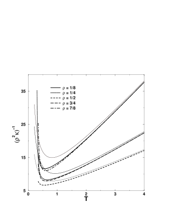
FIG. 3.: The inverse compressibility $(\rho^{2}\kappa)^{-1}$ as a function of temperature $T$. Shown are the [4,6]–PAs to the 10^th order series on the s. c. lattice. The thin lines through each pair depict the values of $(\rho^{2}\kappa)^{-1}$ from the HTSE for free spinless fermions on a s.c. lattice at the corresponding densities $\rho$.

Again we find a quasi–linear behavior below a certain temperature. By comparing with a HTSE for spinlesss fermions on the s. c. lattice we see that differences in the compressibility between the DE model and noninteracting spinless fermions are small and only become relevant at low temperatures. This means that the DE model at high temperatures behaves pretty much like a system of non–interacting spinless fermions at least with respect to charge excitations. We do not see any evidence for unusual behavior in $\kappa$ that would be indicative of some kind of charge ordering. However, this is not conclusive since one would expect unusual behavior to occur at a specific wavevector related to the filling, and hence it is not surprising to see nothing in our $q=0$ compressibility.

To connect more closely to the CMR effect it would be necessary to calculate the magnetoresistance (MR) $\rho_{c}(h)/\rho_{c}(h=0)-1$, where $\rho_{c}$ is the resistivity and $h$ the applied magnetic field. The MR arises from two sources. One is a change in the scattering time due to the magnetic field, which modifies the dynamical properties, the other is the dependence of the bandwidth on the magnetic field, which is a static effect. The latter is large in the DE model as the effective bandwidth is strongly dependent on the alignment of the local spins. In a fermi-gas, the compressibility is proportional to the effective mass. Thus, we can capture this bandwidth effect in the magneto–compressibility (MC) $\kappa(h)/\kappa(h=0)-1$. In Fig. 4, we show the MC for various densities as a function of inverse temperature. As expected, and desired, it is always negative. For intermediate $\rho$ we observe saturation of the MC around $\beta=1$ corresponding to the appearance of linear behavior of $\chi^{-1}$. This does not agree with the behavior observed in the MR of the real materials. Also the concentration dependence of the MC is inconsistent with that of the MR; the higher the concentration of $e_{g}$ electrons the larger is the MC. This can be understood by noting that for larger $\rho$ there is effectively more spin to be polarized by the magnetic field. One way to resolve this discrepancy would be to assume that the dynamic effects in the MR are more important than the static ones captured within the MC.

FIG. 4.: The MC as defined in the text as a function of $\beta$. Shown are two PAs (upper:[4,6] lower: [6,4]) for the respective densities $\rho$.

In this letter we have provided the first exact results for the ferromagnetic Kondo lattice model in terms of a HTSE. Although we have used a smaller spin value than is realized in the CMR materials, the $t_{2g}$ spin length is set to $1/2$ instead of $3/2$, this should not affect $T_{c}$ much as, to leading order for $J_{H}\to\infty$, the spin-length drops out of the problem. The analytic structure of the resulting series is governed by a singularity on the imaginary axis, which we indentify as being responsible for the crossover from the high–T range to the physically interesting temperature range below the bandwidth. This behavior is probably also typical of other itinerant systems, although the DE model in the $J_{H}\to\infty$ limit is unusual, because the local moment $\sum_{i}<(S_{i}^{z})^{2}>$ is a constant, and does not depend on temperature. Our estimates for the magnetic transition temperature are close to the experimentally observed ones. Mean–field theory, as mimicked by the Bethe lattice series, overestimates $T_{c}$ by about $25\%$. There are also some unusual features associated with the charge degrees of freedom as indicated by the slightly ferrimagnetic behavior, but our calculations are not sufficient to study long-range charge order. Nevertheless, the tendencies towards charge ordering should imply a large sensitivity of the CMR materials towards Jahn–Teller ordering effects. In further work we will investigate the wave-vector dependence of the compressibility to address this question. Our results for the magneto–compressibility indicate that dynamic effects are responsible for the CMR effect, and that a static description may be inadequate.

Acknowledgements

We thank A. R. Bishop, S. Trugman, G. Baker, Jr., and D. Wallace for many illuminating discussions. This work is supported in part by NSF grant number DMR-9616574.

Thanks a lot.

Best Regards, Rajiv and by the University of California campus laboratory collaboration (CLC).

REFERENCES

- [1] R. M. Kusters et al, Physica B 155, 362 (1989).
- [2] K. Chahara et al, Appl. Phys. Lett. 71, 1990 (1993).
- [3] R. von Helmholt, Phys. Rev. Lett. 71, 2331 (1993).
- [4] C. Zener, Phys. Rev. 82, 403 (1951).
- [5] P. W. Anderson and H. Hasegawa, Phys. Rev 100, 675 (1955).
- [6] P. G. deGennes, Phys. Rev. 118, 141 (1960).
- [7] K. Kubo and N. Ohata, J. Phys. Soc. Jpn. 33, 21 (1972).
- [8] N. Furukawa, J. Phys. Soc. Jpn, 33, 21 (1994).
- [9] A. J. Millis, P. B. Littlewood, and B. I.Shraiman, Phys. Rev. Lett. 74, 5144 (1995).
- [10] H. Röder, J. Zang, and A. R. Bishop, Phys. Rev. Lett. 76, 1356 (1996).
- [11] see e. g. J. M. Salamon et al, J. Appl. Phys. Lett. 68, 1576 (1996).
- [12] J. Zang, H. Röder, A. R. Bishop, and S. A. Trugman, preprint cond-mat/9606148.
- [13] E. Müller–Hartmann and E. Dagotto, preprint cond-mat/9605041.
- [14] J. Riera, K. Hallberg, and E. Dagotto, preprint cond-mat/9609111.
- [15] R. R. P. Singh and R. L. Glenister, Phys. Rev. B46, 11871 (1992).
- [16] G. A. Baker, Jr., H. E. Gilbert, J. Eve, and G. S. Rushbrooke, Phys. Rev. 164, 800 (1967).
- [17] G. A. Baker, Jr. and P. Graves–Morris, Padé Approximants, Cambridge University Press, Cambridge 1996
- [18] R. M. White, Quantum Theory of Magnetism, Springer Series in Solid–State Sciences 32, pp. 107, Springer Berlin 1983
- [19] C. M. Varma, preprint cond-mat/9608086.