Low temperature Correlation lengths of Bilayer Heisenberg Antiferromagnets and Neutron Scattering

Abstract

The low temperature correlation length and the static structure factor are computed for bilayer antiferromagnets such as YBa₂Cu₃O₆. It is shown that energy integrated two-axis scan in neutron scattering experiments can be meaningfully interpreted to extract correlation length in such bilayer antiferromagnets despite intensity modulation in the momentum perpendicular to the layers. Thus, precise measurements of the spin-spin correlation length can be performed in the future, and the theoretical predictions can be tested. It is also shown how the same correlation length can be measured in nuclear magnetic resonance experiments.

Nearly thirty five years ago Birgeneau, Skalyo and Shirane[1] invented a neutron scattering method, known as the energy integrated two-axis scan (ETAS), whereby the spin-spin correlation lengths of layered magnets can be measured without explicitly measuring the dynamic structure factor for all energy and momentum transfers and then integrating over the energy, known as the three axis scan. Except for special circumstances, three axis scan to measure correlation length is difficult.

The underlying principles of ETAS are an analog energy integration performed by using a special geometry and the reliance on the dominance of low energy scattering—the method is especially effective when the critical scattering dominates. In recent years, ETAS has served us well in unravelling the magnetic fluctuations of the parent compound of one of the high temperature superconductors, namely the La₂CuO₄[2]. The experimental results are in excellent agreement with our theoretical understanding of these two-dimensional magnets[3]. Unfortunately, the method does not appear to be readily extendable to a wide class of high temperature superconductors with close magnetic bilayers or triple layers within the unit cell; a particularly important example is ${\rm YBa_{2}Cu_{3}O_{6}}$, which has a close pair of magnetic planes within the unit cell, but it is otherwise a square lattice spin $S=1/2$ Heisenberg antiferromagnet. The reason for the difficulty of using ETAS is an intensity modulation[4] with the momentum transfer perpendicular to the planes.

It is the purpose of the present paper to (a) derive the low temperature properties of such bilayer antiferromagnets and (b) to show how ETAS can be extended to such bilayer antiferromagnets. It is hoped that future experiments using ETAS will be able to provide us with precise measurements of the antiferromagnetic correlation lengths in these materials, which should be of great help in understanding the magnetic flutuations of these bilayer superconductors. We also briefly remark how the same correlation length can be also measured by measuring the Cu relaxation rate in nuclear magnetic resonance (NMR) experiments.

The Heisenberg model for a spin-$S$, nearest neighbor, square lattice, bilayer antiferromagnet is

$$H=J_{\parallel}\sum_{\langle ij\rangle,p}{\bf S}_{i}^{(p)}\cdot{\bf S}_{j}^{(p)}+J_{\perp}\sum_{i}{\bf S}_{i}^{(1)}\cdot{\bf S}_{i}^{(2)}.$$ (1)

The sum in the first term is over the nearest neighbor pairs in each plane, where the plane index $p$ takes two values 1 and 2. The second term represents the coupling between the planes. The exchange constants $J_{\parallel}$ and $J_{\perp}$ are both positive.

The low energy, long wavelength properties of the two dimensional Heisenberg model is well described by the quantum $O(3)$ nonlinear $\sigma$-model[5]. Here, we shall consider its generalization to coupled bilayers. The Euclidean action for this system can be written down on general symmetry grounds[5], but it can also be derived from a $(1/S)$ expansion[6]. The action is

$$S = \int^{u}_{0}dx_{0}\int d^{2}x\Bigg{[}\sum_{p=1}^{2}\left({1\over 2g_{0}}|\partial_{\mu}\hat{{\bf\Omega}}^{(p)}|^{2}-h_{0}\sigma^{(i)}\right)$$ (2)

$$+ {1\over 2g_{\perp}^{0}}|\hat{{\bf\Omega}}^{(1)}-\hat{{\bf\Omega}}^{(2)}|^{2}-{1\over 2g_{t}^{0}}(\hat{{\bf\Omega}}^{(1)}\times\partial_{0}\hat{{\bf\Omega}}^{(1)})\cdot(\hat{{\bf\Omega}}^{(2)}\times\partial_{0}\hat{{\bf\Omega}}^{(2)})\Bigg{]},$$ (3)

where $\sigma^{(p)}$ is the component of the staggered field $\hat{{\bf\Omega}}^{(p)}$ in the direction of the staggered magnetic field $h$. Here, all the coupling constants and dimensional variables have been scaled to their dimensionless forms. The label $\mu=1,2$ denotes the spatial directions, and $\mu=0$ corresponds to the imaginary time direction. The extent in the imaginary time direction is given by $u$, where $c_{0}$ is the spin-wave velocity. For mathematical purposes, it is possible to extend the action to dimensions, $d$, other than 2 and to the general symmetry group $O(N)$. It is only for $d=2$ and $N=3$, however, that the model represents a bilayer antiferromagnet. Since there are no difficulties in working directly with $d=2$ and $N=3$, we shall use these parameters throughout the paper. For later convenience, we define $\tilde{h}_{0}=h_{0}g_{0}$, $\tilde{\gamma}_{\perp}^{0}={2g_{0}\over g_{\perp}^{0}}$, and $\tilde{\delta}_{t}^{0}={g_{0}\over 2g_{t}^{0}}$.

The relations between the $\sigma$-model parameters and the Heisenberg model parameters are known in the large-$S$ limit[6]. After correcting minor errors, the correct relations, in the limit $S\to\infty$, are $g_{0}={\hbar c_{0}\sqrt{1-\tilde{\delta}_{t}^{0}}\Lambda\over\rho_{s}^{0}}$, $g_{\perp}^{0}={\hbar c_{0}\sqrt{1-\tilde{\delta}_{t}^{0}}\Lambda(\Lambda a)^{2}\over\rho_{\perp}^{0}}$, $g_{t}^{0}={4\hbar c_{0}\Lambda\over\rho_{\perp}^{0}\sqrt{1-\tilde{\delta}_{t}^{0}}}$, and $u={\beta\hbar c_{0}\sqrt{1-\tilde{\delta}_{t}^{0}}\Lambda}$, where $\tilde{\delta}_{t}^{0}={J_{\perp}\over 8J_{\parallel}+J_{\perp}}$; the spin-stiffness constants are $\rho_{s}^{0}=J_{\parallel}S^{2}$ and $\rho_{\perp}^{0}=J_{\perp}S^{2}$, and the spin wave velocity is $c_{0}={aS\over\hbar}\sqrt{2J_{\parallel}(4J_{\parallel}+J_{\perp})}$. The quantity $a$ is the lattice constant of the Heisenberg model, and the momentum cutoff is given by $\Lambda={\sqrt{2\pi}\over a}$ to conserve the number of degrees of freedom.

Our calculations show explicitly [7] that the angular momentum coupling between the layers is irrelevant for weakly coupled bilayer systems such as ${\rm YBa_{2}Cu_{3}O_{6}}$, although it breaks the “Lorentz invariace” and renormalizes the spin-wave velocity. The angular momentum coupling term also reduces to a higher gradient term when the number of layers tends to infinity. We shall omit this term from our further discussion.

This bilayer model has a massless mode and a massive mode. We can see this by simply expanding the action to quadratic order:

$$S_{2} = \int^{u}_{0}dx_{0}\int d^{2}x{1\over 4g_{0}}\Bigg{[}|\partial_{\mu}({\mbox{\boldmath$\pi$}}^{(1)}+{\mbox{\boldmath$\pi$}}^{(2)})|^{2}+\tilde{h}_{0}|{\mbox{\boldmath$\pi$}}^{(1)}+{\mbox{\boldmath$\pi$}}^{(2)}|^{2}$$ (4)

$$+ |\partial_{\mu}({\mbox{\boldmath$\pi$}}^{(1)}-{\mbox{\boldmath$\pi$}}^{(2)})|^{2}+(\tilde{h}_{0}+\tilde{\gamma}_{\perp}^{0})|{\mbox{\boldmath$\pi$}}^{(1)}-{\mbox{\boldmath$\pi$}}^{(2)}|^{2}\Bigg{]},$$ (5)

where ${\mbox{\boldmath$\pi$}}^{(i)}$ is the transverse component of $\hat{\bf\Omega}^{(i)}$. In the absence of staggered field $\tilde{h}_{0}=0$, the symmetric combination is gapless, and the antisymmetric combination has a gap $\sqrt{\tilde{\gamma}_{\perp}^{0}}$, which will be called the bare dimensionless bilayer gap; the bare dimensional bilayer gap is given by $\hbar c_{0}\Lambda\sqrt{\tilde{\gamma}_{\perp}^{0}}$. At finite temperatures, the massless mode becomes massive due to interactions, which is a topic of this paper.

We carry out one-loop momentum-shell calculations similar to those of Ref. [5] and obtain the following renormalization group equations

$${dg\over dl} = -g+{g^{2}\over 8\pi}\left[{\coth({g\over 2t}\sqrt{1+\tilde{h}})\over\sqrt{1+\tilde{h}}}+{\coth({g\over 2t}\sqrt{1+\tilde{h}+\tilde{\gamma}_{\perp}})\over\sqrt{1+\tilde{h}+\tilde{\gamma}_{\perp}}}\right],$$ (6)

$${dt\over dl} = {gt\over 8\pi}\left[{\coth({g\over 2t}\sqrt{1+\tilde{h}})\over\sqrt{1+\tilde{h}}}+{\coth({g\over 2t}\sqrt{1+\tilde{h}+\tilde{\gamma}_{\perp}})\over\sqrt{1+\tilde{h}+\tilde{\gamma}_{\perp}}}\right],$$ (7)

$${d\tilde{h}\over dl} = 2\tilde{h},$$ (8)

$${d\tilde{\gamma}_{\perp}\over dl} = 2\tilde{\gamma}_{\perp}-{g\tilde{\gamma}_{\perp}\over 4\pi}{\coth({g\over 2t}\sqrt{1+\tilde{h}+\tilde{\gamma}_{\perp}})\over\sqrt{1+\tilde{h}+\tilde{\gamma}_{\perp}}},$$ (9)

where $e^{l}$ is the length rescaling factor. The variable $t$ is the dimensionless temperature variable. The dimensionless thickness of the slab in the imaginary time direction $u=g/t$ satisfies a simple scaling relation given by $(g/t)=(g_{0}/t_{0})e^{-l}$.

The zero temperature flows of the renormalization group equations are shown in Fig.1. There are two phases, separated by a separatrix between the two unstable fixed points $(g=4\pi,g_{\perp}=\infty)$ and $(g=8\pi,g_{\perp}=0)$; the former is the fixed point of the single layer case[5]. There are two stable fixed points. The ordered-phase fixed point is located at $(0,0)$, where both the in- and the inter-plane couplings are infinitely strong. The disordered-phase fixed point is located at $(\infty,\infty)$, where the system becomes totally disordered. Although quantum nonlinear $\sigma$-model is a very accurate description of the low energy physics in or near the ordered phase[5], far into the disordered phase, such a continuum theory can not be expected to be valid.

In the bilayer, $S=1/2$ Heisenberg model, a quantum phase transition takes place when $J_{\perp}\geq 2.55J_{\parallel}$[10]. In the $\sigma$-model, the phase transtion takes place at a critical value of $g$ for any $g_{\perp}$. At present, we do not have an accurate mapping between the Heisenberg model parameters and the $\sigma$-model parameters allowing us to relate the quantum disordered phases of these two models. In the quantum disordered phase, the large-$S$ analysis is not appropriate because it relies on the existence of goldstone modes that are not present in this phase.

The parameters applicable to ${\rm YBa_{2}Cu_{3}O_{6+x}}$ lie in the ordered phase, where $\tilde{\gamma}_{\perp}^{0}\sim{J_{\perp}\over J_{\parallel}}\ll 1$, and $g$ is below the critical value required for the phase transition to the quantum disordered phase at $T=0$. Therefore, the system is in the renormalized classical regime[5]. Also, from experiments, it is known that the ground state is an ordered Néel state and that $J_{\perp}\sim 0.1J_{\parallel}$[9].

To proceed further, we need an analytical solution of the renormalization group equations. We have obtained a good appoximation to the solution based on the following observations. In the renormalized classical regime, the bilayer gap $\sqrt{\tilde{\gamma}_{\perp}}$ is initially much smaller than unity, but increases as $\sqrt{\tilde{\gamma}_{\perp}}\propto e^{\alpha(l)l/2}$, where $\alpha(l)<2$, but tends to 2 for large $l$. We can therefore consider two regions, $\tilde{\gamma}_{\perp}\ll 1$ in region (I), and ${d\tilde{\gamma}_{\perp}\over dl}\simeq 2\tilde{\gamma}_{\perp}$ in the region (II). We solve the renormalization group equations separately in regions (I) and (II), and then join the two solutions together to get the final answer. In (I), we replace $\sqrt{1+\tilde{\gamma}_{\perp}}$ by unity and obtain

$${1\over t_{0}}-{1\over t_{1}}={1\over 2\pi}\left[\ln\sinh({g_{0}\over 2t_{0}})-\ln\sinh({g_{0}\over 2t_{0}}e^{-l_{1}})\right],$$ (10)

$$\tilde{\gamma}_{\perp}^{1}={t_{0}\over t_{1}}\tilde{\gamma}_{\perp}^{0}e^{2l_{1}},$$ (11)

where $(l_{1},t_{1},\tilde{\gamma}_{\perp}^{1})$ are the variables at the endpoint of (I). In (II), we use ${d\tilde{\gamma}_{\perp}\over dl}=2\tilde{\gamma}_{\perp}$ and get

$${1\over t_{1}}-{1\over t}={1\over 4\pi}\ln\left[{\sinh({g_{0}\over 2t_{0}}e^{-l_{1}})\sinh({g_{0}\over 2t_{0}}e^{-l_{1}}\sqrt{1+\tilde{\gamma}_{\perp}^{1}})\over\sinh({g_{0}\over 2t_{0}}e^{-l})\sinh({g_{0}\over 2t_{0}}e^{-l_{1}}\sqrt{e^{-2(l-l_{1})}+\tilde{\gamma}_{\perp}^{1}})}\right].$$ (12)

The initial condition $\tilde{\gamma}_{\perp}^{0}\ll 1$ guarantees that the crossover between (I) and (II) is smooth, namely, $\tilde{\gamma}_{\perp}^{1}\ll 1$ and ${d\tilde{\gamma}_{\perp}\over dl}|_{l_{1}}\simeq 2\tilde{\gamma}_{\perp}^{1}$. Since we can choose $l_{1}$ such that $\tilde{\gamma}_{\perp}^{0}\ll e^{-2l_{1}}\ll 1$, this garuantees that $\tilde{\gamma}_{\perp}^{1}\ll 1$ from Eq. (11). The initial temperature is low enough that both ${g_{0}\over 2t_{0}}$ and ${g_{0}\over 2t_{0}}e^{-l_{1}}$ are much larger than unity. Following Eq. (10), we get ${1\over t_{1}}\simeq{1\over t_{0}}(1-{g_{0}\over 4\pi})$. At this point, the second term in Eq. (9) becomes negligible because ${g\over 4\pi}{\coth({g\over 2t}\sqrt{1+\tilde{\gamma}_{\perp}})\over\sqrt{1+\tilde{\gamma}_{\perp}}}\simeq{g_{0}t_{1}\over 4\pi t_{0}}e^{-l_{1}}={g_{0}\over 4\pi-g_{0}}e^{-l_{1}}\ll 2$; therefore ${d\tilde{\gamma}_{\perp}\over dl}|_{l_{1}}\simeq 2\tilde{\gamma}_{\perp}^{1}$ is also true.

The two solutions can now be combined together to get

$${1\over t_{0}}-{1\over t}={1\over 4\pi}\ln\left[{\sinh^{2}({g_{0}\over 2t_{0}})\over\sinh({g_{0}\over 2t_{0}}e^{-l})\sinh\left({g_{0}\over 2t_{0}}\sqrt{e^{-2l}+e^{-2l_{1}}\tilde{\gamma}_{\perp}^{1}}\right)}\right].$$ (13)

The single layer result

$${1\over t_{0}}-{1\over t}={1\over 2\pi}\left[\ln\sinh({g_{0}\over 2t_{0}})-\ln\sinh({g_{0}e^{-l}\over 2t_{0}})\right]$$ (14)

is trivially recovered when the bilayer gap is much smaller than the inverse correlation length, that is, $\sqrt{\tilde{\gamma}_{\perp}^{0}}\ll e^{-l}$.

In the limit of large $l$, the solution has the asymptotic form of ${2\over t}={2\over t_{\rm eff}}-{l\over 2\pi}$, where

$${1\over t_{\rm eff}}={1\over t_{0}}(1-{g_{0}\over 4\pi})+{1\over 4\pi}\ln\left[{2g_{0}\over t_{0}}\sinh({g_{0}\over 2t_{0}}\sqrt{\tilde{\gamma}_{\perp}^{0}(1-{g_{0}\over 4\pi})})\right].$$ (15)

This is identical to the low temperature limit of the solution of a classical single-layer $\sigma$-model: ${1\over t^{\rm cl}}={1\over t^{\rm cl}_{0}}-{l\over 2\pi}$. Thus, we can map the quantum bilayer model to the classical single layer model by identifying ${2\over t_{\rm eff}}={1\over t^{\rm cl}_{0}}$ and ${2\over t}={1\over t^{\rm cl}}$. The remaining arguments as to how to combine the classical two-loop result, along with the conversion of the prefactor from the continuum to the lattice, are the same as those given in Ref. [5]. We get

$$\xi={e\over 8}\Lambda^{-1}{t_{\rm eff}\over 4\pi}e^{4\pi\over t_{\rm eff}},$$ (16)

with the exact prefactor determined in Ref. [8].

An important result is that the argument of the exponential is twice of that of the single layer case. This factor of $2$ comes from the mapping between the bilayer model and the single layer model. To get a feeling for this factor, it is instructive to consider a classical bilayer model given by the action $S={1\over t^{\rm cl}}\int d^{2}x\left[\sum_{i=1}^{2}\left(|\partial_{\mu}\hat{{\bf\Omega}}^{(i)}|^{2}-\tilde{h}\sigma^{(i)}\right)+{\tilde{\gamma}_{\perp}\over 2}\left|\hat{{\bf\Omega}}^{(1)}-\hat{{\bf\Omega}}^{(2)}\right|^{2}\right]$. To map it on to the single layer model, we need to define a new field $\hat{{\bf\Omega}}$, where the transverse components are given by ${\mbox{\boldmath$\pi$}}={1\over 2}({\mbox{\boldmath$\pi$}}^{(1)}+{\mbox{\boldmath$\pi$}}^{(2)})$, and the longitudinal component is given by $\sigma=\sqrt{1-|{\mbox{\boldmath$\pi$}}|^{2}}$. This can be accomplished by integrating out the massive fields ${1\over 2}({\mbox{\boldmath$\pi$}}^{(1)}-{\mbox{\boldmath$\pi$}}^{(2)})$. The result is the new action $S^{\prime}={2\over t^{\rm cl}}\int d^{2}x\left(|\partial_{\mu}\hat{{\bf\Omega}}|^{2}-h\sigma\right)$, consistent with our previous result.

When temperature is low enough such that ${g_{0}\over 2t_{0}}\sqrt{\tilde{\gamma}_{\perp}^{0}}>1$, the correlation length can be written as

$$\xi={e\over 8}{\hbar c\over 4\pi\rho_{s}(0)}e^{4\pi\rho_{s}(0)\over k_{B}T},$$ (17)

where $\rho_{s}(0)$ is the renormalized spin stiffness constant, which within one-loop approximation is given by $\rho_{s}(0)=\rho_{s}^{0}\left[1-{g_{0}\over 4\pi}\left(1-{1\over 2}\sqrt{\tilde{\gamma}_{\perp}^{0}(1-{g_{0}\over 4\pi})}\right)\right]$. As discussed in Ref. [5], the formula can be used with $\rho_{s}(0)$ the exact spin stiffness constant of the bilayer Heisenberg model.

The numerical value of the spin stiffness constant can be obtained from spin-wave theory, and it is given by $\rho_{s}(0)=J_{\parallel}S^{2}Z^{2}_{c}(S)Z_{\chi}(S).$ For $S=(1/2)$, $J_{\perp}=0.08J_{\parallel}$[9], and up to order of $(1/S)$, we get $Z_{c}(S)=1.153,Z_{\chi}(S)=0.531,$ and $\rho_{s}(0)=0.176J_{\parallel}$. Therefore the correlation length is given by

$$\xi\simeq 0.25ae^{4\pi\rho_{s}(0)\over k_{B}T},$$ (18)

where $a$ is the lattice spacing. The exponential temperature dependence is identical to the single layer case, but the factor of 2 in the exponent should be noted.

The static structure factor can be obtained in the same way as in Ref. [5]. For the bilayer case, it contains two pieces, one for the symmetric combination of the unit vectors from each layer and the other for the antisymmetric combination. The notation in the $\sigma$-model is exactly the opposite to the notation in the Heisenberg model, since the unit vector field $\hat{{\bf\Omega}}^{(p)}$ in the $\sigma$-model is the continuum limit of the direction vector of the staggered spin operator $(-1)^{i+p}{\bf S}_{i}^{(p)}$ in the Heisenberg model. Our renormalization group equations show that in the long wavelength limit both pieces satisfy the following equation as in the single layer case[5]

$$S(k,t_{0})=e^{2l}\left({t_{0}\over t}\right)^{2}S(e^{l}k,t),$$ (19)

where $t\equiv t(l)$ is the running coupling constant and $k$ is defined with respect to the antiferromagnetic wavevector $(\pi/a,\pi/a)$.

For the symmetric piece, we evaluate the right hand side at $l=l^{*}$ such that we are far into the disordered regime, either because the correlation length is of order unity or because the rescaled wave vector $ke^{l}$ is sufficiently large. These requirements are satisfied by choosing a $l^{*}$ such that $\xi^{-2}(t_{0})e^{2l^{*}}+k^{2}e^{2l^{*}}=1$. When this condition is satisfied, we can approximate $S_{\rm s}[e^{l^{*}}k,t(l^{*})]$ by the Ornstein-Zernicke form

$$S_{\rm s}[e^{l^{*}}k,t(l^{*})]\simeq{t(l^{*})\over\xi^{-2}(l^{*})+k^{2}(l^{*})}.$$ (20)

Then,

$$S_{\rm s}(k,t_{0})={t_{0}^{2}\xi^{2}\over 2\pi}f(x),$$ (21)

where $x=k\xi$ and $f(x)={1+{1\over 2}\ln(1+x^{2})\over 1+x^{2}}$.

The antisymmetric piece can be obtained in a similar manner. When $l\simeq l^{*}$, the bilayer gap $\sqrt{\tilde{\gamma}_{\perp}}$ is increased by a factor $e^{l^{*}}$. At this point, it is safe to assume the Ornstein-Zernicke form

$$S_{\rm a}(e^{l^{*}}k,t(l^{*}))\simeq{2t(l^{*})\over e^{2l^{*}}(\xi^{-2}_{\perp}+k^{2})},$$ (22)

where $\xi_{\perp}$ is the length scale associated with the bilayer gap. Approximately, we have $\xi_{\perp}\simeq e^{-l^{*}}\sqrt{\tilde{\gamma}_{\perp}}/\Lambda\simeq\sqrt{(1-{g_{0}\over 4\pi})\tilde{\gamma}_{\perp}^{0}}/\Lambda$. In terms of the initial coupling constants, we get

$$S_{\rm a}(k,t_{0})\simeq{(2-{g_{0}\over 2\pi})t_{0}\over k^{2}+\xi_{\perp}^{-2}}.$$ (23)

The symmetric piece is dominant in the long-wavelength limit because

$${S_{\rm s}(0,t_{0})\over S_{\rm a}(0,t_{0})}\sim t_{0}{\xi^{2}\over\xi^{2}_{\perp}}\gg 1.$$ (24)

In ETAS, the wavevector of the incoming neutron ${\bf q}_{i}$ is fixed, while the outgoing neutrons in a direction perpendicular to the layers are collected, regardless of their energies. The transferred wavevector is given by ${\bf q}={\bf q}_{f}-{\bf q}_{i}$. Its in-plane component ${\bf q}_{\parallel}$ is a constant, ${\bf q}_{\parallel}=-{\bf q}_{i\parallel}$, while its perpendicular component is a variable, $q_{\perp}=q_{f}-q_{i\perp}$. For ${\bf q}_{\parallel}$ near reciprocal lattice vectors, the form factor is approximately a constant, and the intensity $I({\bf q}_{\parallel})$ is proportional to $\int_{0}^{\infty}dq_{f}S^{3\rm D}({\bf q},{\hbar^{2}\over 2m}(q_{f}^{2}-q_{i}^{2}))$, where $S^{3\rm D}({\bf q},\omega)$ is the 3D dynamic structure factor. It is related to the 2D dynamic structure factors by $S^{3\rm D}({\bf q},\omega)=\sin^{2}({q_{\perp}h\over 2})S_{\rm a}^{2\rm D}({\bf q}_{\parallel},\omega)+\cos^{2}({q_{\perp}h\over 2})S_{\rm s}^{2\rm D}({\bf q}_{\parallel},\omega)$, where $h$ is the distance between the two layers. The quantity $S_{\rm a}^{2\rm D}({\bf q}_{\parallel},\omega)$ corresponds to the antisymmetric spin combination with respect to the layers, symmetric in the $\sigma$-model sense, and $S_{\rm s}^{2\rm D}({\bf q}_{\parallel},\omega)$ to the corresponding symmetric spin combination, antisymmetric in the $\sigma$-model sense. In experiments one probes the region ${\bf q}_{\parallel}\approx{\bf G}$, where $\bf G$ is the nearest antiferromagnetic reciprocal lattice vector. Defining ${\bf k}={\bf q}_{\parallel}-{\bf G}$, we can rewrite the intensity in terms of the $\sigma$-mode

l structure factors, recalling that the definitions of the symmetric and the antisymmetric combinations get switched in going from the spin picture to the $\sigma$-model picture. The intensity contains two pieces, $I({\bf k})=I_{\rm s}({\bf k})+I_{\rm a}({\bf k})$, where

$$I_{\rm s}({\bf k}) \sim \int_{0}^{\infty}dq_{f}\sin^{2}{(q_{f}-q_{i\perp})h\over 2}S_{\rm s}^{2\rm D{\sigma}}({\bf k},{\hbar^{2}\over 2m}(q_{f}^{2}-q_{i}^{2})),$$ (25)

$$I_{\rm a}({\bf k}) \sim \int_{0}^{\infty}dq_{f}\cos^{2}{(q_{f}-q_{i\perp})h\over 2}S_{\rm a}^{2\rm D{\sigma}}({\bf k},{\hbar^{2}\over 2m}(q_{f}^{2}-q_{i}^{2})).$$ (26)

The $q_{\perp}$-modulation is unimportant in the critical region. The reason is that $S_{\rm s}^{2\rm D{\sigma}}({\bf k},\omega)$ is dominated by the critical fluctuations near $\omega=0$, where both $\sin^{2}\left({(q_{f}-q_{i\perp})h\over 2}\right)$ and ${d\omega\over dq_{f}}={\hbar^{2}\over m}q_{f}$ are essentially constants. Therefore, we can pull these factors out of the integal and obtain the intensity approximately proportional to the static structure factor, $I_{\rm s}({\bf k})\sim{m\over\hbar^{2}q_{i}}\sin^{2}\left({(q_{i}-q_{i\perp})\over 2}h\right)\int_{-E_{i}}^{\infty}d\omega S_{\rm s}^{2\rm D{\sigma}}({\bf k},\omega)\sim S_{\rm s}({\bf k},t_{0})$, where we have reverted to the previous notation by dropping the superscripts. The quantity $E_{i}$ is the incident neutron energy. For the antisymetric piece, we get an upper bound by neglecting the factor $\cos^{2}({q_{\perp}h\over 2}$), which is $\int_{0}^{\infty}dq_{f}S_{\rm a}^{2\rm D{\sigma}}({\bf k},{\hbar^{2}\over 2m}(q_{f}^{2}-q_{i}^{2}))\sim{m\over\hbar^{2}\langle q_{f}\rangle}S_{\rm a}({\bf k},t_{0})$, where $\langle q_{f}\rangle$ is some average of the wavevector. Because $S_{\rm s}(0,t_{0})\gg S_{\rm a}(0,t_{0})$, the intensity is dominated by the contribution from the symmetric piece. Therefore ETAS for a bilayer should yield information about the symmetric piece, hence the correlation length. The contribution of the antisymmetric piece should result in a small broad background.

The NMR relaxation rate for the in-plane Cu site will be given by[11] ${1\over T_{1}}\propto T^{3\over 2}\xi$, because the symmetric structure factor will dominate when the correlation length $\xi$ is large. Thus, the formula for the correlation length, Eq. (17), can also be tested in NMR experiments, as for the single layer La₂CuO₄[12].

In conclusion, we have computed the low temperature properties of bilayer antiferromagnets using a quantum nonlinear $\sigma$-model approach. Explicit results were given for the static structure factor and the correlation length. The correlation length diverges exponentially as $T\to 0$, but the striking feature is that the argument of the exponential function is a factor of 2 larger than the corresponding single layer case. We have also shown that ETAS and NMR can be used to test our theoretical predictions concerning the correlation length.

We thank O. Syljuåsen for discussions. This work was supported by the National Science Foundation, Grant. No. DMR-9531575.

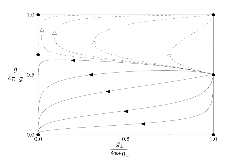
FIG. 1.: Zero temperature flow diagram.

REFERENCES

• [1] R. J. Birgeneau, J. Skalyo and G. Shirane, Phys. Rev. B 3, 1736 (1971)
• [2] Y. Endoh et al., Phys. Rev. B 37, 7443 (1988); K. Yamada et al., Phys. Rev. B 40, 4557 (1989).
• [3] For a theoretical review, see S. Chakravarty in High temperature superconductivity, edited by K. S. Bedell et al. (Addison-Wesley, Redwood City, 1990).For an experimental review, see M. Greven et al., Z. Phys. B 96, 465 (1995).
• [4] S. Shamoto et al. , Phys. Rev. B 48, 13817 (1993)
• [5] S. Chakravarty, B. I. Halperin, and D. R. Nelson, Phys. Rev. B 39, 2344 (1989).
• [6] A. V. Dotsenko, Phys. Rev. B 52, 9170 (1995)
• [7] The renormalization group equation for the angular momentum coupling is given by $d\tilde{\delta}_{t}/dl=-(\tilde{\delta}_{t}g/4\pi)\left[\coth\left({g\over 2t}\sqrt{{1+\tilde{h}+\tilde{\gamma}_{\perp}\over 1+\tilde{\delta}_{t}}}\right)/\sqrt{(1+\tilde{h}+\tilde{\gamma}_{\perp})(1+\tilde{\delta}_{t})}\right].$ Since $\tilde{\delta}_{t}$ always decreases and its initial value is very small, $\tilde{\delta}_{t}^{0}\propto{J_{\perp}\over J_{\parallel}}\ll 1$, it is irrelevant.
• [8] P. Hasenfratz and F. Niedermayer, Phys. Lett. B 268, 231 (1991)
• [9] D. Reznik et al., Phys. Rev. B 54, 14741 (1996); S. M. Hayden et al., Phys. Rev. B 54, 6905 (1996)
• [10] T. Matsuda and K. Hida, J. Phys. Soc. Jpn. 59, 2223 (1990); K. Hida, ibid 59, 2223 (1990); ibid 61, 1013 (1992); A. W. Sandvik and D. J. Scalapino, Phys. Rev. Lett. 72, 2777 (1994); A. V. Chubukov and D. K. Morr, Phys. Rev. B 52, 3521 (1995).
• [11] S. Chakravarty and R. Orbach, Phys. Rev. Lett. 64, 224 (1990).
• [12] T. Imai et al., Phys. Rev. Lett. 70, 1002 (1993).
Refer to caption