Monte Carlo simulation of a two-field effective Hamiltonian of complete wetting

Abstract

Recent work on the complete wetting transition for three dimensional systems with short-ranged forces has emphasized the role played by the coupling of order-parameter fluctuations near the wall and depinning interface. It has been proposed that an effective two-field Hamiltonian, which predicts a renormalisation of the wetting parameter, could explain the controversy between RG analysis of the capillary-wave model and Monte Carlo simulations on the Ising model. In this letter results of extensive Monte Carlo simulations of the two-field model are presented. The results are in agreement with prediction of a renormalized wetting parameter $\omega$.

There are a number of long standing controversies in the study of phase equilibria at fluid interfaces, related to wetting transitions for systems with short-ranged forces at the marginal dimension $d=3$ (for a recent review see for example [1]). The standard model used to describe fluctuation effects at wetting transitions is the effective interfacial Hamiltonian (also called the capillary wave (CW) model)

$$H[\ell({\bf y})]=\int d{\bf y}\Bigl{[}\frac{\Sigma_{\alpha\beta}(T)}{2}(\nabla\ell)^{2}+W(\ell)\Bigr{]}$$ (1)

where $\ell({\bf y})>0$ is a collective coordinate which represents the distance of the fluctuating fluid interface (separating bulk phases $\alpha$ and $\beta$, say) from a wall situated in the $\ell=0$ plane. Here $\Sigma_{\alpha\beta}$ is the interfacial stiffness coefficient and $W(\ell)$ is the effective binding potential which is usually specified as

$$W(\ell)=Ae^{-\kappa\ell}+Be^{-2\kappa\ell}+\bar{h}\ell$$ (2)

where $\kappa\equiv 1/\xi_{b}$ is the inverse bulk correlation length and $\bar{h}$ is proportional to a bulk ordering field. At a critical or complete wetting transition the mean interface displacement $\langle\ell\rangle$ (and other lengthscales) diverges as the external field approach critical values. For critical wetting, B is positive and the transition occurs at $\bar{h}=A=0$, corresponding to $T\rightarrow T_{W}$, the wetting temperature, while for complete wetting $A>0$, i.e. $T>T_{W}$ and the transition occurs for $\bar{h}\rightarrow 0$ for $T_{C}>T>T_{W}$.
One well known controversy concerns the critical wetting transition. For this case, RG calculations based on (1) (see for example [2]), predict strong non-universality for the critical exponents and amplitudes depending on the value of the wetting parameter $\omega(T)=k_{B}T\kappa^{2}/4\pi\Sigma_{\alpha\beta}$ at the transition temperature $T_{W}$. However, extensive Monte Carlo simulations of wetting in a three dimensional Ising model with nearest-neighbour interactions by Binder, Landau and Kroll [3], show only small deviations from mean-field theory consistent with $\omega\approx 0$. This contrasts sharply with the expected value $\omega\approx 0.8$ (at the temperature where the simulations were performed). Prompted by the discrepancy Gompper and Kroll [GK] [5] performed very accurate Monte Carlo simulations on a lattice version of (1) and found very good agreement with the renormalisation group treatment, leaving the controversy open.
More recently attention has focused on the complete wetting transition. For this case CW theory predicts that, while the critical exponents retain their mean-field values in the limit of $\bar{h}\rightarrow 0$, critical amplitudes are renormalised. For example, the mean distance $\langle\ell\rangle$ diverges at leading order as

$$\kappa\langle\ell\rangle\approx\theta\ln(1/\bar{h})$$ (3)

where $\theta$ depends on $\omega$. In particular for $\omega<2$, CW theory predicts $\theta^{CW}=1+\frac{\omega}{2}$. A new controversy appeared with the Ising model simulations of Binder, Landau and Ferrenberg [4], (at $\omega\sim 0.8$) consistent with $\theta\sim 1.6-1.8$, while the CW model predicts only $\theta^{CW}\approx 1.4$.

These results serve to emphasize that wetting at the marginal dimension is a rather special case and that the coarse-grained Hamiltonian (1) may not capture all the essential physics. Note that no such problems arise in two dimensions where the CW model yields predictions for universal critical exponents, amplitudes and scaling functions which are in excellent agreement with the exact Ising model results [6]. Motivated by this, several authors have undertaken a careful examination of the foundations of the RG theory and of the validity of the interfacial Hamiltonian. In particular Fisher and Jin [FJ] [7] initiated a method of systematically deriving interfacial Hamiltonian from an underlying Landau-Ginzburg-Wilson [LGW] model. For critical wetting, they suggested that (1) should be modified by allowing a position dependent stiffness coefficient and as a result argue that the transition may in fact be very weakly first-order. More recently, Parry and Boulter [PB] [8] argued that this is still not a sufficient modification of the CW model, since it does not account for fluctuations of the order parameter near the wall and depinning interface. Following the methods by [FJ][7], they introduced a two-field Hamiltonian for complete wetting

$$H[\ell_{1},\ell_{2}]=\int d{\bf y}\{\frac{1}{2}\Sigma_{\mu\nu}(\ell_{1},\ell_{2})\nabla\ell_{\mu}\cdot\nabla\ell_{\nu}+U(\ell_{1})+W(\ell_{2}-\ell_{1})\}$$ (4)

which is a functional of two collective coordinates $\ell_{1}({\bf y})$ and $\ell_{2}({\bf y})$ (representing the locations of generalised surfaces at the wall and the $\alpha\beta$ interface respectively) and ${\bf\Sigma}$ is a position dependent stiffness matrix [8]. The potential $U(\ell_{1})$ binds the lower surface to the wall and since the fluctuations of $\ell_{1}$ are small can be approximated by $U(\ell_{1})=\frac{1}{2}v_{0}\ell_{1}^{2}$. Here $v_{0}=\Sigma_{11}/\xi_{w\beta}^{2}$, where $\xi_{w\beta}$ is the the finite correlation length associated with the intrinsic fluctuations of the order parameter near the wall. The fluctuations of $\ell_{1}({\bf y})$ are not included in the CW and FJ models. The term $W(\ell_{2}-\ell_{1})$ is similar to the binding potential in (2). In the limit of complete wetting, $\ell_{2}$ unbinds from the wall while $\ell_{1}$ remains bound. In their RG analysis, [PB] show show that the coupling to a weakly fluctuating field results in an effective value of the wetting parameter. In the limit $v_{0}\rightarrow\infty$ or $\xi_{w\beta}\rightarrow 0$ the fluctuations of the lower surface are completely suppressed and the CW/FJ result $\theta^{CW}=1+\frac{\omega}{2}$ is recovered. In the other limit, $v_{0}\rightarrow 0$ or $\xi_{w\beta}\rightarrow\infty$, the Hamiltonian (4) can be written in terms of center of mass coordinates which gives an effective stiffness coefficient $\Sigma^{-1}=\Sigma_{22}^{-1}+\Sigma_{11}^{-1}$ and results in a capillary parameter $\omega_{eff}=\omega_{2}+\omega_{1}$. For intermediate values of $v_{0}$, linear [9] and non-linear RG analysis [10] predict that the effective capillary parameter is

$$\omega_{eff}=\frac{k_{B}T\kappa^{2}}{4\pi\Sigma_{22}}+\frac{k_{B}T\kappa^{2}}{4\pi(\Sigma_{11}+v_{0}/\Lambda^{2})}$$ (5)

Consequently, the critical amplitude $\theta$ is given by $\theta=\theta^{CW}+\Delta\theta$ with

$$\Delta\theta=\frac{1}{2}\Bigl{(}\frac{k_{B}T\kappa^{2}}{4\pi(\Sigma_{11}+v_{0}/\Lambda^{2})}\Bigr{)}.$$ (6)

where $\Lambda$ is a momentum cutoff. They estimated [9] $\Delta\theta\approx 0.3\pm 0.1$, which gives the prediction $\theta\sim 1.7\pm 0.1$, in reasonable agreement with the Ising simulations in the complete wetting regime. For the subsequent development in theory, it seems important that [PB] theory is tested by independent methods. The crucial prediction is that the capillary parameter is renormalised due to the coupling to a field $\ell_{1}({\bf y})$ which only weakly fluctuates. To this end, in this letter, the Monte Carlo studies of critical wetting by [GK] [5] have been generalised to the two-field Hamiltonian in the complete wetting regime.

The simulations were performed on a lattice version of (4). The two surfaces $\ell_{1}$ and $\ell_{2}$ are modelled by two parallel $L\times L$ square lattices with periodic boundary conditions. The variables $x(i,j)$ and $y(i,j)$ are the distances of the site $(i,j)$ of the lower ($\ell_{1}$) and upper ($\ell_{2}$) surface respectively, from the wall (located at zero). The uncoupled gradient terms are approximated by

$$\frac{1}{16\pi\omega_{1}}\sum_{(i,j),\delta}(x(i,j)-x_{\delta}(i,j))^{2},\ \ \ \ \ \ \frac{1}{16\pi\omega_{2}}\sum_{(i,j),\delta}(y(i,j)-y_{\delta}(i,j))^{2}$$ (7)

where $\delta$ indicate the four nearest-neighbours of the site $(i,j)$ and the sum is over all sites $(i,j)$ for $i,j=1,...,L$, and $x$ and $y$ are measured in units of the bulk correlation length $\xi_{b}$. To test the program, the potential (2) is first chosen as $A=0,B=1$ (critical wetting), $\Sigma_{11}$ is set very large to suppress the fluctuations of the lower surface $\ell_{1}$, the cross-gradient coupling term $\Sigma_{12}$ is kept to zero and $\omega_{2}$ takes the values given by [GK] [5]. The results are in very good agreement with their founding. For complete wetting, the potential is chosen as $A=1$ and $B=0$ and the cross-gradient coupling term $\Sigma_{12}$ kept to zero [9]. The lattice size $L$ is varied between $10$ and $40$ to study finite-size effects. The SOS approximation is adopted and $x(i,j)$ and $y(i,j)$ are treated as continuous variables to avoid problems related to roughening. For simplicity we ignore the exponentially small position-dependence of the stiffness matrix elements since they play no role in determining the increment $\Delta\theta$ [9]. The hard wall condition ($y\geq x$) is used here, although the prediction (5) is also valid in a soft wall approximation [9, 10] (see for example [5] for a discussion regarding the CW model). The wetting parameters are chosen as $\omega_{1}=1$ and $\omega_{2}=0.8$, and so the maximum increment to $\theta$ is $\Delta\theta^{max}=0.5$ (corresponding to $v_{0}=0$).
A Metropolis algorithm has been used on a Dec Alpha 3600. At each Monte Carlo sweep, one of the two surfaces is chosen at random $2L^{2}$ times, and then a randomly picked site $(i,j)$ is updated by a random number in the interval $[-z_{m},+z_{m}]$; $z_{m}$ is set so that approximately 50% of the updates are accepted (but other values have also been used to test the convergence rate). The first $10^{4}$ sweeps are discarded to thermalise the system and $10^{6}$ sweeps are used to calculate the averages. The block average method is used to obtain statistical errors and the integrated autocorrelation time $\tau_{int}$ is calculated as in Madras and Sokal [11]. For example for the parameter $v_{0}=100$ and field $h=0.1$, $\tau_{int}=15$ and for $h=0.01$, $\tau_{int}=113$, while for $v_{0}=0.05$ and field $h=0.1$, $\tau_{int}=25$ and for $h=0.01$, $\tau_{int}=159$. For a given value of the parameter $v_{0}$ the average distance $\langle y\rangle$ of the upper surface from the wall, is calculated for several values of the fields $h$. Firstly, to approximate the limiting value $v_{0}\approx\infty$ or $\xi_{w\beta}\approx 0$, $v_{0}$ is set at $v_{0}=100$. In Figure $1$, $\langle y\rangle$ is plotted against $\ln(1/h)$ as in eq.(3). The values of $\langle y\rangle$ lie on a straight-line and a logarithmic regression gives a slope $\theta=1.43\pm 0.008$. The other limit, $v_{0}\approx 0$ or $\xi_{w\beta}\approx\infty$, is approximated by $v_{0}=0.05$. For smaller values of $v_{0}$ the fluctuations become very large, the autocorrelations increase and the simulations are not reliable. The values of $\langle y\rangle$, plotted against $\ln(1/h)$ in Figure $1$, show that they lie on a straight-line, but now with a slope $\theta=1.65\pm 0.02$. Figure $1$ suggest that $\theta$ is $v_{0}$ dependent and other intermediate values of $v_{0}$ are chosen to show this. In Figure $2$ are plotted the fitted values of the slopes $\theta$ corresponding to different values of $v_{0}$ for lattice sizes $L=20,40$. Importantly, the graph shows that the value of $\theta$ is indeed larger than the CW prediction $\theta^{CW}\approx 1.4$ for finite values of $v_{0}$, consistent with (6). Due to the dependence on the cutoff $\Lambda$ a precise quantitative comparison between simulation and theory is not possible. Nevertheless a fit of the numerical results to the theoretical prediction (6) yields a value for the cutoff $\Lambda$ close to unity, which is encouraging. We also note that as $v_{0}$ increases, the increment $\Delta\theta$ decreases and we recover the CW model prediction $\theta^{CW}\approx 1.4$ as $v_{0}\rightarrow\infty$. For small $v_{0}$ the measured value of $\theta$ is considerably bigger than the CW result and increases non-linearly with $1/v_{0}$. As mentioned above, the limiting value should be $\theta=1.9$, but this can not be reached in the simulations since it corresponds to infinite fluctuations. Unfortunately, extrapolation to $v_{0}=0$ is not possible either, given the non-linear dependence of $\theta$ on $v_{0}$ and large finite-size effects which would occur in this limit. Nevertheless the observed increase of $\theta$ with $v_{0}$ testifies to the strong influence of the coupling between the two fields and is certainly consistent with the basic prediction of the coupled Hamiltonian theory.
In the light of [PB] theory [8], the results are interpreted as follow: for very large values of $v_{0}$ the lower surface is very stiff and it does not fluctuate, hence the capillary wave result of $\theta^{CW}\approx 1.4$ is recovered. For decreasing values of $v_{0}$, even small fluctuations in the lower surface coupled to the upper surface produce a change in the critical amplitude $\theta$ as predicted by the theory and also in agreement with the Ising model simulations. This is the first time that RG predictions of an effective Hamiltonian, simulations on the Ising model and simulations of the same effective Hamiltonian are in qualitatively and quantitatively agreement. It would be interesting to extend this work to critical wetting and investigate if (4) can shed light on the controversy there. However this is beyond the scope of the present letter.

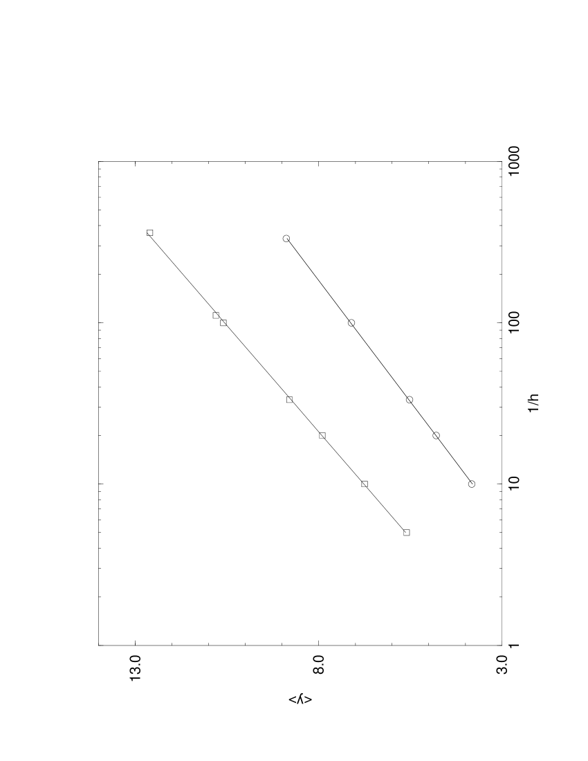
Figure 1: Mean interface displacement $\langle y\rangle$ against $\log(1/h)$, for $v_{0}=100$ (circles) and $v_{0}=0.05$ (squares). The error bars are within the symbols. The solid lines are the logarithmic regressions.

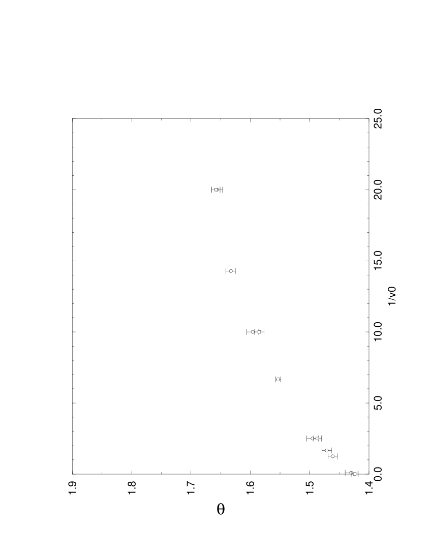
Figure 2: Critical amplitude $\theta$ as a function of the inverse parameter $v_{0}$, for lattice size $L=20$ (circles) and $L=40$ (squares).

References

- [1] A.O. Parry, J. Phys.: Cond. Matter 8, 10761 (1996).
- [2] E. Brézin, B.I. Halperin and S. Liebler, Phys. Rev. Lett. 50, 1387 (1983).
- [3] K. Binder, D.P. Landau and D.M. Kroll, Phys. Rev. Lett. 56, 2272 (1986).
- [4] K. Binder, D.P. Landau and A.M Ferrenberg, Phys. Rev. Lett. 74, 298 (1995).
- [5] G. Gompper and D.M. Kroll, Europhysics Letters 5, 49 (1988).
- [6] D.B. Abraham, Phys. Rev. Lett. 44, 1165 (1980).
- [7] M.E. Fisher and A.J. Jin, Phys. Rev. Lett. 69, 792 (1992).
- [8] A.O. Parry and C.J. Boulter, Physica A 218, 109 (1995).
- [9] C.J. Boulter and A.O. Parry, Physica A 218, 109 (1995).
- [10] C.J. Boulter and A.O. Parry, J. Phys. A: Math. Gen. 29, 1873 (1996).
- [11] N. Madras and A.D. Sokal, J. Stat. Phys. 50, 109, (1988).