Ginzburg-Landau theory of superconductors with short coherence length

Abstract

We consider Fermions in two dimensions with an attractive interaction in the singlet d-wave channel of arbitrary strength. By means of a Hubbard-Stratonovich transformation a statistical Ginzburg-Landau theory is derived, which describes the smooth crossover from a weak-coupling BCS superconductor to a condensate of composite Bosons. Adjusting the interaction strength to the observed slope of $H_{c_{2}}\/$ at $T_{c}\/$ in the optimally doped high-$T_{c}\/$ compounds YBCO and BSCCO, we determine the associated values of the Ginzburg-Landau correlation length $\xi\/$ and the London penetration depth $\lambda\/$. The resulting dimensionless ratio $k_{F}\xi(0)\approx 5-8\/$ and the Ginzburg-Landau parameter $\kappa=\lambda/\xi\approx 90-100\/$ agree well with the experimentally observed values. These parameters indicate that the optimally doped materials are still on the weak coupling side of the crossover to a Bose regime.

I Introduction

The problem of the crossover from a BCS-like superconducting state to a Bose condensate of local pairs [1, 2, 3] has gained new interest in the context of high-$T_{c}\/$ superconductors. While there is still no quantitative microscopic theory of how superconductivity arises from doping the antiferromagnetic and insulating parent compounds [4], it is clear that the superconducting state can be described in terms of a generalized pairing picture. The many body ground state is thus a coherent superposition of two particle states built from spin singlets in a relative d-wave configuration [5]. The short coherence length $\xi(0)\approx 10-20\;\mbox{\AA}\/$ parallel to the basic ${\rm CuO_{2}}$-planes which is of the same order than the average interparticle spacing $k_{F}^{\,-1}\/$, however indicates that neither the BCS picture of highly overlapping pairs nor a description in terms of composite Bosons is applicable here. It is therefore of considerable interest to develop a theory, which is able to cover the whole regime between weak and strong coupling in a unified manner. On a phenomenological level such a description is provided by the Ginzburg-Landau (GL) theory. Indeed, it is a nonvanishing expectation value of the complex order parameter $\psi\/$ which signals the breaking of gauge invariance as the basic characteristic of the superconducting state, irrespective of whether the pair size is much larger or smaller than the interparticle spacing. A GL description of the BCS to Bose crossover was developed for the s-wave case by Drechsler and one of the present authors [6] in two dimensions and by Sá de Melo, Randeria and Engelbrecht [7] for the three-dimensional case. In our present work the theory for the two-dimensional case is reconsidered, including a discussion of the Nelson-Kosterlitz jump of the order parameter and the generalization to the experimentally relevant situation of d-wave superconductivity. Moreover we also calculate the characteristic lengths $\xi\/$ and $\lambda\/$ and compare our results with measured properties of high-$T_{c}\/$ compounds.

The remarkable success with which the standard BCS model has been applied to conventional superconductors relies on the fact that in the weak coupling limit the details of the attractive interaction are irrelevant. By an appropriate rescaling of the parameters the properties of all weak coupling superconductors are therefore universal. It is one of our aims here to investigate to which extent such a simplifying description also exists in more strongly coupled superconductors. Starting from a microscopic model with an instantaneous attractive interaction, we find that the resulting GL functional takes the standard form for arbitrary strength of the coupling. By adjusting a single dimensionless parameter to the measured upper critical field near $T_{c}\/$, we obtain consistent values for both the dimensionless ratio $k_{F}\xi(0)\approx 5-8\/$ between the coherence length and interparticle spacing as well as the observed value $\kappa\approx 90-100\/$ of the GL parameter in optimally doped high-$T_{c}\/$ compounds. Therefore, in spite of the rather crude nature of the original microscopic model, our GL theory is quantitatively applicable to strongly coupled superconductors which are far from the standard weak coupling limit, although not yet in the crossover regime to Bose-like behaviour.

The plan of the paper is as follows: in section II we introduce our microscopic model which has an attractive interaction in the singlet d-wave channel. From this we derive, via a Hubbard-Stratonovich transformation, a statistical GL theory which is valid near $T_{c}\/$. The relevant coefficients of the GL functional are calculated for arbitrary interaction strength. In section III we discuss the appropriate microscopic definition of the order parameter and the evolution from the BCS to the Bose limit of the well known Kosterlitz-Thouless jump in the superfluid density of two-dimensional superconductors. Ignoring the subtleties of the Kosterlitz-Thouless transition, in section IV we use a Gaussian approximation to determine the critical temperature and the associated value of the chemical potential at the transition. Finally in section V we determine the characteristic lengths $\xi\/$ and $\lambda\/$ near the transition for arbitrary strength of the coupling. Adjusting the coupling to the experimental values of the slope of ${H_{c}}_{2}\/$ near $T_{c}\/$, we then determine the associated dimensionless ratios $k_{F}\xi(0)\/$ and $\kappa=\xi/\lambda\/$. They agree rather well with the observed values in YBCO and BSCCO. A brief conclusion and a discussion of open problems is given in section VI.

II Microscopic derivation of the GL functional

As a general model describing Fermions with an instaneous pairwise interaction $V(\boldsymbol{r})\/$ in a translationally invariant system, we start from the Hamiltonian ($V\/$ is the volume of the system.)

$$H=\sum\limits_{\boldsymbol{k}}\sum\limits_{\sigma}\epsilon_{k}\,c_{\boldsymbol{k}\,\sigma}^{\dagger}c_{\boldsymbol{k}\,\sigma}\\ +\,\frac{1}{2V}\sum\limits_{\boldsymbol{k}\,\boldsymbol{k^{\prime}}\boldsymbol{q}}\sum\limits_{\sigma\,\sigma^{\prime}}V_{\boldsymbol{k}-\boldsymbol{k^{\prime}}}\;c_{\boldsymbol{k}+\boldsymbol{q}\,\sigma}^{\dagger}c_{-\boldsymbol{k}\,\sigma^{\prime}}^{\dagger}c_{-\boldsymbol{k^{\prime}}\,\sigma^{\prime}}c_{\boldsymbol{k^{\prime}}+\boldsymbol{q}\,\sigma}$$ (1)

with an arbitrary single particle energy $\epsilon_{k}\/$ which we will later replace by an effective mass approximation $\epsilon_{k}=\hbar^{2}k^{2}/2m\/$. In the two-dimensional case, which we consider throughout, the Fourier transform $V_{\boldsymbol{k}-\boldsymbol{k^{\prime}}}\/$ of the interaction potential may be expanded in its relative angular momentum contributions $l\/$ by

$$V_{\boldsymbol{k}-\boldsymbol{k^{\prime}}}=V_{0}(k,k^{\prime})+2\sum\limits_{l=1}^{\infty}\cos(l\,\varphi)\,V_{l}(k,k^{\prime})$$ (2)

with $\varphi\/$ the angle between $\boldsymbol{k}\/$ and $\boldsymbol{k^{\prime}}\/$. In the following we are only interested in d-wave pairs with symmetry ${\rm d_{x^{2}-y^{2}}}\/$. We therefore omit all contributions $l\neq 2\/$ and also neglect the dependence on the absolute values $k\/$ and $k^{\prime}\/$ of the momenta. Assuming the interaction is separable, we thus approximate

$$V_{\boldsymbol{k}-\boldsymbol{k^{\prime}}}\rightarrow-g\;v_{\boldsymbol{k}+\boldsymbol{q}/2}\,v_{\boldsymbol{k^{\prime}}+\boldsymbol{q}/2}$$ (3)

with

$$v_{\boldsymbol{k}}=\sqrt{2}\,\frac{k_{y}^{\,2}-k_{x}^{\,2}}{k^{2}}$$ (4)

and $g\/$ a negative constant characterizing the strength of the attractive interaction. Finally the restriction to singlet pairing is incorporated trivially by considering only interactions between Fermions with opposite spins $\sigma^{\prime}=-\sigma\/$. In this manner we obtain a Gorkov-like reduced interaction Hamiltonian

$$H^{\prime}=-\frac{g}{2V}\sum\limits_{\boldsymbol{k}\,\boldsymbol{k^{\prime}}\,\boldsymbol{q}}\sum\limits_{\sigma}v_{\boldsymbol{k}+\boldsymbol{q}/2}\,v_{\boldsymbol{k^{\prime}}+\boldsymbol{q}/2}\;\\ \cdot\,c_{\boldsymbol{k}+\boldsymbol{q}\,\sigma}^{\dagger}\,c_{-\boldsymbol{k}\,-\sigma}^{\dagger}\,c_{-\boldsymbol{k^{\prime}}\,-\sigma}\,c_{\boldsymbol{k^{\prime}}+\boldsymbol{q}\,\sigma}$$ (5)

(Note that the shift by $\boldsymbol{q}/2\/$ in Eq. (3) is necesssary to guarantee that the interaction is symmetric with respect to $\sigma\leftrightarrow-\sigma\/$.). For the derivation of a GL functional below, it is convenient to introduce pair operators $b_{\boldsymbol{q}}\/$ via

$$b_{\boldsymbol{q}}=\sum\limits_{\boldsymbol{k}}v_{\boldsymbol{k}+\boldsymbol{q}/2}\;c_{-\boldsymbol{k}\;+1}\,c_{\boldsymbol{k}+\boldsymbol{q}\;-1}\;.$$ (6)

The contribution $H^{\prime}\/$ may then be written in the form

$$H^{\prime}=-\frac{g}{V}\sum\limits_{\boldsymbol{q}}b_{\boldsymbol{q}}^{\dagger}\,b_{\boldsymbol{q}}$$ (7)

of an attractive interaction between pairs of Fermions with opposite spin and total momentum $\boldsymbol{q}\/$. In the following we want to derive a functional integral representation of the grand partition function

$$Z={\rm Tr}\;e^{-\beta(H-\mu N)}$$ (8)

which gives the standard GL theory as its mean field limit. Since we are interested in a superconducting state with a nonzero anomalous average $\langle b_{\boldsymbol{q}}\rangle\neq 0\/$, it is convenient to formally linearize the interaction term $H^{\prime}\/$ by a Hubbard-Stratonovich transformation [8]. The grand partition function is thus expressed in terms of a functional integral

$$Z={\displaystyle\int}D^{2}z\;\exp\bigg{(}-\frac{1}{V\hbar g}\int\limits_{0}^{\beta\hbar}d\tau\sum\limits_{\boldsymbol{q}}|z(\boldsymbol{q},\tau)|^{2}\bigg{)}\;L[z]$$ (9)

over a complex valued c-number field $z(\boldsymbol{q},\tau)\/$. Here

$$L[z]={\rm Tr}\;\,{\rm T}\exp\bigg{(}-\frac{1}{\hbar}\int\limits_{0}^{\beta\hbar}d\tau\;H_{z}(\tau)\bigg{)}$$ (10)

is a functional of the auxiliary field $z(\boldsymbol{q},\tau)\/$, which acts as a space- and ’time’-dependent external potential on a noninteracting Fermi system with Hamiltonian

$$H_{z}(\tau)=\sum\limits_{\boldsymbol{k}}\sum\limits_{\sigma}(\epsilon_{k}-\mu)\,c_{\boldsymbol{k}\,\sigma}^{\dagger}c_{\boldsymbol{k}\,\sigma}\\ +\,\frac{1}{V}\sum\limits_{\boldsymbol{q}}\big{(}z(\boldsymbol{q},\tau)\,b_{\boldsymbol{q}}^{\dagger}+z^{\star}(\boldsymbol{q},\tau)\,b_{\boldsymbol{q}}\big{)}\;.$$ (11)

The physical interpretation of the c-number field $z(\boldsymbol{q},\tau)\/$ is obtained by noting that its expectation value

$$\langle z(\boldsymbol{q},\tau)\rangle=-g\langle b_{\boldsymbol{q}}(\tau)\rangle$$ (12)

is directly proportional to the anomalous average $\langle b_{\boldsymbol{q}}(\tau)\rangle\/$. Thus up to some normalization constant, which will be determined below, the field $z(\boldsymbol{q},\tau)\/$ is just the spatial Fourier transform of the complex order parameter $\psi(\boldsymbol{r},\tau)\/$ describing the superconducting state. It depends both on position and imaginary time $\tau\in[0,\beta\hbar]\/$ which is characteristic for a quantum GL functional. Since the ${\rm d_{x^{2}-y^{2}}}\/$-symmetry in a rotational invariant system is connected with a one dimensional irreducible representation [9], the order parameter is still a simple complex scalar, similar to the more familiar isotropic s-wave case.

Obviously the trace in the time ordered exponential in Eq. (10) cannot be calculated exactly. However it is straightforward to evaluate $L[z]\/$ perturbatively in $z\/$. The naive justification for this is that close to $T_{c}\/$ the order parameter is small. Strictly speaking however, the functional integral in Eq. (9) requires to integrate over arbitrary realizations of $z(\boldsymbol{q},\tau)\/$. In order to obtain the standard form of the statistical GL functional, however, the expansion is truncated at fourth order in the exponent of $L[z]\/$. In the language of field theory we are therefore calculating the bare coupling constants, which serve as the starting point for treating the behaviour at long wavelenghts. By a straightforward perturbative calculation [10] up to fourth order in $z\/$, the functional $L[z]\/$ turns out to be of the form

$$L[z]=Z_{0}\;\exp\bigg{(}\frac{1}{V\beta\hbar^{2}}\sum\limits_{\boldsymbol{q}}\sum\limits_{\omega_{n}}\tilde{a}(\boldsymbol{q},\omega_{n})\;|z(\boldsymbol{q},\omega_{n})|^{2}\\ -\,\frac{1}{2V^{3}\beta^{3}\hbar^{4}}\sum\limits_{1\,2\,3}b(1,2,3)\;z(1)z^{\star}(2)z(3)z^{\star}(1-2+3)\bigg{)}\;.$$ (13)

Here $Z_{0}\/$ is the grand partition function of noninteracting Fermions while

$$z(\boldsymbol{q},\omega_{n})=\int\limits_{0}^{\beta\hbar}d\tau\;e^{i\omega_{n}\tau}z(\boldsymbol{q},\tau)$$ (14)

is the Fourier transform of the $\tau\/$-dependence of $z(\boldsymbol{q},\tau)\/$ with bosonic Matsubara frequencies $\omega_{n}=2\pi n/(\beta\hbar)\/$, $n\/$ integer. In the quartic term we have used the short hand notation $1=(\boldsymbol{q_{1}},\omega_{1})\/$, etc. The functions $\tilde{a}\/$ and $b\/$ can be expressed in terms of the normal state Green function ($\xi_{k}=\epsilon_{k}-\mu\/$, $\tilde{\omega}_{n}=2\pi(2n+1)/(\beta\hbar)\/$)

$$G_{0}(\boldsymbol{k},\tilde{\omega}_{n})=\frac{1}{i\tilde{\omega}_{n}-\xi_{k}/\hbar}$$ (15)

via

$$\tilde{a}(\boldsymbol{q},\omega_{n})=\frac{1}{V\beta\hbar^{2}}\sum\limits_{\boldsymbol{k}\,\tilde{\omega}_{n}}v_{\boldsymbol{k}-\boldsymbol{q}/2}^{\;2}\,\\ \cdot\,G_{0}(\boldsymbol{k}+\boldsymbol{q},\tilde{\omega}_{n}+\omega_{n})G_{0}(-\boldsymbol{k},-\tilde{\omega}_{n})$$ (16)

and a similar expression with four factors $G_{0}\/$ for $b\/$. In order to obtain the standard form of a quantum GL functional, the coefficients $\tilde{a}(\boldsymbol{q},\omega_{n})\/$ and $b(1,2,3)\/$ have to be expanded for small $\boldsymbol{q}\/$ and $\omega_{n}\/$. To lowest order in the spatial and temporal gradients of the order parameter, it is sufficient to keep only the leading terms in

$$a(\boldsymbol{q},\omega_{n})=\frac{1}{g}-\tilde{a}(\boldsymbol{q},\omega_{n})=a+c\,\frac{\hbar^{2}q^{2}}{2m}-i\,d\,\hbar\omega_{n}+\cdots$$ (17)

and replace

$$b(1,2,3)\rightarrow b(0,0,0)=b$$ (18)

by its constant value at zero momentum and frequency. This expansion is valid, provided the contributions of order $\boldsymbol{q}^{4}\/$ and $\omega_{n}^{\,2}\/$ in Eq. (17) are negligible. From an explicit calculation of these higher order terms it may be shown [10] that the order parameter must vary slowly on length scales of order $\xi_{b}\approx\hbar/\sqrt{mE_{b}}\/$ with $E_{b}\/$ the two particle binding energy introduced in Eq. (23) below. Physically, the length $\xi_{b}\/$ is just the radius of a bound state with energy $E_{b}\/$. In the weak coupling limit this length coincides with the standard BCS coherence length $\xi_{0}\approx\hbar v_{F}/T_{c}\/$ which, for the clean limit considered here, is identical with the GL coherence length $\xi(0)\/$ as defined in (50). The standard form of the GL functional with a gradient term $|\nabla\psi|^{2}\/$ is therefore valid provided the order parameter varies on scales larger than $\xi_{b}\approx\xi(0)\/$. With increasing strength of the coupling $E_{b}\/$, the pair radius $\xi_{b}\/$ decreases and thus the validity of the expansion (17) extends to variations on shorter length scales. Regarding the dependence on $\tau\/$, the requirement is that $\psi(\boldsymbol{r},\tau)\/$ must vary slowly on time scales $\tau_{b}\approx\hbar/E_{b}\/$. For weak coupling this is a rather large scale of order $\hbar\epsilon_{F}/T_{c}^{2}\/$ (we set $k_{B}=1\/$). Similar to the spatial dependence, however, the necessary scale for the $\tau\/$-dependence of the order parameter for which the leading terms kept in (17) are sufficient, decreases with increasing coupling. Thus, in the Bose limit, the description of the time dependence of the order parameter by a first order derivative like in the well known Gross-Pitaevskii equation [11] becomes exact (see also section VI).

With these approximations our GL functional in

$$Z=Z_{0}\;{\displaystyle\int}D^{2}z\;\exp(-\beta F[z])$$ (19)

finally takes the form

$$F[z]=\frac{1}{\beta\hbar}\int\limits_{V}d^{2}r\int\limits_{0}^{\beta\hbar}d\tau\bigg{(}a\,|z(\boldsymbol{r},\tau)|^{2}+c\,\frac{\hbar^{2}}{2m}\,|\boldsymbol{\nabla}z(\boldsymbol{r},\tau)|^{2}\\ +\,d\,\hbar\,z^{\star}(\boldsymbol{r},\tau)\,\partial_{\tau}z(\boldsymbol{r},\tau)+\frac{b}{2}\,|z(\boldsymbol{r},\tau)|^{4}\bigg{)}$$ (20)

which reduces to the familiar expression if $z\/$ is independent of $\tau\/$. The coefficients $a\/$ and $b\/$ are given by

$$a=\frac{1}{g}-\frac{1}{2V}\sum\limits_{\boldsymbol{k}}v_{\boldsymbol{k}}^{\,2}\;\frac{\tanh(\beta\xi_{k}/2)}{\xi_{k}}$$ (21)

and

$$b=\frac{1}{V\beta}\sum\limits_{\boldsymbol{k}}\sum\limits_{\omega_{n}}\frac{v_{\boldsymbol{k}}^{\,4}}{(\xi_{k}^{\;2}+\hbar^{2}\omega_{n}^{\,2})^{2}}\;.$$ (22)

Now the sum over wavevectors $\boldsymbol{k}\/$ in Eq. (21) diverges at large $k\/$ and thus the bare value of $a\/$ is undefined. In the weak coupling limit this divergence is usually eliminated by argueing that the interaction is finite only in a thin shell around the Fermi surface. In the present case however, where the condensation in the strong coupling limit really affects the whole Fermi sphere, such a procedure is no longer possible. Instead, as was pointed out by Randeria et al.[12], we have to connect the bare coupling constant to the low energy limit of the two-body scattering problem. In two dimensions this relation is of the form

$$\frac{1}{g}=\frac{m}{4\pi\hbar^{2}}\ln\bigg{(}\frac{2\epsilon_{\Lambda}}{E_{b}}\bigg{)},$$ (23)

where $\epsilon_{\Lambda}\rightarrow\infty\/$ is a high energy cutoff which precisely cancels the large $k\/$ divergence on the right hand side of Eq. (21). The parameter $E_{b}>0\/$ is the binding energy of the two particle bound state in vacuum, which in fact must be finite in order to obtain a superconducting instability in two dimensions. In our present model, which neglects the dependence of $V_{\boldsymbol{k}-\boldsymbol{k^{\prime}}}\/$ on the absolute values of $\boldsymbol{k}\/$ and $\boldsymbol{k^{\prime}}\/$, the existence of a bound state is indeed a necessary condition for superconductivity even in the case of d-wave pairing, although quite generally it only applies in the s-wave case [12]. Since in the effective mass approximation $\epsilon_{k}=\hbar^{2}k^{2}/2m\/$ which we are using throughout, the free Fermion density of states in two dimensions is constant, the coefficient $a\/$ can now be calculated analytically in terms of $E_{b}\/$ as

$$a=-\frac{m}{4\pi\hbar^{2}}\Bigg{(}2\ln(\frac{4e^{\gamma}}{\pi})\,\theta(\mu)+\ln(\frac{\beta E_{b}}{4})+\ln(\frac{\beta|\mu|}{2})\\ \cdot\,\tanh(\frac{\beta\mu}{2})+\frac{\beta\,{\rm sgn}(\mu)}{2}\int\limits_{|\mu|}^{\infty}d\xi\;\frac{\ln(\beta\xi/2)}{\cosh^{2}(\beta\xi/2)}\Bigg{)}$$ (24)

($\gamma=0.577\ldots\/$ is the Euler constant.). The coefficient $b\/$ in (22) is finite without a cutoff and given by

$$b=\frac{3m}{16\pi\hbar^{2}}\Bigg{(}\frac{7\zeta(3)}{2\pi^{2}}\,\beta_{c}^{\,2}\,\theta(\mu_{c})-\frac{1}{\mu_{c}^{\,2}}\,\tanh\big{(}\frac{\beta_{c}\mu_{c}}{2}\big{)}\\ +\,{\rm sgn}(\mu_{c})\int\limits_{|\mu_{c}|}^{\infty}d\xi\;\frac{\tanh(\beta_{c}\xi/2)}{\xi^{3}}\Bigg{)}\;.$$ (25)

Here $\theta(x)\/$ and ${\rm sgn}(x)\/$ are the well known Heaviside and sign functions. Moreover we we have replaced $\beta\/$ and $\mu\/$ by their values at the critical point. Similarly, the values of the two remaining coefficients $c\/$ and $d\/$ at the critical point are

$$c=\frac{m}{8\pi\hbar^{2}}\Bigg{(}\frac{7\zeta(3)}{2\pi^{2}}\,\beta_{c}^{\,2}\mu_{c}\,\theta(\mu_{c})\\ +\,|\mu_{c}|\int\limits_{|\mu_{c}|}^{\infty}d\xi\;\frac{\tanh(\beta_{c}\xi/2)}{\xi^{3}}\Bigg{)}$$ (26)

and

$$d=\frac{m}{8\pi\hbar^{2}}\,\frac{\tanh(\beta_{c}\mu_{c}/2)}{\mu_{c}}\;.$$ (27)

All four GL coefficients can thus be expressed essentially in analytical form for arbitrary strength of the interaction. Comparing these results with those for the s-wave case [6], it turns out that up to a geometrical factor $3/2\/$ in $b\/$ the coefficients are identical at given values of $\beta_{c}\/$ and $\mu_{c}\/$, provided the two-particle binding energy $E_{b}\/$ is simply identified with the corresponding s-wave value.

III Order parameter and Nelson-Kosterlitz jump

In order to relate the formal auxiliary field $z(\boldsymbol{r},\tau)\/$ in the functional (20) to the usual superconducting order parameter $\psi(\boldsymbol{r},\tau)\/$, the standard procedure in weak coupling is to take $\psi_{\rm BCS}=\sqrt{2c}\,z\/$, which gives the conventional coefficient $\hbar^{2}/4m\/$ in front of $|\nabla\psi_{\rm BCS}|^{2}\/$. The gradient term is thus identical with the kinetic energy of a Schrödinger field for a single quantum mechanical particle with mass $m_{\star}=2m\/$, describing a pair built from constituents with mass $m\/$. As pointed out by de Gennes [13], however, the value of $m_{\star}\/$ is arbitrary in principle, as long as one is considering the classical GL functional with $\psi\/$ independent of $\tau\/$. Indeed all measurable quantities obtained from the classical GL functional depend only on ratios like $|\psi|^{2}/m_{\star}\/$. An arbitrary choice for $m_{\star}\/$ can therefore always be compensated by an appropriate rescaling of $\psi\/$. This situation is changed, however, in a quantum mechanical treatment, where the order parameter also depends on $\tau\/$, i.e. dynamics enters. In this case there is a different natural normalization of $\psi=\sqrt{d}\,z\/$ in which the coefficient of the $\psi^{\star}\,\partial_{\tau}\psi\/$-contribution is just $\hbar\/$ [6, 14]. With this choice of normalization, the order parameter $\psi(\boldsymbol{r},\tau)\/$ is precisely the c-number field in a coherent state path integral [15] associated with a genuine Bose field operator $\hat{\psi}(\boldsymbol{r})\/$ with canonical commutation relations $[\hat{\psi}(\boldsymbol{r}),\hat{\psi}^{\dagger}(\boldsymbol{r^{\prime}})]=\delta(\boldsymbol{r}-\boldsymbol{r^{\prime}})\/$. While this normalization is evidently the most appropriate one in the strong coupling Bose limit - where it agrees with the standard choice as we will see - it can be used for arbitrary coupling, even in the BCS-limit. Including the charge $-2e\/$ of a pair by generalizing the gradient to a covariant derivative in the standard way and adding the energy associated with the magnetic field $\boldsymbol{h}=\boldsymbol{\nabla}\times\boldsymbol{A}\/$, the resulting free energy functional reads ($c_{0}\/$ is the velocity of light)

$$F[\psi,\boldsymbol{A}]=\\ \frac{1}{\beta\hbar}\int\limits_{V}d^{2}r\int\limits_{0}^{\beta\hbar}d\tau\Big{(}-\mu_{\star}\,|\psi|^{2}+\frac{1}{2m_{\star}}\,\Big{|}\Big{(}\frac{\hbar}{i}\boldsymbol{\nabla}+\frac{2e}{c_{0}}\boldsymbol{A}\Big{)}\psi\Big{|}^{2}\\ +\,\hbar\,\psi^{\star}\,\partial_{\tau}\psi+\frac{g_{\star}}{2}\,|\psi|^{4}\Big{)}+\frac{\boldsymbol{h}^{2}}{8\pi}\;.$$ (28)

With this normalization, the three remaining independent coefficients now have a very direct physical interpretation [14]: the coefficient $\mu_{\star}=-a/d\/$ is the effective chemical potential of the Bosons, $m_{\star}=m\;d/c\/$ their effective mass and $g_{\star}=b/d^{2}\/$ a measure of the repulsive interaction between the composite Bosons.

In the following we will concentrate on the effective mass $m_{\star}\/$ (at $T_{c}\/$) which, according to (26,27) is completely determined by the ratio $T_{c}/\mu_{c}\/$. Now in the weak coupling limit $\mu_{c}\/$ is equal to the Fermi energy (see section IV below) and thus $m_{\star}/m\/$ vanishes like $(T_{c}/\epsilon_{F})^{2}\/$ in the case of a BCS-superconductor. By contrast, for strong coupling $\mu_{c}\/$ approaches $-E_{b}/2\/$, i.e. is large and negative. In the Bose limit $m_{\star}\/$ is therefore equal to $2m\/$ as expected. Relating $T_{c}/\mu_{c}\/$ to the dimensionless coupling strength $\ln{E_{b}/\epsilon_{F}}\/$ by the Gaussian approximation discussed in the following section, we obtain a monotonic increase of $m_{\star}\/$ from exponentially small values to $2m\/$ as a function of coupling, as is shown in Fig. 1.

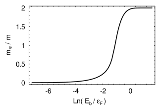
FIG. 1.: The effective mass $m_{\star}/m\/$ of the composite Bosons versus the binding energy $E_{b}/\epsilon_{F}\/$.

As was pointed out above, the mass $m_{\star}\/$ of a Cooper pair defined in such a way cannot be observed in any static measurement like the penetration depth. To discuss this, we consider the two dimensional current density

$$\boldsymbol{j}(\boldsymbol{r})=-c_{0}\frac{\delta F[\psi,\boldsymbol{A}]}{\delta\boldsymbol{A}(\boldsymbol{r})}=-2e|\psi|^{2}\frac{\hbar}{m_{\star}}\Big{(}\boldsymbol{\nabla}\phi+\frac{2e}{\hbar c_{0}}\boldsymbol{A}\Big{)}$$ (29)

which follows from (28) for a $\tau\/$-independent order parameter $\psi=|\psi|e^{i\phi}\/$. For a spatially constant magnitude $\psi_{\infty}\/$ of the order parameter, this leads immediately to the London equation

$$\boldsymbol{\nabla}\times\boldsymbol{j}(\boldsymbol{r})=-\frac{4e^{2}|\psi_{\infty}|^{2}}{m_{\star}c_{0}}\boldsymbol{h}\;.$$ (30)

As was noted above, it is only the ratio $|\psi|^{2}/m_{\star}\/$ which enters here and thus static magnetic properties are independent of the choice for $m_{\star}\/$. Specifically we consider a thin superconducting film with thickness $\delta\/$. The in-plane penetration depth $\lambda\/$ is then related to $|\psi_{\infty}|^{2}\/$ via [16]

$$L_{s}=\frac{2\,\lambda^{2}}{\delta}=\frac{m_{\star}c_{0}^{\,2}}{8\pi|\psi_{\infty}|^{2}e^{2}}\;.$$ (31)

Here we have introduced a further length $L_{s}\/$ which is the effective magnetic penetration depth in a thin film. Typically this length is of the order of one centimeter and thus for sample sizes which are smaller than that, magnetic screening may be neglected. In such a situation the difference between a charged and a neutral superfluid becomes irrelevant. A superconducting film thus exhibits a Kosterlitz-Thouless transition [17], in which the renormalized helicity modulus $\gamma(T)=\hbar^{2}|\psi|^{2}(T)/m_{\star}\/$ jumps from $2T_{c}/\pi\/$ to zero at $T_{c}\/$. Using (31) this jump translates into one for the two dimensional screening length $L_{s}\/$ of size [16]

$$\left.(L_{s}(T)\;T)\right|_{T_{c}^{\,-}}=\Big{(}\frac{\phi_{0}}{4\pi}\Big{)}^{2}=1.96\;\text{K\,cm}$$ (32)

where $\phi_{0}=hc_{0}/2e\/$ is the standard flux quantum. Consistent with our remarks above, this jump is completely universal and independent of $m_{\star}\/$, applying both to BCS- or Bose-like superconductors, provided $L_{s}\/$ is larger than the sample size and the density of vortices is low [17].

In order to define a proper superfluid density $n_{s}\/$, we consider the relation between the order parameter $\psi\/$ and the microscopic anomalous average. From Eq. (12) we have $\psi_{\rm BCS}=-g\sqrt{2c}\,\langle b\rangle\/$. Neglecting the internal d-wave structure of the order parameter and the logarithmic factor in (23), it is straightforward to see that

$$\psi_{\rm BCS}(\boldsymbol{r})\approx\xi_{b}\langle\hat{\psi}_{+1}(\boldsymbol{r})\;\hat{\psi}_{-1}(\boldsymbol{r})\rangle$$ (33)

with $\hat{\psi}_{\sigma}(\boldsymbol{r})\/$, $\sigma=\pm 1\/$ the Fermionic field operators (The factor $\ln(2\epsilon_{\Lambda}/E_{b})\/$ which is omitted in (33) diverges as $\epsilon_{\Lambda}\rightarrow\infty\/$. This is a reflection of the fact that the product of two field operators at the same point can properly defined only with a cutoff.). Since $\xi_{b}\/$ is the radius of a pair, the relation (33) shows that $|\psi_{\rm BCS}(\boldsymbol{r})|^{2}\/$ is just the areal density of pairs. This remains true even in the Bose limit where $\xi_{b}\rightarrow 0\/$ while the product $\hat{\psi}_{+1}(\boldsymbol{r})\,\hat{\psi}_{-1}(\boldsymbol{r})\/$ eventually behaves like a true Bose field operator $\hat{\psi}(\boldsymbol{r})\/$. The standard definition $n_{s}=2|\psi_{\rm BCS}|^{2}\/$ of the superfluid density can thus be applied for arbitrary coupling. By contrast, the Bose order parameter $\psi=\sqrt{m_{\star}/2m}\,\psi_{\rm BCS}\/$ coincides with $\psi_{\rm BCS}\/$ only in the strong coupling limit. For weak coupling it is given by an expression like (33) but with the interparticle spacing $k_{F}^{\,-1}\/$ instead of $\xi_{b}\/$ as the prefactor. Thus $|\psi(\boldsymbol{r})|^{2}\/$ is essentially the probability density for two Fermions with opposite spin at the same point. In the BCS limit this density is exponentially small due to the large size of a pair. The superfluid density in turn is still of order one even in weak coupling and indeed at zero temperature $n_{s}\/$ must be equal to the full density $n\/$ for any superfluid ground state in a translational system as considered here [18]. Using $n_{s}=2|\psi_{\rm BCS}(\boldsymbol{r})|^{2}\/$, the relation (32) can be rewritten in terms of a jump

$$n_{s}(T_{c}^{-})=\frac{2m}{\pi\hbar^{2}}\;T_{c}$$ (34)

of the renormalized superfluid density. The superfluid fraction $n_{s}/n\/$ therefore has a jump of order $T_{c}/T_{c}^{\,\rm Bose}\/$. Since this ratio approaches zero in weak coupling, there is a smooth crossover between the universal jump of the superfluid density in a Bose superfluid [19] and the behaviour in a strict BCS model where $n_{s}/n=2(1-T/T_{c})\/$ vanishes continuously near $T_{c}\/$ even in two dimensions. Indeed the BCS-Hamiltonian is equivalent to a model with an infinite range interaction of strength $V^{-1}\/$ for which mean field theory is exact [20]. In the following we will neglect the subtleties associated with the Kosterlitz-Thouless nature of the transition, which is anyway masked by the coupling between different CuO${}_{2}\/$-planes in real high-$T_{c}\/$ superconductors, giving a three dimensional critical behaviour near $T_{c}\/$ [21].

IV Gaussian Approximation

In order to calculate directly observable quantities from our GL functional (28), we have to determine both the critical temperature $T_{c}\/$ and the corresponding chemical potential $\mu_{c}\/$ in terms of the binding energy $E_{b}\/$. Now it is obvious that an exact evaluation of the functional integral over $\psi(\boldsymbol{r},\tau)\/$ is impossible. We will therefore use the Gaussian approximation above $T_{c}\/$, which is obtained by simply omitting the $|\psi|^{4}\/$-term. With this approximation our complete grand canonical potential $\Omega\/$ per volume takes the form

$$\Omega=\Omega_{0}+\frac{1}{\beta V}\sum\limits_{\boldsymbol{q}\,\omega_{n}}\;\ln\;gd\Big{(}-\mu_{\star}+\frac{\hbar^{2}q^{2}}{2m_{\star}}-i\,\hbar\omega_{n}\Big{)}\,.$$ (35)

The critical temperature and chemical potential then follow from the standard condition

$$\mu_{\star}(T_{c},\mu_{c})=0$$ (36)

for a bifurcation to a nonzero order parameter, and the particle number equation

$$n=-\frac{\partial\Omega}{\partial\mu}=n_{0}\\ +\,\partial_{\mu}\mu_{\star}\int\frac{d^{2}q}{(2\pi)^{2}}\;\frac{1}{\exp\big{[}\beta\big{(}-\mu_{\star}+\frac{\hbar^{2}q^{2}}{2m_{\star}}\big{)}\big{]}-1}\;.$$ (37)

Here

$$n_{0}=\frac{m}{\pi\hbar^{2}}\,\frac{\ln(1+\exp(\beta\mu))}{\beta}$$ (38)

is the number density of a free Fermion gas in two dimensions. Eq. (36) is identical with the Thouless criterion [22] for a superconducting instability, which is equivalent to the condition that the ladder approximation to the exact pair field susceptibility

$$\chi_{pair}=\int\limits_{0}^{\beta\hbar}d\tau\;\langle b_{\boldsymbol{0}}(\tau)\,b_{\boldsymbol{0}}(0)\rangle$$ (39)

diverges [23]. It is a straightforward generalization of the usual gap equation to arbitrary coupling. The number equation (37) deserves some more comments. Since we have

$$d=-\frac{1}{2}\,\partial_{\mu}a|_{\beta=\beta_{c},\mu=\mu_{c}}$$ (40)

quite generally, it is easy to see that $\partial_{\mu}\mu_{\star}=2\/$ at $\beta=\beta_{c}\/$ and $\mu=\mu_{c}\/$. Therefore Eq. (37) has the simple intuitive interpretation that the total number of particles is split into the number of free Fermions still present at $(\beta_{c},\mu_{c})\/$ plus the number of Fermions already bound together in pairs, whose mean occupation number is just the Bose distribution. Now formally this distribution function arises from the summation over the Matsubara frequencies $\omega_{n}\/$ in Eq. (35) precisely because our coefficient $a(\boldsymbol{q},\omega_{n})\/$ has been expanded only to linear order in $\omega_{n}\/$. The omission of the higher order terms in this expansion is therefore connected with neglecting scattering state contributions, which would give an additional term in Eq. (37) beyond the completely free and fully bound number of Fermions. Such a contribution is important in the three-dimensional case where true bound states exist only beyond a critical strength of the coupling [2, 7]. For our present discussion of the problem in two dimensions, however, there are only free Fermions or true bound states. Therefore there is no contribution in Eq. (37) from scattering states and one expects that the expansion of $a(\boldsymbol{q},\omega_{n})\/$ to linear order in $\omega_{n}\/$ is reliable at arbitrary strength of interaction.

There is however a rather different problem which appears in the two-dimensional case. As was discussed above, a superconducting transition exists only in the Kosterlitz-Thouless sense. This problem shows up in our Gaussian approximation, since the Bose integral in Eq. (37) diverges at $\mu_{\star}=0\/$. Now at this level of approximation this is just a reflection of the fact that $T_{c}=0\/$ for an ideal Bose gas in two dimensions, because - as pointed out above - the omission of the $|\psi|^{4}\/$-term corresponds to neglecting the repulsive interaction between the Bosons. From our analytical results (25) and (27) for $b\/$ and $d\/$, which do not contain $E_{b}\/$, it is however straightforward to calculate the effective interaction $g_{\star}\/$ for arbitrary coupling. It turns out that $g_{\star}\/$ is a monotonically decreasing function of the coupling. In the limits $\beta_{c}\mu_{c}\rightarrow\infty\/$ of a BCS-like or $\beta_{c}\mu_{c}\rightarrow-\infty\/$ of a Bose-like system, we find

$$g_{\star}=\frac{6\pi\hbar^{2}}{m}\begin{cases}\frac{\textstyle 7\zeta(3)}{\textstyle\pi^{2}}\,(\beta_{c}\mu_{c})^{2}&\text{BCS}\\ 1&\text{Bose}\end{cases}\,\,.$$ (41)

Thus, in two dimensions, there is always a finite repulsive interaction between the pairs, which is of purely statistical origin [6, 14]. In particular $g_{\star}\/$ remains finite in the Bose limit, where it arises from processes with a virtual exchange of one of the constituent Fermions in a Bose-Bose scattering process [24]. The fact that $g_{\star}\/$ is very large in the weak coupling limit is simply a consequence of the large pair size $\xi_{0}\sim\beta_{c}\epsilon_{F}\/$ (note that $\mu_{c}=\epsilon_{F}\/$ in the weak coupling limit), but does not imply that the $|\psi|^{4}\/$-term is particularly relevant in this regime. On the contrary, using the Gaussian approximation, it is straightforward to show [10] that in this limit the product $g_{\star}\langle|\psi|^{2}\rangle\/$ which effectively renormalizes the Boson chemical potential $\mu_{\star}\/$, is of order $\sqrt{E_{b}\epsilon_{F}}\/$ which is roughly $T_{c}\/$ in the weak coupling limit. For BCS-like superconductors the $|\psi|^{4}\/$-contribution is therefore irrelevant except very close to $T_{c}\/$, a fact which is well known from the standard theory of conventional superconductors. Now the finite value of $g_{\star}\/$ guarantees that even in two dimensions there is a finite critical temperature below which the superfluid density is nonvanishing. Unfortunately it is not possible to incorporate the Kosterlitz-Thouless nature of the transition in an approximate treatment of the GL functional. However considering the effectively three-dimensional structure of high-$T_{c}\/$ superconductors, this problem may be circumvented by including the motion in the direction perpendicular to the planes. A very simple method to incorporate this is provided by adding a transverse contribution $\epsilon_{\perp}\/$ to the kinetic energy by [25]

$$\frac{\hbar^{2}q^{2}}{2m_{\star}}\rightarrow\frac{\hbar^{2}q^{2}}{2m_{\star}}+\frac{\hbar^{2}q_{\perp}^{\,2}}{2m_{\perp}}\;,$$ (42)

whose average is equal to the thermal energy $\langle\epsilon_{\perp}\rangle=T\/$. Replacing the integral in Eq. (37) by

$$\int\frac{d^{2}q}{(2\pi)^{2}}\;\;\rightarrow L_{\perp}\;\,\int\frac{d^{2}q}{(2\pi)^{2}}\int\frac{dq_{\perp}}{2\pi}$$ (43)

with $L_{\perp}=2\pi/\sqrt{\langle q_{\perp}^{\,2}\rangle}\;\/$ we obtain an effectively three-dimensional system. This becomes evident by writing the contribution of the bound pairs in (37) in the form

$$n^{\prime}=\frac{m_{\star}\,\partial_{\mu}\mu_{\star}\,\sqrt{\beta}}{\pi\hbar^{2}}\,\int\limits_{0}^{\infty}d\epsilon\;\frac{\sqrt{\epsilon}}{\exp[\beta(-\mu_{\star}+\epsilon)]-1}\;.$$ (44)

The density of states is thus proportional to $\sqrt{\epsilon}\/$ as in three dimensions, making $n^{\prime}\/$ finite at $\mu_{\star}=0\/$. Although rather crude, this approximation gives a value for $T_{c}\/$ in the Bose limit, which is very close to the Kosterlitz-Thouless value for the transition temperature [17]

$$T_{c}^{KT}={0.89}\frac{\pi\hbar^{2}n}{4mk_{B}}$$ (45)

of a dilute hard core Bose gas on a lattice[26] with Boson mass $2m\/$ and number density $n/2\/$.

Using our results for the GL coefficients $a\/$, $c\/$ and $d\/$ and the replacement (44) in the number equation, we can now determine both $T_{c}\/$ and $\mu_{c}\/$ for arbitrary coupling from $\mu_{\star}=0\/$ and Eq. (37). The corresponding results are shown in Figs. 2 and 3 in units of the characteristic energy scale $\epsilon_{F}\/$ and as a function of the dimensionless effective coupling $E_{b}/\epsilon_{F}\/$. For weak coupling $E_{b}\ll\epsilon_{F}\/$, the critical temperature is monotonic in $E_{b}\/$, behaving like $T_{c}\approx\sqrt{E_{b}\epsilon_{F}}\/$. For intermediate coupling, it exhibits a maximum [6]. A similar but less pronounced behaviour is found in three dimensions, again in the Gaussian approximation [2, 7]. In a more refined self-consistent treatment [27], however, the critical temperature is a monotonically increasing function of the coupling. It is likely that the same situation also applies in two dimensions, but unfortunately there is at present no quantitative theory taking into account the repulsive interaction between the pairs in this case. In the Bose limit the transition temperature becomes independent of the original attractive interaction and is completely determined by the Boson density $n/2\/$ and the effective mass $m_{\star}\rightarrow 2m\/$. It approaches a value of about $10\%\/$ of the Fermi energy, which is likely to be an upper limit for $T_{c}\/$ in the present problem.

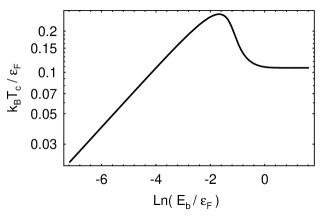
FIG. 2.: The normalized critical temperature $T_{c}\/$ versus the dimensionless coupling strength.

The chemical potential $\mu_{c}\/$ at the transition decreases monotonically from its weak coupling value $\epsilon_{F}\/$ to $-E_{b}/2\/$ in the Bose limit. It changes sign at $\ln(E_{b}/\epsilon_{F})\approx-1.1\/$, where the behaviour crosses over from BCS- to Bose-like (In Fig 3 we have supressed a small dip in $\mu_{c}\/$ around these couplings which is an artefact of the pronounced maximum in $T_{c}\/$). Apart from the chemical potential $\mu_{c}\/$, the nature of the transition can also be inferred from evaluating the number of preformed Bosons at $T_{c}\/$. This quantity, which is just half of the contribution (44) to the number equation is shown in Fig. 4. It is obvious that the nature of the phase transition changes rather quickly in a range of couplings between $\ln(E_{b}/\epsilon_{F})\approx-2\/$ and $-1\/$. For smaller couplings, the density of preformed pairs near $T_{c}\/$ is essentially negligible and binding occurs simultaneously with condensation. On the other hand, for $\ln(E_{b}/\epsilon_{F})\gtrsim-1\/$ basically all pairs are already present above $T_{c}\/$ and the transition to superconductivity is that of a true Bose system.

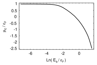
FIG. 3.: The normalized chemical potential $\mu_{c}\/$ at the critical point versus coupling.

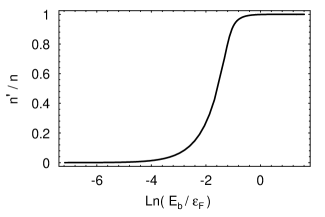
FIG. 4.: Contribution $n^{\prime}\/$ of bound pairs at the critical point to the total Fermion number density $n\/$.

V Characteristic Lengths

In the following we want to determine both the coherence length $\xi\/$ and the penetration depth $\lambda\/$ as a function of the coupling. The former is defined both above and below $T_{c}\/$ and may be obtained from the GL coefficients simply via

$$\xi^{2}=\frac{\hbar^{2}}{2m}\frac{c}{a}\;.$$ (46)

The definition of a penetration depth in a two-dimensional superconductor has been discussed in section III. Within the Gaussian approximation we may replace $|\psi_{\infty}|^{2}\/$ in (31) by $\mu_{\star}/g_{\star}\/$ which leads to

$$\lambda^{2}=\lambda_{L}^{2}\cdot\frac{bn}{4c|a|}\;.$$ (47)

Here we have introduced the bare value $\lambda_{L}\/$ of the London penetration depth defined by

$$\lambda_{L}^{2}=\frac{mc_{0}^{\,2}}{4\pi n_{3}e^{2}}$$ (48)

with $n_{3}=n/\delta\/$ the nominal three-dimensional carrier density. Note that both $\xi\/$ and $\lambda\/$ have been written in terms of the original static GL-coefficients $a,b\/$ and $c\/$, in order to stress that the characteristic lengths are independent of the normalization of $\psi\/$, i.e. the kinetic coefficient $d\/$ does not enter here. Since the coefficient $a\/$ vanishes at the transition, both $\xi\/$ and $\lambda\/$ diverge. Now in a full treatment of the GL-functional, including the $\psi^{4}\/$-term, the behaviour very close to $T_{c}\/$ in a single layer would be of the Kosterlitz-Thouless type. The correlation length would thus diverge like [17] $\ln{\xi}\sim|T-T_{c}|^{-1/2}\/$ while $\lambda^{-2}\/$ would jump from zero to a finite value below $T_{c}\/$ (see (32)). In the three-dimensional case, the behaviour very close to $T_{c}\/$ is that of a 3d XY-model with nontrivial but well known critical exponents [21]. In our Gaussian approximation this complex structure is replaced by a simple mean field behaviour. However there is a subtle point even at this level of approximation. Indeed the coefficient $a\/$ depends both on temperature and chemical potential and it is only in the strict BCS-limit, where the latter is a fixed constant equal to $\epsilon_{F}\/$. With increasing coupling, however, the chemical potential changes and thus the relevant limit close to $T_{c}\/$ is to consider $a(T,\mu(T))\/$ as $T\to T_{c}\/$. Now by using the exact relation (40), it is straightforward to show [10] that $a(T,\mu(T))\sim(T-T_{c})^{2}\/$ vanishes quadratically near $T_{c}\/$. The resulting critical exponent for the correlation length would thus be $\nu=1\/$. Indeed this is the exponent expected for an ideal Bose gas in three dimensions, to which our Gaussian approximation is effectively equivalent. Now in order to allow a comparison of our results with measured values of $\xi\/$ and $\lambda\/$, which are found to obey a mean field behaviour with $\nu=1/2\/$ except very close to $T_{c}\/$ [28], we neglect the temperature dependence of the chemical potential near $T_{c}\/$. As a result

$$a(T,\mu_{c})=a^{\prime}\cdot\frac{T-T_{c}}{T_{c}}$$ (49)

vanishes linearly near $T_{c}\/$, giving the standard mean field divergence of $\xi\/$ and $\lambda\/$. Obviously this approximation is only reliable on the weak coupling side of the transition. As we will see below, however, this is indeed the relevant regime even in high-$T_{c}\/$ superconductors. We thus expect that our results are at least qualitatively reliable for these systems. For strong coupling, the derivative $a^{\prime}\/$ of $a(T,\mu_{c})\/$ near $T_{c}\/$ vanishes like $\exp(-\beta_{c}E_{b}/2)\/$. As a result, the characteristic lengths $\xi\/$ and $\lambda\/$ would increase exponentially in the Bose limit which is unphysical however. We have therefore restricted our calculation of the GL coherence length $\xi(0)\/$ defined by

$$\xi^{2}(0)=\frac{\hbar^{2}}{2m}\frac{c}{a^{\prime}}$$ (50)

to coupling strengths $\ln(E_{b}/\epsilon_{F})\/$ smaller than about $-1\/$, where the system starts to cross over to Bose like behaviour. The corresponding result for $\xi(0)\/$ in units of $k_{F}^{-1}\/$ is shown in Fig. 5.

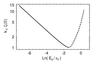
FIG. 5.: The Ginzburg-Landau coherence length $\xi(0)\/$ versus the coupling strength.

It exhibits the expected decrease of the coherence length from its weak coupling limit

$$k_{F}\xi(0)|_{\rm BCS}=\sqrt{\frac{7\,\zeta(3)}{8\pi^{2}}}\;\frac{\epsilon_{F}}{T_{c}}$$ (51)

to values of order one near the crossover regime, before it starts to rise again. As was noted above our approximations in determining $\xi(0)\/$ are no longer reliable in this regime. While in three dimensions $\xi(0)\/$ is expected to increase like $1/\sqrt{a_{B}}\;\/$ [29] with $a_{B}=2a_{F}\to 0\/$ the relevant Bose-Bose scattering length [7], the actual behaviour in two dimensions is unknown. Fortunately, however, this problem does not arise in determining the GL-parameter $\kappa=\lambda/\xi\/$ which, in two dimensions, can be expressed as

$$\kappa=\left(\frac{m}{8\pi\hbar^{2}}\cdot\frac{b\,\delta}{c^{2}r_{\rm cl}}\right)^{1/2}\;.$$ (52)

Here we have introduced the equivalent of the classical electron radius $r_{\rm cl}=e^{2}/mc_{0}^{\,2}\/$ where $m\/$ is the band mass. Since the problematic coefficient $a\/$ has dropped out in $\kappa\/$, we can use (52) to determine the GL-parameter in the whole regime between weak and strong coupling. In the BCS-limit $\kappa\/$ is exponentially small, behaving like $\kappa_{\rm BCS}\approx T_{c}/\epsilon_{F}\cdot(\delta/r_{\rm cl})^{1/2}\/$. The associated penetration depth $\lambda(0)=\sqrt{3/4}\,\lambda_{L}\/$ is thus essentially equal to the London value $\lambda_{L}\/$. By contrast, for the Bose case $\kappa\/$ approaches a constant value

$$\kappa_{\rm Bose}=\Big{(}\frac{3\delta}{r_{\rm cl}}\Big{)}^{1/2}$$ (53)

which is large compared to one, since $\delta\gg r_{cl}\/$ for realistic values of the sheet thickness $\delta\/$. The complete dependence of $\kappa\/$ in the crossover regime is shown in Fig. 6.

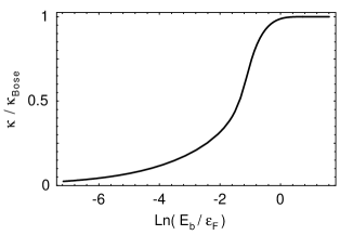
FIG. 6.: The GL parameter $\kappa\/$ versus coupling.

It is a monotonic function of the binding energy. Thus with increasing coupling there is always a transition from type I to type II behaviour in two dimensions, even for a clean superconductor with no impurities as considered here.

With these results, we are now in a position to compare our simple model with experimental values for optimally doped high-$T_{c}\/$ superconductors. Since the critical temperature is exponentially sensitive to the coupling strength and also is likely to be considerably reduced compared to our result in Fig. 2 by fluctuation effects in the crossover regime, we have refrained from taking $T_{c}\/$ as a reliable parameter for adjustment. Instead we have used the measured values of the slope of the upper critical field $H_{c_{2}}\/$ near $T_{c}\/$, which determines the GL coherence length $\xi(0)\/$ via

$$\left.\frac{dH_{c_{2}}}{d\ln T}\right|_{T=T_{c}}=\frac{\phi_{0}}{2\pi\xi^{2}(0)}\;.$$ (54)

In order to fix the dimensionless coupling strength $E_{b}/\epsilon_{F}\/$ from the measured values [30] $\xi(0)=14\,\mbox{\AA}\/$ for optimally doped YBCO ($T_{c}=92\,K\/$) and [31] $\xi(0)=24\,\mbox{\AA}\/$ for the corresponding compound BSCCO ($T_{c}=107\,K\/$), we need the in plane carrier densities $n\/$ which determine an effective value of $k_{F}=\sqrt{2\pi n}\/$ (It should be pointed out that $k_{F}\/$ is introduced here only as a measure of the carrier density. In fact due to the strong attractive interaction, the actual momentum distribution of the Fermions just above $T_{c}\/$ will be far from the standard Fermi distribution, except in the BCS limit.). The three-dimensional carrier densities in optimally doped YBCO and BSCCO are [32] $n_{3}=4\cdot 10^{21}\,cm^{-3}\/$ and [33] $n_{3}=2\cdot 10^{21}\,cm^{-3}\/$ respectively. With the corresponding values [33] $\delta=5.84\,\mbox{\AA}\/$ and $\delta=9.27\,\mbox{\AA}\/$ of the effective sheet thickness, the resulting Fermi momenta are $k_{F}=0.38\,\mbox{\AA}^{-1}\/$ for YBCO and $k_{F}=0.34\,\mbox{\AA}^{-1}\/$ for BSCCO. The dimensionless ratio $k_{F}\xi(0)=5\/$ and $8\/$ between the coherence length and the average interparticle spacing then allows us to determine the effective coupling strength. From Fig. 5 we find that $\ln(E_{b}/\epsilon_{F})\/$ is equal to $-5.1\/$ for YBCO and $-6.0\/$ for BSCCO. As Figs. 3 and 4 show, these coupling strengths describe superconductors which are still on the weak coupling side of the crossover from BCS to Bose behaviour. For instance the density of preformed Bosons at $T_{c}\/$ is less then 1% in both cases (see Fig. 4). In order to check whether our description is consistent, we determine the associated values of the GL parameter $\kappa\/$ near $T_{c}\/$. From the above values of $\delta\/$ and the band masses [32] $m=3.5\,m_{e}\/$ for YBCO and [33] $m=4.4\,m_{e}\/$ for BSCCO ($m_{e}\/$ is the free-electron mass.) we find that $\kappa_{\rm Bose}\/$ is equal to $1.5\cdot 10^{3}\/$ and $2.1\cdot 10^{3}\/$ respectively for the two compounds considered here. From Fig. 6 we thus obtain $\kappa=99\/$ and $\kappa=87\/$ for optimally doped YBCO and BSCCO. These numbers agree very well with the experimentally determined values of $\kappa\/$, which are [34] $\kappa_{\rm exp}=100\/$ and [31, 33] $\kappa_{\rm exp}=86\/$. Our simple one parameter model therefore gives a consistent quantitative description of the characteristic lengths $\xi\/$ and $\lambda\/$.

VI Conclusion

To summarize, we have studied the crossover in the superconducting transition between BCS- and Bose-like behaviour within a GL description. It has been found that optimally doped high-$T_{c}\/$ superconductors are still on the weak coupling side of this crossover, although they are certainly far away from the BCS-limit. Our microscopic model is characterized by a single dimensionless parameter, similar to the familiar BCS-Hamiltonian. While the GL functional has the standard form for arbitrary coupling its coefficients depend strongly on the coupling strength. The crossover, at least in two dimensions, is essentially identical for the s- or d-wave case. For static properties, only two of the relevant coefficients $a\/$, $b\/$ and $c\/$ are independent, since the normalization of the order parameter is arbitrary. Fixing $\xi(0)\/$ from experiment therefore leaves only one further parameter – for instance $\kappa\/$ – as an independent predicted quantity. The good agreement of $\kappa\/$ with measured values supports our conclusion that the optimally high-$T_{c}\/$ compounds are intermediate between BCS and Bose behaviour. Since the crossover regime is rather narrow, however, weak coupling theories are still a reasonable approximation for the relevant coupling strengths. This is consistent with the empirical fact that a weak coupling approach apparently works well in many cases.

Evidently there are a number of important open questions. They may be divided into two classes: the first one concerns the problem of a better and more complete treatment of our model itself. The second class is related to the problem, to which extent this model is applicable to high-$T_{c}\/$ compounds and what are the necessary ingredients for a more realistic description. Regarding our microscopic Hamiltonian as a given model, it is obvious that our treatment of the associated GL phenomenology is still incomplete. In particular the Gaussian approximation is obviously not sufficient to give a quantitatively reliable result for $T_{c}\/$ at intermediate coupling. Moreover, the behaviour of the characteristic lengths $\xi\/$ and $\lambda\/$ in the strong coupling limit is completely unknown. In order to go beyond the Gaussian approximation, it is necessary to include the pair interaction (i. e. the $|\psi|^{4}\/$-term) properly. Progress in this direction has been made in the three-dimensional case by Haussmann [27] and very recently by Pistolesi and Strinati [35]. Using a self-consistent and conserving approximation for the Green- and vertex functions, Haussmann obtained a smooth increase of $T_{c}\/$ with coupling, thus eliminating the unphysical maximum in the crossover regime found in the Gaussian approximation. This approach is rather different from our present one and requires extensive numerical work. Pistolesi and Strinati have performed an essentially analytical calculation of the correlation length $\xi_{0}\/$ at zero temperature, using a loop expansion in a functional approach similar to our present one. They have shown that the pair radius $\xi_{b}\approx\hbar/\sqrt{mE_{b}}\/$ coincides with $\xi_{0}\/$ not only in the BCS-limit, but down to values around $k_{F}\xi_{0}\approx 10\/$. Similar to our results for the GL coherence length $\xi(0)\/$ in Fig. 5, $k_{F}\xi_{0}\/$ reaches a minimum of order one in the crossover regime before it starts to rise again. Since in three dimensions the behaviour at strong coupling is that of a weakly interacting Bose gas with scattering length $a_{B}=2a_{F}\rightarrow 0\/$ [7, 24], $\xi_{0}\/$ eventually increases like $k_{F}^{\,-1}/\sqrt{k_{F}a_{B}}\/$ while $\xi_{b}\approx a_{B}\/$ approaches zero [7]. Unfortunately for the two-dimensional case, where the Boson interaction $g_{\star}\/$ is finite even at very strong coupling [6, 14], the Kosterlitz-Thouless nature of the transition makes it very difficult to improve upon the simple approximations used here. A first step in this direction was taken by Traven[36]. He showed that interactions between the pair fluctuations guarantee a nonvanishing superfluid density at finite temperature, in agreement with our arguments below Eq. (41). However there seems to be no quantitative calculation of the coherence length in a two-dimensional Bose-like regime even near zero temperature.

A different problem we want to mention here is that of the proper time dependent GL theory. Since our quantum GL functional is derived from a microscopic Hamiltonian, in principle it contains the complete information about the order parameter dynamics, at least as far as intrinsic effects are concerned. Neglecting higher order terms in the expansion in $\omega_{n}\/$, the resulting equation of motion for the order parameter in real time $t\/$ is [7]

$$d\cdot i\hbar\frac{\partial\psi(\boldsymbol{r},t)}{\partial t}=\frac{\delta F[\psi]}{\delta\psi^{\star}(\boldsymbol{r},t)}\;.$$ (55)

Due to the analytic continuation, the coefficient $d=d_{1}+id_{2}\/$ has now acquired a finite imaginary part $d_{2}>0\/$ which describes irreversible relaxation. For a better comparison with the standard literature, it is convenient to choose the conventional order parameter $\psi_{\rm BCS}=\sqrt{2c}\,z\/$, where the prefactor of the gradient term is $\hbar^{2}/4m\/$. With this choice of normalization, the kinetic coefficient $d_{1}=m^{\star}/2m\/$ is identical with the effective mass discussed in section III. It is then evident from Fig. 1 that a Gross-Pitaevskii-like dynamics where $d_{1}=1\/$, is only valid in the Bose limit, while $d_{1}\sim(T_{c}/\epsilon_{F})^{2}\/$ is exponentially small for weak coupling. Indeed for BCS-like systems it is $d_{2}\/$ which is dominant, being of order $T_{c}/\epsilon_{F}\/$ in the three-dimensional case [27]. This result reflects the fact that for weak coupling superconductors the order parameter dynamics is purely relaxing. Going beyond the BCS-limit, the associated kinetic coefficient $d_{2}\/$ has only been evaluated in three dimensions [27], where it exhibits a maximum at intermediate coupling. Its behaviour in the Bose-limit and in two dimensions in general, however, is completely unknown. Since the incorporation of scattering states in the three-dimensional case requires to go beyond the linear expansion in $\omega_{n}\/$, it is likely however, that a simple first order equation like Eq. (55) is in fact not appropriate for describing the dynamics at intermediate coupling. It is only at very low temperatures where the situation becomes simple again. Indeed from quite general arguments [37], the dynamics as $T\rightarrow 0\/$ is expected to be of the Gross-Pitaevskii form, irrespective of the strength of the coupling. Finally we mention that a proper microscopic calculation of the complex coefficient $d\/$ is relevant for understanding the Hall effect in high-$T_{c}\/$ compounds [38].

Concerning the question to which extent our model is really applicable to high-$T_{c}\/$ superconductors, it is obvious that most of the complexity of these systems is neglected here. In particular we have assumed that the normal state is characterized by a given density of effective mass Fermions with some instantaneous attractive interaction [39]. Such a system will certainly be very different from a conventional Fermi liquid for intermediate or strong coupling. Our conclusion that we are still on the weak coupling side of the crossover, with a negligible density of preformed pairs, is consistent with the phenomenology of optimally (and perhaps overdoped) high-$T_{c}\/$ superconductors, however it is certainly inappropriate for the underdoped cuprates. Indeed these systems exhibit a gap far above $T_{c}\/$ which may be interpreted in terms of preformed Bosons. A GL description of underdoped compounds was very recently developed by Geshkenbein, Ioffe and Larkin [40]. Assuming that Bosons form far above $T_{c}\/$ only in parts of the Fermi surface and coexist with unpaired Fermions through $T_{c}\/$, they obtain a reasonable description of the phenomenology of certain underdoped materials. This behaviour is quite different from that obtained in our model, which completely neglects any effects of the Coulomb repulsion and band structure. It is obvious that for a quantitative description of high-$T_{c}\/$ superconductors both Coulomb correlations and band structure effects have to be included, which requires to use lattice models. They provide a quantitative description of these complex systems at least in the normal state and allow the calculation of microscopic properties like spectral functions, etc [41]. Unfortunately with these models it still seems impossible to really explain how d-wave superconductivity arises from the strongly spin and charge correlated normal state. As a result, effective models like the negative-U Hubbard model are often used to discuss microscopic properties of high-$T_{c}\/$ compounds [42, 43]. Our present approach is more phenomenological, starting from a model in which all microscopic details are neglected except for the fact that we have a strong pairing interaction in a system of Fermions with given density. The advantage of such an approach is that it allows a simple calculation of the relevant lengths $\xi\/$ and $\lambda\/$ and quantities following from that like the critical fields. The fact that the resulting GL theory gives a consistent description of optimally doped cuprates indicates that at least at this level the microscopic details are not relevant. Certainly our results supporting this view are quite limited so far and it is necessary to investigate this further. Since the coefficients of the GL functional near $T_{c}\/$ are quite generally determined by the properties in the normal state, an interesting future direction would be to see whether superconducting properties below $T_{c}\/$ can quantitatively be obtained from the GL functional by properly incorporating the anomalous behaviour in the normal state.

- [1] A. J. Leggett, in Modern Trends in the Theory of Condensed Matter, edited by A. Pekalski und J. Przystawa (Springer, Berlin, 1980).
- [2] P. Nozières and S. Schmitt-Rink, J. Low Temp. Phys. 59, 195 (1984).
- [3] M. Randeria, in Bose-Einstein Condensation, edited by D. Snoke and S. Stringari (Cambridge University Press, 1994).
- [4] D. J. Scalapino, Phys. Rep. 250, 329 (1995).
- [5] J. Annett, N. Goldenfeld and A. J. Leggett, in Physical Properties of High Temperature Superconductors, Vol. 5, edited by D. M. Ginsberg (World Scientific, New Jersey, 1996).
- [6] M. Drechsler and W. Zwerger, Ann. der Phys. 1, 15 (1992).
- [7] C. A. R. Sá de Melo, M. Randeria and J. R. Engelbrecht, Phys. Rev. Lett. 71, 3202 (1993).
- [8] B. Mühlschlegel, in Path Integrals and their Applications in Quantum, Statistical, and Solid State Physics, edited by G. J. Papadopoulos und J. T. Devreese (Plenum Press, New York, 1977).
- [9] M. Sigrist and K. Ueda, Rev. Mod. Phys. 63, 239 (1991).
- [10] S. Stintzing, PhD thesis, Ludwig-Maximilians-Universität München 1996, unpublished.
- [11] E. P. Gross, J. Math. Phys. 4, 195 (1963).
- [12] M. Randeria, J.-M. Duan and L.-Y. Shieh, Phys. Rev. B 41, 327 (1990).
- [13] P. G. de Gennes, Superconductivity of Metals and Alloys (Addison-Wesley, Redwood City, 1989)
- [14] W. Zwerger, in Proceeedings of the Fourth International Conference on Path Integrals from meV to MeV, edited by H. Grabert, A. Inomata, L. S. Schulman and U. Weiss (World Scientific, Singapore, 1992).
- [15] L. S. Schulman, Techniques and Applications of Path Integration (Wiley, New York, 1981), Chap. 27.
- [16] B. I. Halperin and D. R. Nelson, J. Low Temp. Phys. 36, 599 (1979).
- [17] P. Minnhagen, Rev. Mod. Phys. 59, 1001 (1987).
- [18] A. J. Leggett, Physica Fennica 8, 125 (1973).
- [19] D. R. Nelson and J. M. Kosterlitz, Phys. Rev. Lett. 39, 1201 (1977).
- [20] B. Mühlschlegel, J. Math. Phys. 3, 522 (1962).
- [21] H. Keller and T. Schneider, Int. J. Mod. Phys. B 8, 487 (1994).
- [22] D. J. Thouless, Ann. of Phys. 10, 553 (1960).
- [23] A. Tokumitu, K. Miyake and K. Yamada, Phys. Rev. B 47, 11988 (1993).
- [24] R. Haussmann, Z. Phys. B 91, 291 (1993).
- [25] V. P. Gusynin, V. P. Loktev and I. A. Shovkovyi, Sov. Phys. JETP 80, 1111 (1995).
- [26] In the continuum the result (45) is modified by a double logarithmic factor, which is neglected here however, see D. S. Fisher and P. C. Hohenberg, Phys. Rev. B 37, 4936 (1987).
- [27] R. Haussmann, Phys. Rev. B 49, 12975 (1994).
- [28] S. Kamal, D. A. Bonn, N. Goldenfeld, P. J. Hirschfeld, R. Liang and W. N. Hardy, Phys. Rev. Lett. 73, 1845 (1994).
- [29] X.-G. Wen and R. Kan, Phys. Rev. B 37, 595 (1988).
- [30] U. Welp, W. K. Kwok, G. W. Crabtree, K. G. Vandervoort and J. Z. Liu, Phys. Rev. Lett. 62, 1908 (1989).
- [31] I. Matsubara, H. Tanigawa, T. Ogura, H. Yamashita and M. Kinoshita, Phys. Rev. B 45, 7414 (1992).
- [32] K. Semba, T. Ishii and A. Matsuda, Phys. Rev. Lett. 67, 769 (1991).
- [33] D. R. Harshman and A. P. Mills, Jr, Phys. Rev. B 45, 10684 (1992).
- [34] L. Krusin-Elbaum, A. P. Malozemoff, Y. Yeshurun, D. C. Cronemeyer and F. Holtzberg, Phys. Rev. B 39, 2936 (1989).
- [35] F. Pistolesi and G. C. Strinati, Phys. Rev. B 53, 15168 (1996).
- [36] S. V. Traven, Phys. Rev. Lett. 73, 3451 (1994).
- [37] M. Stone, Int. J. Mod. Phys. B 9, 1359 (1995).
- [38] For a phenomenological discussion see A. T. Dorsey, Phys. Rev. B 46, 8376 (1992).
- [39] For a treatment of the strong coupling limit for systems with a retarded interaction in terms of Eliashberg theory see G. Varelogiannis and L. Pietronero, cond-mat/9507072.
- [40] V. B. Geshkenbein, L. B. Ioffe and A. I. Larkin, Phys. Rev. B 55, 3173 (1997).
- [41] G. Dopf, J. Wagner, P. Dieterich, A. Muramatsu and W. Hanke, Phys. Rev. Lett. 68, 2082 (1992).
- [42] M. Randeria, N. Trivedi, A. Moreo and R. T. Scalettar, Phys. Rev. Lett. 69, 2001 (1992).
- [43] R. Micnas, M. H. Pedersen, S. Schafroth, T. Schneider, J. J. Rodríguez-Núñez and H. Beck, Phys. Rev. B 52, 16223 (1995).