[

Luttinger theorem for a spin-density-wave state

Abstract

We obtained the analog of the Luttinger relation for a commensurate spin-density-wave state. We show that while the relation between the area of the occupied states and the density of particles gets modified in a simple and predictable way when the system becomes ordered, a perturbative consideration of the Luttinger theorem does not work due to the presence of an anomaly similar to the chiral anomaly in quantum electrodynamics.

]

One of the key open problems in the study of high-$T_{c}$ superconductors is the shape and the area of the electronic Fermi surface near half-filling. Photoemission studies [1] performed near optimal doping have demonstrated that the area enclosed by the Fermi surface is large, and for a doping concentration $x$, constitutes a fraction $(1-x)/2$ of the area of the Brillouin zone, just as for free fermions. This is consistent with the Luttinger theorem which states that in any conventional Fermi liquid, the area enclosed by the Fermi surface does not change due to an interaction between fermions. On the other hand, similar experiments on underdoped materials have shown no evidence of a Fermi surface crossing for momenta far from the zone diagonal [2]. These data are consistent with the idea that the Fermi surface evolves with decreasing doping towards a small hole Fermi surface consisting of four pockets centered at $(\pm\pi/2,\pm\pi/2)$. The existence of such a Fermi surface in the paramagnetic phase would imply a violation of the Luttinger theorem.

To consider a possible violation of the Luttinger theorem in a system with strong magnetic fluctuations, one first needs to understand how this theorem is modified when the system acquires a long-range magnetic order. This is the issue which we address in this paper. We show that there are several subtleties which emerge already on the mean-field level. In particular, a naive perturbative approach yields incorrect results because of a hidden anomaly which requires a proper regularization.

We begin with a brief consideration of the Luttinger theorem for a conventional Fermi liquid [3]. The number of particles $N$ can be expressed through the single particle Green function $G_{k}(\omega)$ of the interacting electrons as

$$N=-i~{}{\rm Tr}\sum_{k}~{}\lim_{t\rightarrow+0}\int\frac{d\omega}{(2\pi)}G_{k}(\omega)e^{i\omega t},$$ (1)

where ${\rm\ Tr}$ implies a summation over spin projections. Using the obvious relation for $G$ and the self-energy $\Sigma$, $G_{k}(\omega)=~{}\partial\log{G_{k}^{-1}(\omega)}/\partial\omega+G_{k}(\omega)\partial\Sigma_{k}(\omega)/\partial\omega$, one can rewrite Eq.(1) as $N=I_{1}-I_{2}$ where

$$I_{1} = -i~{}{\rm Tr}\sum_{k}~{}\int_{-\infty}^{\infty}\frac{d\omega}{(2\pi)}~{}\frac{\partial}{\partial\omega}\log G_{k}^{-1}(\omega),$$ (2)

$$I_{2} = i~{}{\rm Tr}\sum_{k}~{}\int_{-\infty}^{\infty}\frac{d\omega}{(2\pi)}G_{k}(\omega)~{}\frac{\partial}{\partial\omega}\Sigma_{k}(\omega).$$ (3)

In Ref.[3], Luttinger and Ward (LW) argued that $I_{2}=0$ to all orders in perturbation theory around free fermions. Their consideration is based on a functional $Y=-i~{}{\rm Tr}~{}\sum_{k}~{}\int d\omega/(2\pi)~{}Y_{k}(\omega)$ determined by the variational equation

$$\delta Y=-i~{}{\rm Tr}~{}\sum_{k}~{}\int\frac{d\omega}{2\pi}~{}\Sigma_{k}(\omega)~{}\delta G_{k}(\omega).$$ (4)

This variational equation allows one to re-express $I_{2}$ as an integral of a full derivative:

$$I_{2}=-i~{}{\rm Tr}\sum_{k}~{}\int_{-\infty}^{\infty}\frac{d\omega}{(2\pi)}\frac{\partial Y_{k}(\omega)}{\partial\omega}.$$ (5)

LW gave a recipe how to obtain the functional $Y_{k}(\omega)$ order by order in a diagrammatic perturbation theory. The perturbative $Y_{k}(\omega)$ is free from singularities and vanishes at large frequencies. Obviously, in this situation $I_{2}=0$. (We however will demonstrate below that $I_{2}$ may be finite due to nonperturbative effects). The term $I_{1}$ also contains a full derivative over frequency and, apparently, should vanish for similar reasons. However, its calculation requires care as $\log G$ is a non-analytic function of frequency in the upper half-plane. A careful consideration shows that due to a nonanalyticity, $I_{1}$ turns out to be finite:

$$I_{1}=\frac{1}{2\pi i}~{}{\rm Tr}\sum_{k}\log\frac{G_{k}^{-1}(\mu+i0)}{G_{k}^{-1}(\mu-i0)},$$ (6)

where $\mu$ is the chemical potential of the interacting electrons. It then follows that

$$N=I_{1}={\rm Tr}~{}\sum_{k}\Theta(E_{k}-\mu),$$ (7)

where $E_{k}$ is the quasiparticle energy, and the $\Theta$-function counts the states inside the Fermi surface. This is the Luttinger theorem for a conventional Fermi liquid. It states that the number of states enclosed by the Fermi surface is equal to the number of particles $N$.

The Luttinger relation can be easily extended to the case when the system develops a long-range magnetic order. Consider for definiteness a 2D spin-fermion model which describes a system of propagating fermions with dispersion $\epsilon_{k}$ coupled to localized spins $S_{q}$ by an exchange interaction [4, 5]: ${\cal H}_{int}=g\sum_{{\bf q,k},\alpha,\beta}c_{\alpha,k+q}^{\dagger}{\vec{\sigma}}_{\alpha\beta}c_{\beta,k}~{}{\vec{S}_{q}}$. Here $\sigma^{i}$ are the Pauli matrices, and the localized spins are described by their dynamical spin susceptibility, $\chi(q,\omega)$. For simplicity, we assume that there are no other interactions, i.e., for $g=0$ one deals with free fermions. In the antiferromagnetically ordered phase one of the components of ${\vec{S}}$ acquires a nonzero expectation value $<S_{q}^{z}>=<S^{z}>\delta_{q,Q}$. In the mean-field spin-density-wave (SDW) theory, the interaction term reduces to $\Delta c_{\alpha,k+Q}^{\dagger}\sigma_{\alpha\alpha}^{z}c_{\alpha,k}$, where $\Delta=g<S^{z}>$. Problems of this kind are most conveniently described in a matrix formalism. In the presence of the SDW order, the electronic spectrum can be obtained from the $4\times 4$ matrix

$$G_{k}^{-1}(\omega)=\left[\begin{array}[]{cc}\omega-{\bar{\epsilon}}_{k}&\Delta\,\,\sigma_{z}\\ \Delta\,\,\sigma_{z}&\omega-{\bar{\epsilon}}_{k+Q}\end{array}\right]\text{,}$$ (8)

where ${\bar{\epsilon}}_{k}=\epsilon_{k}-\mu$, and $\mu$ is the actual, $\Delta$-dependent chemical potential. For the purpose of comparison with the paramagnetic phase we will keep using the original Brillouin zone rather than the magnetic one. Then, for each $k$ one gets two solutions ${\bar{E}}_{k}^{~{}\pm~{}}$ $=({\bar{\epsilon}}_{k}+{\bar{\epsilon}}_{k+Q})/2~{}\pm~{}[\Delta^{2}+(({\bar{\epsilon}}_{k}-{\bar{\epsilon}}_{k+Q})/2)^{2}]^{1/2}$ which satisfy ${\bar{E}}_{k}^{\pm}={\bar{E}}_{k+Q}^{\pm}$ . The relations (1),(3) between $N$ and the single particle Green’s function still hold in the ordered state, with the only modification that ${\rm Tr}$ now acts on $4\times 4$ matrices. In a mean-field approximation the $I_{2}$ term vanishes identically, and hence $N=I_{1}$. A substitution of Eq.(8) into Eq.(6) yields $N=\sum_{k}\left(\Theta({\bar{E}}_{k}^{+})+\Theta({\bar{E}}_{k}^{-})\right).$ Subtracting this relation from the total number of states in the Brillouin zone, $N_{BZ}$, one finally obtains

$$x=S_{hole}-S_{double},$$ (9)

where $x\equiv 1-N/N_{BZ}$ is a hole doping concentration, while $S_{hole}$ and $S_{double}$ are fractions of the Brillouin zone occupied by hole pockets (${\bar{E}}^{\pm}>0$) and doubly occupied electronic states (${\bar{E}}^{\pm}<0$), respectively. Eq.(9) is the Luttinger relation for the ordered SDW phase. It has been derived here in a mean-field approximation, but Eq.(9) should also hold in the presence of fluctuations due to an interaction between fermions, simply because the effect of the spin ordering is completely absorbed into the matrix formulation of the LW functional $Y$.

We now give the physical interpretation of the Luttinger relation for the ordered state. For this, we fix the doping concentration at some small but finite level and follow the Fermi surface evolution with increasing $\Delta$. For $\Delta=0$, the Fermi surface has the form shown in Fig 1a - it is centered at $(\pi,\pi)$ and encloses an area which is slightly larger than half of the Brillouin zone, in accordance with the conventional Luttinger theorem, Eq. (7).

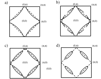
FIG. 1.: Schematic evolution of the Fermi surface with the gap $\Delta$ in the ordered SDW phase with electron hopping to nearest ($t$) and next-nearest($t^{\prime})$ neighbors on a square lattice. We set $t^{\prime}=-0.2t$. The dashed line indicates the boundary of the magnetic Brillouin zone.

Switching on an infinitesimally small $\Delta$ doubles the unit cell in real space. As a result, extra pieces of the Fermi surface appear because a Fermi surface crossing at $k$ necessarily implies one at $k+Q$ (Fig. 1b). The subsequent evolution of the Fermi surface proceeds as is shown in Fig. 1c,d. For sufficiently large $\Delta$, the doubly occupied electron states disappear, and the Fermi surface consists of just four small hole pockets centered at $(\pi/2,\pi/2)$ (see Fig. 1d). The total area enclosed by the pockets is small and scales as $x$ in agreement with Eq.(9).

So far, the LW argumentation works perfectly. However, the matrix formalism cannot be extended to the paramagnetic phase. We now discuss another, complimentary approach to the ordered state in which one does not explicitly introduce a condensate of $S^{z}$ but instead obtains the SDW form of the electronic spectrum by introducing an exchange of $\delta-$functional longitudinal spin fluctuations: $\chi_{l}(q,\Omega)=(\Delta/g)^{2}\delta(\Omega)\delta(q-Q)$. This approach is advantageous as it can be applied to the paramagnetic phase - one just has to substitute the $\delta-$functional longitudinal susceptibility by the one with a finite spin-spin correlation length  [5, 6]. In the spin-fluctuation formalism, the full Green’s function does not have a matrix structure, but there appears a self-energy due to spin-fluctuation exchange. To the lowest order in $\Delta^{2}$,

$$\Sigma_{k}(\omega)=\Delta^{2}G_{k+Q}^{(0)}(\omega)=\frac{\Delta^{2}}{\omega-{\bar{\epsilon}}_{k+Q}},$$ (10)

where $G_{k}^{(0)}(\omega)=(\omega-{\bar{\epsilon}}_{k})^{-1}$ is the Green’s function of free electrons. For the $\delta-$functional form of $\chi_{l}$ this is in fact an exact result - the higher order terms in $\Sigma$ are absent due to a Ward identity [5]. The full Green’s function then takes the form

$$G_{k}(\omega)=\frac{\omega-{\bar{\epsilon}}_{k+Q}}{(\omega-{\bar{E}}_{k}^{+})(\omega-{\bar{E}}_{k}^{-})}.$$ (11)

Not surprisingly, it coincides with the diagonal part of the matrix $G$ defined by Eq.(8). At the same time, the $I_{1,2}$ terms are not the same in the matrix and the diagonal formalisms. Moreover, the self-energy in (10) has a singular frequency dependence. We therefore have to reexamine the argument that $I_{2}=0$. To begin with, we first observe that $I_{1}$ alone does not yield the right expression for $N$. Indeed, it follows from Eqs.(3,11) that

$$I_{1}=~{}2\sum_{k}\left(\Theta({\bar{E}}_{k}^{+})+\Theta({\bar{E}}_{k}^{-})-\Theta({\bar{\epsilon}}_{k+Q})\right).$$ (12)

For large $\Delta$, $I_{1}=2(1-x)N_{BZ}$ in clear disagreement with Eq.(9). This implies that $I_{2}$ should be finite. Observe that the numerator in (11) also contributes to $I_{1}$.

To calculate $I_{2}$, we use Eq.(5) which relates $I_{2}$ to the LW functional $Y$. This functional can be straightforwardly obtained by performing the functional integration of the self-energy $\Sigma$ over $G_{k}(\omega)$. To do this, we first have to re-express $\Sigma$ in terms of the full Green’s functions. This can be done either directly, by substituting $G_{k+Q}^{(0)}(\omega)$ in Eq.(10) in terms of $G$, or diagrammatically, by rewriting the self-energy as $\Sigma_{k}(\omega)=\Delta^{2}G_{k+Q}(\omega)\Gamma_{k,k+Q}(\omega)$, and collecting diagrams for the full vertex $\Gamma$ order by order in the perturbative expansion, each time using full propagators $G$ for the internal fermionic lines. It turns out, however, that the results of the two approaches are different, because there exists a range of frequencies where the perturbative expansion is not convergent. Indeed, a formal summation of the perturbation series for the self-energy yields $\Sigma_{k}^{pert}(\omega)=2\Delta^{2}G_{k+Q}(\omega)/\left(1+\sqrt{1+4\Delta^{2}G_{k}(\omega)G_{k+Q}(\omega)}\right)$. On the other hand, the use of an exact relation between bare and full Green’s functions yields

$$\Sigma_{k}(\omega)=\frac{2\Delta^{2}G_{k+Q}(\omega)}{1\pm\sqrt{1+4\Delta^{2}G_{k}(\omega)G_{k+Q}(\omega)}}.$$ (13)

Here the upper and lower signs should be used when $|y|<1$ and $|y|>1$, respectively, where $y=\Delta^{2}G_{k}^{(0)}(\omega)G_{k+Q}^{(0)}(\omega)$. Clearly, the perturbative and exact expressions for the self-energy coincide only for $|y|<1$, i.e., when the perturbative expansion is convergent.

We now show that due to the difference between $\Sigma$ and $\Sigma^{pert}$, the actual $I_{2}$ is finite, while the perturbative approach yields $I_{2}=0$ to all orders in $\Delta$. Indeed, performing the integration over the Green’s function in Eq.(4) and using Eq.(13) for $\Sigma$, we find

$$Y_{k}(\omega) = \frac{1}{2}\Bigg{[}-\log G_{k}(\omega)\pm\sqrt{1+4\Delta^{2}G_{k}(\omega)G_{k+Q}(\omega)}$$ (14)

$$\pm \frac{1}{2}\log\Bigg{(}\frac{\sqrt{1+4\Delta^{2}G_{k}(\omega)G_{k+Q}(\omega)}-1}{\sqrt{1+4\Delta^{2}G_{k}(\omega)G_{k+Q}(\omega)}+1}\Bigg{)}\Bigg{]}.$$ (15)

After simple manipulations, $Y_{k}(\omega)$ can be rewritten as

$$Y_{k}(\omega)=\frac{1}{4}\log\frac{G_{k}^{(0)}(\omega)G_{k+Q}^{(0)}(\omega)}{G_{k}^{2}(\omega)}+Y_{k}^{reg}(\omega),$$ (16)

where $Y_{k}^{reg}(\omega)$ is a regular function of frequency. We now substitute the functional $Y_{k}(\omega)$ into Eq.(5) for $I_{2}$. The integral in (5) contains a full derivative but, similarly to what we previously obtained in the calculation of $I_{1}$, it does not vanish. The point is that due to a nonanaliticity, the logarithmic term in Eq.(16) does not allow one to reduce the integral to just the values of $Y_{k}(\omega)$ at the limits of integration. Doing the same manipulations as with $I_{1}$, we obtain

$$I_{2}=\sum_{k}\left(\Theta({\bar{E}}_{k}^{+})+\Theta({\bar{E}}_{k}^{-})-2\Theta({\bar{\epsilon}}_{k})\right)\;.$$ (17)

Collecting now the $I_{1}$ and $I_{2}$ contributions to $N$ we indeed reproduce the correct result, Eq.(9). It is essential, however, that $I_{2}$ is finite (e.g., for large $\Delta$, $I_{2}=(1-x)N_{BZ}$ ). On the other hand, we have checked that if we use the perturbative expression for $\Sigma$, we obtain $I_{2}$ in the form of an integral of a full derivative over frequency of a regular function $Y_{k}^{pert}(\omega)$ which vanishes at $\omega=\pm\infty$. In this case, the integral is indeed equal to zero.

To make this point clearer and also to discuss some analogy with field theory, we now compute $I_{2}$ directly by substituting the expressions for the full Green’s function and the full self-energy into Eq.(3). We find

$$I_{2} = -2i\Delta^{2}\sum_{k}\int\frac{d\omega}{2\pi}~{}(\omega-\bar{{\epsilon}}_{k+Q}+i\delta_{\omega})^{-1}$$ (19)

$$\times[(\omega-\bar{E}_{k}^{+}+i\delta_{\omega})(\omega-\bar{{E}}_{k}^{-}+i\delta_{\omega})]^{-1},$$

where $\delta_{\omega}=\delta\ sgn\omega$. In a perturbation theory, one assumes that $\Delta$ is small and expands $I_{2}$ in powers of $\Delta$: $I_{2}=\sum_{n=1}^{\infty}\Delta^{2n}I_{2}^{(n)}$, where $I_{2}^{(n)}$ is evaluated at $\Delta\equiv 0$. Performing this expansion in (19) and integrating over frequency, we find

$$I_{2}^{(n)}=\sum_{k}~{}~{}\frac{\Theta({\bar{\epsilon}}_{k})-\Theta({\bar{\epsilon}}_{k+Q})}{({\bar{\epsilon}}_{k}-{\bar{\epsilon}}_{k+Q})^{2n}}.$$ (20)

Clearly, $I_{2}^{(n)}=0$ for all $n$ by symmetry: the summation over $k$ in (20) goes over the full Brillouin zone while the function changes sign when $k$ and $k+Q$ are interchanged. In principle, the very fact that $I_{2}^{(n)}=0$ to all orders in perturbation theory does not exclude an exponential dependence of $I_{2}$ on $1/\Delta^{2}$. However, we explicitly computed $I_{2}$ numerically using Eq.(17) and found that $I_{2}\propto\Delta^{2}$ at small $\Delta$, i.e., $I_{2}$ possesses a regular dependence on the expansion parameter. For $t^{\prime}=-0.2t$ and $\mu=-0.69t$, we found $I_{2}\approx-0.63\Delta^{2}/t^{2}$.

We now show that the reason for the discrepancy between the explicit and perturbative calculations lies in the fact that $lim_{\Delta\rightarrow 0}\;I_{2}/\Delta^{2}\neq I_{2}^{(1)}$ where $I_{2}^{(1)}$ is given by Eq.(20). Indeed, examine the form of $I_{2}^{(1)}$ before the frequency integration is performed. We have

$$I_{2}^{(1)}=-2i\sum_{k}\int\frac{d\omega}{2\pi}\frac{1}{(\omega-{\bar{\epsilon}}_{k+Q}+i\delta_{\omega})^{2}~{}(\omega-{\bar{\epsilon}}_{k}+i\delta_{\omega})}.$$

We see that the integrand in $I_{2}^{(1)}$ contains a double pole at $\omega=\bar{\epsilon}_{k+Q}$, i.e., the frequency integral is in fact linearly divergent. This divergence, however, does not show up in the final result as changing $k$ to $k+Q$, one finds the same divergence, but with opposite sign. Compare now this formula with the exact (nonperturbative) form for $I_{2}$, Eq.(19). We see that the inclusion of the SDW self-energy correction into the Green’s function splits the double pole at $\omega={\bar{\epsilon}}_{k+Q}$ into two closely located poles at $\omega={\ \bar{\epsilon}}_{k+Q}$ and $\omega=\bar{E}_{k}^{-}$ for $\epsilon_{k}>\epsilon_{k+Q}$, or $\omega=\bar{E}_{k}^{+}$ for $\epsilon_{k}<\epsilon_{k+Q}$. For most of the Brillouin zone, both poles lie in the same half-plane. However, for $\bar{\epsilon}_{k}\bar{\epsilon}_{k+Q}<\Delta^{2}$, the poles at ${\bar{\epsilon}}_{k+Q}$ and, e.g., $\bar{E}_{k}^{+}$ are located in different half-planes in which case the frequency integration yields a contribution which is absent in the case $\Delta=0$. The region in momentum space where this new contribution exists is very narrow, its area is of the order of $\Delta^{2}$. However, everywhere in this region, the denominator in $I_{2}$ is also of the order of $\Delta^{2}$ as $\bar{E}_{k}^{+}-{\bar{\epsilon}}_{k+Q}\sim\Delta^{2}$. As a result, the additional contribution to $I_{2}/\Delta^{2}$ remains finite as $\Delta\rightarrow 0$. To calculate this contribution, we transformed the summation over momenta into the integration over energies and integrated over a narrow region in ${\ \bar{\epsilon}}_{k+Q}:|{\bar{\epsilon}}_{k+Q}|<\Delta^{2}/|{\bar{\epsilon}}_{k}|$. We then obtained $I_{2}/\Delta^{2}$ in the form of a one-dimensional integral over $d{\bar{\epsilon}}_{k}$:

$$lim_{\Delta\rightarrow 0}\;I_{2}/\Delta^{2}=\frac{1}{4\pi^{2}t|t^{\prime}|}\int^{{\bar{\epsilon}}^{max}}_{{\bar{\epsilon}}^{min}}\frac{d{\bar{\epsilon}}_{k}}{{\bar{\epsilon}}_{k}W({\bar{\epsilon}}_{k})},$$ (21)

where $W({\bar{\epsilon}}_{k})=((1+a)^{2}-b^{2})(b^{2}-4a))^{1/2},~{}a=({\bar{\epsilon}}_{k}-2|\mu|)/(8|t^{\prime}|),~{}b={\bar{\epsilon}}_{k}/(4t),~{}{\bar{\epsilon}}^{max}=4|\mu|/(1+(1-|\mu t^{\prime}|/t^{2})^{1/2}),~{}{\bar{\epsilon}}^{min}=2(4t^{\prime}-\mu)/(1+2|t^{\prime}|/t)<0$. Performing the one-dimensional integration numerically, we found for $t^{\prime}=-0.2t$ and $\mu=-0.69t$, $I_{2}\approx-0.63\Delta^{2}/t^{2}$ which is exactly the same result that we obtained using Eq.(17). We have checked that this equivalence also holds for other values of $t^{\prime}$ and $\mu$. Notice that contrary to naive expectations, the integration in Eq.(21) is not confined to a region near the points where the Fermi surface crosses the magnetic Brillouin zone boundary (hot spots). These points correspond to ${\bar{\epsilon}}_{k}=0$ in the integrand in Eq.(21). In fact, if we substitute $W({\bar{\epsilon}}_{k})$ by $W(0)$, we would obtain a very different $I_{2}$ which for some $t^{\prime}$ even possesses the wrong sign.

The anomaly which gives rise to a finite value of $I_{2}$ is very similar to the chiral anomaly in quantum electrodynamics [7]. In both cases, we have an integral which apparently vanishes by symmetry, but contains a hidden linear divergence. Performing a regularization, one gets rid of the divergence but simultaneously brakes the symmetry. In our case, the proper regularization is achieved by performing all computations at a small but finite $\Delta$, i.e., keeping the symmetry broken at all stages of the calculations. After regularization, the double pole gets split into two poles, and there appears an extra contribution from the region, where the poles are in different half-planes. This extra contribution turns out to be finite because the smallness of the phase space is fully compensated by the smallness of the energy denominator.

Finally, let us discuss how the opening of the gap $\Delta$ influences the chemical potential $\mu$. Combining Eqs.(9) and (5), we find $I_{2}=2\sum_{k}[\Theta(\epsilon_{k}-\mu_{\Delta=0})-\Theta(\epsilon_{k}-\mu)]$. Clearly, the fact that $I_{2}$ is finite implies that $\mu\neq\mu_{\Delta=0}$. For large $\Delta$, $|\mu|\approx\Delta\gg|\mu_{\Delta=0}|$.

In summary, in this paper we obtained the Luttinger relation for the antiferromagnetically ordered state. For a formalism where one does not introduce an antiferromagnetic order parameter, we have demonstrated that the perturbative derivation of the Luttinger theorem breaks down because of a hidden anomaly which needs to be regularized. We found similarities between this phenomenon and the chiral anomaly in quantum electrodynamics.

The present paper only considers the magnetically ordered state. It was recently argued by two of us [5] that $I_{2}$ remains finite even in the paramagnetic phase if the spin-fermion coupling strength exceeds some threshold value. This argument is consistent with the idea of small hole pockets in heavily underdoped cuprates. A more detailed study of the possible violation of the Luttinger theorem in the paramagnetic phase is clearly called for.

It is our pleasure to thank all colleagues with whom we discussed this issue. This research was supported by NSF DMR-9629839 (for A. C. and D. M.), and by the German-Israel Foundation - GIF (for A. D. and A. F.). A. Ch. is an A.P. Sloan fellow. A. F. is supported by the Barecha Fund Award.

REFERENCES

- [1] K. Gofron et al., Phys. Rev. Lett. 73, 1885 (1995); D.S. Dessau et al., ibid 71, 2781 (1993), J. Ma et al., Phys. Rev. B 51, 9271 (1995).
- [2] D.S. Marshall et al., Phys. Rev. Lett 76, 4841 (1996); H. Ding et al., Nature 382, 51 (1996); S. LaRosa et al, preprint, (1996).
- [3] J.M. Luttinger and J.C. Ward, Phys. Rev 118, 1417 (1960), J.M. Luttinger, Phys. Rev 119,1153 (1960).
- [4] P. Monthoux and D. Pines, Phys. Rev. B 47, 6069 (1993); Phys. Rev. B 50, 16015 (1994).
- [5] A.V. Chubukov, D.K. Morr, and K.A. Shakhnovich, Phil. Mag. B 74, 563 (1996); A.V. Chubukov and D.K. Morr, Phys. Rep., to be published (1997).
- [6] A.P. Kampf and J.R. Schrieffer, Phys. Rev. B 42, 7967 (1990).
- [7] S.B. Treiman, R. Jackiw, and D.J. Gross, in Lectures on Current Algebra and Its Applications, (Princeton University Press, Princeton, 1972).