Liouville Field Theory of Fluctuating Loops

Abstract

Effective field theories of two-dimensional lattice models of fluctuating loops are constructed by mapping them onto random surfaces whose large scale fluctuations are described by a Liouville field theory. This provides a geometrical view of conformal invariance in two-dimensional critical phenomena and a method for calculating critical properties of loop models exactly. As an application of the method, the conformal charge and critical exponents for two mutually excluding Hamiltonian walks on the square lattice are calculated.

PACS numbers: 05.50.+q, 11.25.Hf, 64.60.Ak, 64.60.Fr

The study of critical phenomena in two dimensions has led to a rather remarkable interplay between statistical mechanics and field theory. The picture that has emerged portrays critical fluctuations in a variety of systems as being described by a conformal field theory (CFT), i.e., a quantum field theory invariant under local scale (conformal) transformations. This view has proven very fruitful as it has answered many questions pertaining to two-dimensional phase transitions. For example, by studying the representations of the Virasoro algebra, which is the algebra of conformal transformations, we have come to understand why critical exponents in two-dimensions are typically rational numbers [1]. Lists of possible critical exponents appear here in very much the same way one discovers the quantization of angular momentum by studying the representations of the algebra of rotations.

Progress in understanding two-dimensional critical phenomena using CFT’s has largely come about by classifying these field theories and associating them with the scaling limits of specific microscopic lattice models [1, 2]. Still a fundamental practical question remains: Given a lattice model how does one go about constructing a conformal field theory of its scaling limit? It is this question, limited in scope to lattice models of fluctuating loops [3], which is addressed here. Since most canonical two-dimensional models can be recast as loop models [4], the results we find are general in nature, and provide a geometrical view of criticality and conformal invariance in two-dimensions. In particular, we find that CFT’s of loop models can be constructed explicitly via a mapping of the loop model to a model of a fluctuating surface. The basic idea is to think of loops as contour lines of a random surface; the field theory which describes the large-scale fluctuations of this surface is a conformally invariant Liouville field theory.

Liouville field theory provides a general framework for calculating correlation functions in CFT’s; this is the well known Coulomb gas representation pioneered by Dotsenko and Fateev [5]. The central result of this paper is the discovery that different terms in the Liouville action, some of which were originally introduced on formal grounds, have a concrete geometrical interpretation in loop models. Furthermore, the coupling constants, most notably the effective stiffness of the surface $K$, are fixed by geometry, thus providing a method for calculating critical properties of loop models exactly. To illustrate this we calculate the conformal charge and critical exponents for a new loop model defined on the square lattice. For vanishing loop weights this model defines a new universality class of Hamiltonian walks; these are self-avoiding random walks that visit all the sites of the lattice. Hamiltonian walks have been used in the past to model configurational statistics of polymer melts [6].

a Loop models

Given a two-dimensional lattice ${\cal L}$ a loop configuration ${\cal G}$ is defined by a set of loops, which are closed self-avoiding walks along the bonds of ${\cal L}$. The partition function is $Z=\sum_{\cal G}\exp[-\beta H({\cal G})]$, where $\beta H({\cal G})$ is the reduced loop-Hamiltonian.

As remarked in the introduction, many two-dimensional models can be recast as loop models. For example, in the Potts model one arrives at a loop model description by considering the graphs generated by the high-temperature expansion of the partition function [4]; in the $O(n)$ model, the partition function takes the form of a loop model once integration over the spin degrees of freedom is carried out [7]. Here we focus our attention on fully packed loop (FPL) models whose allowed configurations ${\cal G}$ satisfy the constraint that every vertex of the lattice is visited by a loop, and

$$\beta H({\cal G})=\sum_{i=1}^{n_{f}}\mu_{i}N_{i}({\cal G})\;.$$ (1)

is the loop Hamiltonian. Here we have allowed for $n_{f}$ flavors of loops; $n_{i}=\exp(-\mu_{i})$ is the loop weight, and $N_{i}$ is the number of loops of flavor $i$. In the allowed configurations ${\cal G}$ only different flavored loops can cross. An important example of an FPL model is provided by the critical Q-state Potts model, which can be mapped to an FPL model on the (oriented) square lattice with $n_{f}=1$ and $n=\sqrt{Q}$ [2]. Recent interest in FPL models [8, 9, 10, 11] has been sparked by their close relation to the problem of Hamiltonian walks: from the Bethe ansatz solution of the FPL model on the honeycomb lattice exact critical properties of Hamiltonian walks on a non-oriented lattice were obtained for the first time [9].

In order to illustrate the general relation between loop models and Liouville field theories, we calculate the exact conformal charge and critical exponents for the two-flavor ($n_{f}=2$) fully packed loop model (FPL²) on the square lattice, with loop weights $n_{1}=n_{2}=n>0$. The two loop flavors of the model will be denoted black and grey, in accord with Fig. 1a; the possible vertex configurations of the FPL² model are shown in Fig. 1b. The allowed loop configurations are the same as in the dimer-loop model [12], and the FPL model on the square lattice [11], the difference being in the loop weights. For the dimer loop model $n_{1}=2$, $n_{2}=1$, while the FPL model generalizes this to $n_{1}=n>0$, $n_{2}=1$. Obviously the FPL and FPL² models share a common point: $n=1$. We will show later that for $n=1$ there is excellent agreement between the numerical results of Ref. [11] and our exact expressions.

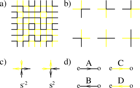
FIG. 1.: The two-flavor fully packed loop (FPL²) model on the square lattice: a) loop configuration ${\cal G}$; b) allowed vertex configurations; c) two vertex configurations of oriented loops (of 24 total) and their weights – $s=\exp(i\pi e_{0}/4)$; d) mapping to the coloring model – “e” and “o” denote sites on the even and odd sublattice of the square lattice.

It is instructive to look at the $n\to 0$ ($\mu\to\infty$) and $n\to\infty$ ($\mu\to-\infty$) limits of the FPL² model. From Eq. (1) we infer that in the first limit configurations with one black and one gray loop are selected. These self-avoiding walks are Hamiltonian and they can be thought of as a model of two mutually repelling species of polymers in the melt. Later we will show that this model defines a new universality class of Hamiltonian walks. In the limit $n\to\infty$ the selected loop configurations maximize the number of loops, each being of minimum length four. In this case the model has a finite correlation length ($\xi$), measured by the average loop size, while in the case of Hamiltonian walks the correlation length obviously diverges with system size. Later we will argue that at $n=2$ a transition occurs between a critical phase ($\xi\to\infty$) and a long range ordered one (finite $\xi$).

b Liouville field theory

To calculate the critical properties of a loop model we construct a random surface for which the loops are contour lines. This construction can be broken up into three steps, which are illustrated here for the FPL² model.

First we orient all the loops; for every loop configuration ${\cal G}$ this gives $2^{N_{1}({\cal G})+N_{2}({\cal G})}$ oriented-loop configurations. In order to recover the proper loop weights ($n$) every left/right turn of the oriented black and grey loops is assigned a weight $\lambda=\exp(\pm{\rm i}\pi e_{0}/4)$; if the loop does not make a turn, $\lambda=1$ is the appropriate weight (see Fig. 1c). On the square lattice the difference between the number of left and right turns that a closed loop makes is $\pm 4$, so the $\lambda$’s along a loop will combine to give a weight of $\exp(\pm{\rm i}\pi e_{0})$, depending on the loop orientation. After summing over the two possible orientations, the correct loop weight

$$n=e^{{\rm i}\pi e_{0}}+e^{-{\rm i}\pi e_{0}}=2\cos(\pi e_{0})$$ (2)

is recovered.

There is an important caveat to the above construction. Namely, if we define the loop model on a cylinder, then the loops that wind around the cylinder are weighted incorrectly, with $n=2$, since the number of left and right turns for these loops is equal. To correct this a boundary term is introduced in the effective action for the FPL² model – $S_{b}$ in Eq. (3) [2].

Second, we map configurations of oriented loops to configurations of a microscopic height ${\bf z}=(z_{1},z_{2},z_{3})$ which defines a two dimensional interface in five dimensions; the black and grey loops are contour lines of projections of ${\bf z}$ along different directions. The microscopic heights are defined at the centers of the plaquettes of ${\cal L}$ in the following way. The difference in ${\bf z}$ between two neighboring plaquettes depends on the flavor and direction of the bond that they share, and is given by one of four vectors (also referred to as colors): ${\bf A}=(-1,1,1)$, ${\bf B}=(1,1,-1)$, ${\bf C}=(-1,-1,-1)$, or ${\bf D}=(1,-1,1)$; Fig. 1d. This height mapping is the same as the one for the four-coloring model on the square lattice [13].

Third, we coarse grain the microscopic height. We view the configurations of ${\bf z}$ as consisting of flat domains over which ${\bf z}$ is averaged so as to obtain a coarse grained height ${\bf h}$ [13]. The partition function of the loop model which incorporates only the large scale fluctuations of ${\bf h}$ can be written as a functional integral $\int\!{\cal D}{\bf h}\exp(-S)$, where $S$ is the effective action. $S$ can be broken up into three terms,

$$S = S_{e}+S_{b}+S_{w}$$ (3)

$$S_{e} = \frac{K}{2}\int\!\!d^{2}{\bf x}\;[(\partial_{1}{\bf h})^{2}+(\partial_{2}{\bf h})^{2}]$$ (4)

$$S_{b} = \frac{{\rm i}}{4\pi}\int\!\!d^{2}{\bf x}\;({\bf E}_{0}\cdot{\bf h})R$$ (5)

$$S_{w} = \int\!\!d^{2}{\bf x}\;w({\bf h})\;,$$ (6)

each having a simple geometrical interpretation:
i) $S_{e}$ describes the elastic fluctuations of the interface. Its form, namely the fact that the elasticity is given by a single stiffness constant $K$, is fixed by the symmetries of the loop model: four-fold rotations of the lattice, translations in height space, and cyclic permutations of the colors [12, 14].
ii) $S_{b}$ is the above mentioned boundary term that corrects the weights of loops that wind around a cylinder [2]. $R$ is the scalar curvature, which for a particular choice of coordinates on the cylinder is the difference of two delta functions centered at the two ends. The term $S_{b}$ therefore has the effect of placing vertex operators $\exp(\pm{\rm i}{\bf E}_{0}\cdot{\bf h})$ at the boundaries of the cylinder. In the Coulomb gas representation vertex operators are associated with electric charges, and ${\bf E_{0}}$ is referred to as the background charge [5]. In the chosen normalization for the color-vectors ${\bf E}_{0}=(-\pi e_{0},0,0)$.
iii) $S_{w}$ ensures the correct weight of loops in the bulk. Namely, as mentioned earlier, the loops of the FPL² model are contours of ${\bf h}$, and if the only bulk term in $S$ were $S_{e}$ then the two loop orientations would be equivalent – $S_{e}$ equally weights a step up and a step down in height. This is inconsistent with $n\neq 2$ and an additional bulk term is necessary.

It is important to note that a similar construction, leading to $S_{e}$ and $S_{b}$, has been used previously by many authors, and it goes under the name: Coulomb gas approach to critical phenomena [7, 15]. The important difference here is the inclusion of the loop-weight term $S_{w}$. The presence of this term in the effective action fixes the value of $K$, which in the traditional Coulomb gas approach would remain unknown, only to be determined by an exact value of some critical exponent, typically derived from a Bethe ansatz solution of the model. For the cases where Bethe ansatz solutions do exist (e.g., Potts models, $O(n)$ models) we have checked that the geometrical approach developed here reproduces the same value of the stiffness (“renormalized coupling”) [14, 10].

Microscopically, the operator $w({\bf h}({\bf x}))$ in $S_{w}$ generates the vertex weights $\lambda({\bf x})$ in Fig. 1d: $\lambda=\exp(-w)$. This operator can be written as $w({\bf h}({\bf x}))=\frac{{\rm i}}{16}\>{\bf E}_{0}\cdot{\bf Q}({\bf x})$ [14], where ${\bf Q}({\bf x})$ is the cross-staggered operator defined in Ref. [13]; it is a vector valued function of the colors around the site ${\bf x}\in{\cal L}$. ${\bf Q}({\bf x})$ is periodic in height space and it can be expanded in a Fourier series of vertex operators $\exp({\rm i}{\bf G}\cdot{\bf h}({\bf x}))$; the vectors ${\bf G}$ lie in the lattice which is reciprocal to the lattice of height periods, and they are the electric charges in the Coulomb gas representation. The magnetic charges on the other hand form the lattice of height periods, and they are associated with vortex configurations of the height with topological charge ${\bf b}$ [13].

In the long-wavelength limit we only keep the most relevant vertex operator appearing in the Fourier expansion of ${\bf Q}({\bf x})$; this is the operator with the smallest scaling dimension. The scaling dimension of a general operator with an electro-magnetic charge $[{\bf G},{\bf b}]$ is given by [5]:

$$x[{\bf G},{\bf b}]=\frac{1}{4\pi K}\>{\bf G}\cdot({\bf G}-2{\bf E}_{0})+\frac{K}{4\pi}\>{\bf b}^{2}$$ (7)

Therefore, the loop weight term in Eq. (3) can be written as:

$$S_{w}=Ce_{0}\int\exp({\rm i}{\bf G}_{Q}\cdot{\bf h}({\bf x}))\>d^{2}{\bf x}$$ (8)

where $C$ is a constant independent of $n$, and ${\bf G}_{Q}=(-\pi,0,\pi)$ minimizes $x[{\bf G},0]$.

For $n\leq 2$ the effective action $S$, with $S_{w}$ given by Eq. (8), describes a Liouville field theory with imaginary couplings; $w({\bf h})$ is the so-called Liouville potential. In order for $S$ to describe a conformal field theory it is necessary that $w({\bf h})$ is a marginal operator, i.e., $x[{\bf G}_{\bf Q},0]=2$ [5]. Moreover, if $S$ is a CFT then $w({\bf h})$ is exactly marginal, and the coupling $Ce_{0}$ does not flow under renormalization. The exactly marginal operator $w({\bf h})$ gives rise to a line of fixed points, which is the aforementioned critical phase of the loop model. For $n>2$ the parameter $e_{0}$ in Eq. (2) becomes pure imaginary. From Eq. (7), and the assumption that $K$ increases with $n$, it follows that in this case the scaling dimension of $w({\bf h})$ is necessarily less then two – it is relevant. Therefore, under renormalization $n\to\infty$, and the loop model is in the ordered phase.

In the Coulomb gas representation of two-dimensional critical models the Liouville potential defines the so-called screening charges, which were originally introduced on formal grounds – to ensure the non-vanishing of the four-point correlation functions [5]. In the case of loop models we have uncovered a geometrical interpretation of the Liouville potential: it enforces the correct weighting of oriented loops by making the two orientations inequivalent.

The assumption that $w({\bf h})$ is exactly marginal – which we refer to as the conformal ansatz – has a simple geometrical interpretation. Namely, the loop weight ($n=2\cos(\pi e_{0})$) is thermodynamically conjugate to the number of loops ($N$), and its non-renormalizability implies that the number of large loops, which are responsible for the long-wavelength fluctuations of the height, does not change under renormalization. In this form the conformal ansatz is closely analogous to the hypothesis often made for critical percolation, that the number of spanning clusters is of order one, which in turn leads to hyperscaling [16].

c Exact results

The conformal ansatz implies $x[{\bf G}_{\bf Q},0]=2$, and from Eq. (7) we calculate the exact value of the stiffness

$$K=\frac{\pi}{4}\>(1-e_{0})\;;$$ (9)

for further convenience we define the parameter $g\equiv 4K/\pi$. Using Eqs. (2) and (9) for the coupling constants of the effective field theory (Eq. (3)), we can calculate the conformal charge and the critical exponents of the loop model along the critical line $n\leq 2$.

The conformal charge is [5]:

$$c=3-12\>\frac{{\bf E}_{0}^{2}}{4\pi K}=3-12\>\frac{(1-g)^{2}}{g}\;.$$ (10)

For $n=2$ and $n=1$, $g=1$ and $g=2/3$, and consequently $c=3$ and $c=1$; $c=3$ is the conformal charge of the four-coloring model which can be mapped to the $n=2$ FPL² model [13], while $c=1$ is the known conformal charge of the equal-weighted six-vertex model [2], which is equivalent to the $n=1$ FPL² model [11].

In the limit of Hamiltonian walks ($n\to 0$, $g=1/2$) we find $c=-3$. This differs from the conformal charge for a single Hamiltonian walk on the honeycomb ($c=-1$ [9]) or the square ($c=-1.00(1)$ [11]) lattice, and we conclude that the FPL² model defines a new universality class of self-avoiding random walks. This is also confirmed by the critical exponents, which we calculate next.

The most commonly studied operators in the context of loop models are the so called string (“watermelon”) operators whose two-point correlation function gives the probability of having $m$ loop segments propagating between two points on the lattice [17]; here we focus on string operators associated with black loops only. In the Coulomb gas representation of the FPL² model these operators are associated with mixed electric and magnetic charges: $[(-e_{0}\pi/2,0,e_{0}\pi/2),(-2k,0,-2k)]$ is the charge for the $m=2k$ string operator, while $[(-e_{0}\pi,0,0),(-2k,-2,2k-2)]$ for $m=2k-1$ [14]. These charges can be determined microscopically by mapping the string configurations to vortex configurations of the height; an analogous analysis for the FPL model on the honeycomb lattice can be found in Ref. [10]. From Eq. (7) we can calculate the scaling dimensions of the string operators,

$$x_{2k} = \frac{g}{2}k^{2}-\frac{(1-g)^{2}}{2g}$$ (11)

$$x_{2k-1} = \frac{g}{2}(k^{2}-k+1)-\frac{(1-g)^{2}}{g}\;.$$ (12)

The dimensions associated with an even number of strings are the same as those found for the FPL model on the honeycomb lattice, while the odd ones are new. In particular, in the Hamiltonian limit ($n\to 0$, $g=1/2$) we find $x_{1}=-1/4$. This, via standard scaling relations [9], leads to a prediction for the exponent $\gamma=1-x_{1}=5/4$, which describes the scaling of the number of walks with the number of steps (bonds traversed). This value of $\gamma$ is different from the ones found for a single walk on the honeycomb ($\gamma=1$ [9]) and the square lattice ($\gamma\approx 1.0444$ [11]), confirming once again that the FPL² model defines a new universality class of Hamiltonian walks.

For $n=1$ the FPL² model coincides with the FPL model of Batchelor et al. [11]. For this value of $n$, $g=2/3$, and $x_{1}=1/6$ and $x_{2}=1/4$, while the numerical transfer matrix results quoted in Ref.[11] are $x_{1}=0.1667(1)$ and $x_{2}=0.2500(1)$. Furthermore Batchelor et al. found numerical evidence for the relation $x_{3}=x_{1}+g$, which we find to be satisfied exactly.

In conclusion, we have shown that the conformal field theory associated with the scaling limit of a lattice loop-model can be constructed by mapping it to a random surface. The loops appear as contour lines of a surface whose long wavelength fluctuations are described by a Liouville field theory. The remarkable feature of loop models is that the couplings in the field theory are completely fixed by geometry thus leading to exact results for their critical properties.

The conformal ansatz, which is equivalent to the statement that the number of large loops does not change with length scale, is central to the whole construction, and it leads to a physical interpretation of the Dotsenko-Fateev screening charges [5]. The validity of this ansatz has been confirmed for loop models for which an exact solution exists (e.g., Potts models, $O(n)$ models) [14, 10]. In order to show this explicitly a renormalization group which takes into account the extended nature of loops will have to be developed. This remains an interesting open question.

Enlightening discussions with J. Cardy, J. deGier, C.L. Henley, G. Huber, J.B. Marston, B. Nienhuis, V. Pasquier and T. Spencer are acknowledged. I am particularly indebted to J. Cardy who alerted me to the relation between the Liouville potential and the screening charges, and to C.L. Henley for pointing out the relation between the loop weight and the number of large loops. It is also a pleasure to acknowledge the hospitality of T. Spencer and the Institute for Advanced Study, where part of this work was completed. This work was supported by the NSF through grant No. DMR-9357613.

REFERENCES

- [1] A.A. Belavin, A.M. Polyakov, and A.B. Zamolodchikov, Nucl. Phys. B241, 333 (1984).
- [2] J. Cardy in Fields, Strings, and Critical Phenomena, E. Brezin and J. Zinn-Justin eds. (Nort Holland 1990).
- [3] S.O. Warnaar, B. Nienhuis, and K.A. Seaton, Phys. Rev. Lett. 69, 710 (1992). S.O. Warnaar and B. Nienhuis, J. Phys. A 26, 2301 (1993).
- [4] R.J. Baxter, Exactly Solved Models in Statistical Mechanics (Academic Press, 1982).
- [5] Vl.S. Dotsenko and V.A. Fateev, Nucl. Phys. B240, 312 (1984), and Nucl. Phys. B251, 691 (1985).
- [6] J. des Cloizeaux and G. Jannink, Polymers in Solution (Oxford University Press, 1990).
- [7] B. Nienhuis, in Phase Transitions and Critical Phenomena, edited by C. Domb and J.L. Lebowitz (Academic, London, 1987), Vol. 11.
- [8] H. W. J. Blöte and B. Nienhuis, Phys. Rev. Lett. 72, 1372 (1994).
- [9] M. T. Batchelor, J. Suzuki and C. M. Yung, Phys. Rev. Lett. 73, 2646 (1994).
- [10] J. Kondev, J. deGier, and B. Nienhuis, J. Phys. A 29, 6489 (1996).
- [11] M.T. Batchelor et al., J. Phys. A 29, L399 (1996).
- [12] R. Raghavan, S. L. Arouh, and C. L. Henley, to appear in J. Stat. Phys.
- [13] J. Kondev and C.L. Henley, Phys. Rev. B52, 6628 (1995).
- [14] J. Kondev, to be submitted to Nuclear Physics B.
- [15] P. Di Francesco, H. Saleur, and J.-B. Zuber, J. Stat. Phys. 49, 57 (1987).
- [16] A. Coniglio in Physics of Finely Devided Matter, N. Boccara and M. Daoud eds. (Springer-Verlag, 1985).
- [17] B. Duplantier, Phys. Rep. 184, 222 (1989).