Enhanced magnetic fluctuations in doped spin-Peierls systems: a single-chain model analysis

Abstract

We analyze by means of real space Renormalization Group (RG) as well as by exact diagonalizations the properties of a single-chain model of a doped spin-Peierls system, where a major role is played by the localized moments created by the impurities. We are able to follow analytically the RG flow, which allows us to determine the relevant cross-over temperatures. In particular, we find an enhancement of magnetic correlations due to disorder, coexisting with an underlying dimerization, in an intermediate temperature range below the spin-Peierls critical temperature and above the coherence temperature of a regular array built by those localized moments (so-called soliton bandwidth). The possible relevance of these results to the doped inorganic spin-Peierls compound CuGeO₃ is discussed.

I Introduction

The behavior of spin-Peierls systems in the presence of disorder has recently attracted considerable interest in the light of the intriguing properties of the inorganic CuGeO₃ compound. The pure compound is a quasi-one dimensional material, in which the interchain couplings in the two directions perpendicular to the chains are estimated to be 10% and 1% of the intrachain coupling. At at temperature $T_{SP}\simeq 14K$, there is a structural transition, below which the CuO₂ chains dimerize and a gap in the spin excitation spectrum opens[1]. The properties below $T_{SP}$ are reasonably well described by a dimerized Heisenberg chain, with an additional next-nearest neighbour exchange coupling[2].

If few percent of Cu is substituted by magnetic (Ni[3]) or non magnetic (Zn[4, 5, 6]) ions, or, if Ge is replaced by Si[7, 8], besides the structural transition, which still occurs close to 14K, a second transition is detected at $T_{N}\simeq 2\div 4K$, which has been identified as a Néel antiferromagnetic transition. The staggered magnetic moment with 4% of Zn is estimated of the order of 0.2$\mu_{B}$[5].

The simplest explanation of the appearence of a Néel phase upon such a weak doping, is that already the pure compound is quite close to a transition from a spin liquid phase, with a gap in the excitation spectrum, to an antiferromagnetic state, with gapless spin wave excitations. Then, one could imagine that doping effectively reduces the dimerization, or increases the interchain coupling, so that the system is pushed quickly in the magnetically ordered phase. Within this picture, one would represent the disordered system still as a homogeneous system but with modified parameters, and the enhancement of the magnetic fluctuations would be simply due to the critical quantum fluctuations. Notice that a dimerized exchange is not incompatible with a Néel order in more than one dimension, which explains the coexistence of dimerization and magnetic ordering. However, in our opinion, this explanation is not fully consistent with the experiments. A detailed discussion, including also a review of existing results, is postponed to the conclusion section.

Therefore we believe that something else has to be invoked to explain why the spin-liquid phase of the pure CuGeO₃ is so unstable upon doping. In this paper we introduce and study another mechanism of enhancement of the antiferromagnetic fluctuations, which is purely due to disorder, exists also in a single chain, and can not be represented by a homogeneous system with modified parameters. Essentially, we will assume that, at low doping, the impurities release spin-1/2 solitonic excitations, which, however, are not free to move but get trapped in the vicinity of the impurities by interchain correlations[9, 10]. Antiferromagnetic fluctuations can then be established since a coupling between these localized spins is generated by the polarization of the spin-singlet background. However, one would naively disregard the effects of these magnetic fluctuations, since they are supposed to appear at an energy/temperature scale $T_{*}$ of the order of the spin-wave bandwith which would be obtained if these localized spins formed a regular lattice (soliton lattice bandwidth). This scale is proportional to the spin-Peierls gap with a prefactor exponentially small in the ratio of the average distance between the impurities to the soliton width. At 2% Zn-doping, with the estimated soliton width of 13.6 lattice spacings[11], this prefactor would be of order 0.025, while it would be 0.16 at 4% doping. Since at 2% Zn-doping $T_{N}\simeq 0.28T_{SP}$[5], it would be hard to believe that these localized spins have something to do with the antiferromagnetism. We will show that this naive conclusion is not correct when these solitons are randomly distributed. In fact, as a consequence of disorder, sensible magnetic correlations will form well above $T_{*}$. Therefore, this effect may in principle play a role in the establishment of antiferromagnetism. Notice that this source of enhancement of magnetic fluctuations is not incompatible with the previously discussed scenario, rather it favours the approach to the critical point separating the spin liquid from the magnetically ordered phase. As we are going to discuss, we believe that there are evidences that these disorder-induced fluctuations play a role in these materials, especially at low doping.

The paper is organized as follows. In section II we will introduce the model and discuss some existing results. In section III we will introduce the renormalization group approach which we use to study the model, and start the analysis, which will be further improved in section IV with the calculation of the spin-spin correlation function. In section V we present some numerical results which support the renormalization group analysis. Section IV is devoted to exact diagonalizations of small clusters, the interchain coupling being treated in mean field. The conclusions are given in section VII.

II The model

The Hamiltonian which we consider in the absence of impurities is simply that of a dimerized Heisenberg chain

$$\hat{H}=\sum_{i}(1+\delta(-1)^{i})\left(S^{x}_{i}S^{x}_{i+1}+S^{y}_{i}S^{y}_{i+1}+\Delta S^{z}_{i}S^{z}_{i+1}\right),$$ (1)

where $\delta$ is the strength of the dimerization. As we said, to correctly describe the CuGeO₃ compound, one should include a next nearest neigbour coupling. However, for our purposes, this is not really important. We assume that one impurity releases one spin-1/2 solitonic excitation, connecting regions of different dimerization parity[12]. The role of the interchain coupling is to provide a confining potential to the soliton, which will be trapped within some distance from the impurity[9] (as well as to enlarge the soliton width[13]). Moreover, the weak link connecting the impurity nearest neighbors (which would be generated by virtual hoppings into and out from the impurity site, as well as by a next-nearest neighbor exchange) is approximated to be equal to the weak bonds in (1). This approximation is valid if one is interested really in what happens close to the middle of the spin-Peierls gap. Therefore, for a finite number $n_{imp}$ of randomly distributed impurities, the effective model will be assumed to consist of a squeezed chain with $n_{imp}$ sites less, described by the same Hamiltonian Eq.(1), but in the presence of randomly distributed domain walls. Their number will be $\leq n_{imp}$, since we can not exclude that pairs of solitons recombine. This amounts to take a site dependent $\delta(i)$, which takes alternatively two values $\pm\delta$, jumping from one to the other at the (random) position of the antiphase walls. If we assume no correlation between the impurities, then the distance $r$ between two consecutive domain walls is distributed according to a Poisson law

$$P(r)=n{\rm e}^{-(r-a)n}\theta(r-a),$$ (2)

where $n$ is the concentration of domain walls, and $a$ is of the order of the lattice spacing. The XY version of this model [$\Delta=0$ in Eq.(1)], has been recently studied in the continuum limit ($a\to 0$) in Ref.[14]. In this reference, exact expressions of the density of states as well as of several thermodynamic quantities have been derived. These results are supposed to give a good qualitative description up to the isotropic point [$0\leq\Delta\leq 1$ in Eq.(1)], since, as discussed in Refs.[15] and [16], the spin anisotropy in a disordered chain does not play the same crucial role as in the absence of disorder. In this paper, we will study the low energy (lower that the spin-Peierls gap) behavior of the spin-isotropic model by means of the real space Renormalization Group (RG) originally introduced by Dasgupta and Ma[17] to cope with random spin chains, and further extended by Fisher[16]. We will show that this approach reproduces the exact results obtained in the XY limit in Ref.[14], thus proving the unimportance of the spin anisotropy for $0\leq\Delta\leq 1$. In addition, by this technique it is also possible to calculate the spin-spin correlation functions, which were not calculated in Ref. [14], being not easily accessible by the method used in that paper.

A Effective low energy model

We start our analysis by building an effective low energy model which should describe the Hamiltonian (1) below the spin Peierls gap, and for low doping. In this regime, most of the spins are frozen into singlets apart from the spin-1/2 solitons localized around the domain walls. Two consecutive solitons are coupled by an exchange which we assume of the form

$$J(r)=\phi_{0}{\rm e}^{-r\phi_{0}},$$ (3)

where $r$ is the distance between the two, which is distributed according to (2), and $1/\phi_{0}$ is the soliton width. We have choosen units in which the energy has the dimension of an inverse length. Therefore the resulting low energy model describes a random Heisenberg model where spins are randomly distributed on a chain according to the law (2), and coupled by the exchange constants (3). This model should give a correct description of (1) at energies/temperatures smaller than $\phi_{0}$, and for $n\ll\phi_{0}$ (the solitons should not overlap too much), and can be analysed by the RG technique of Ref.[16], as we are going to show in the following sections. A similar low energy picture has been proposed in Ref.[18] on the basis of an exact diagonalization of a realistic model for CuGeO₃, although limited to small clusters. By analyzing their data, the authors of that reference have concluded that the random Heisenberg model is indeed a good description for the low energy excitations. Here, given for granted this low energy picture, we analyze some possible consequences, which can be useful for a comparison with experimental data as well as a guiding line for further numerical studies.

It is now worthwhile to realize that the antiferromagnetic correlations in the squeezed chain do not simply translate into oscillations with wave vector $Q=\pi/a$ in the original chain. This is due to the presence of the impurities which change one sublattice into the other, since the coupling across the impurity site is antiferromagnetic. For instance, if in the squeezed chain a correlation function oscillates like $\cos(Qx)$, in the original chain it will oscillate like $\cos[Q(x-N(x))]$, where $N(x)$ is the number of impurities in that interval. For randomly distributed impurities, after the averaging, this behavior will transform into $\cos(Qx){\rm e}^{-2n_{i}x}$, where $n_{i}$ is the impurity concentration. Therefore, within this single chain model, we can not describe a true Néel long range order. For that, we would need to properly take into account the interchain coupling. A first attempt is discussed in section IV.C, where we calculate the susceptibility to a staggered (in the original chain, not in the squeezed one) magnetic field. However, for the purpose of describing how disorder enhances magnetic fluctuations, without pretending to push the analysis up to the AF transition, the single chain model we study is sufficient.

To conclude, we notice that the XY version of this model is equivalent to a tight-binding Hamiltonian for spinless fermions at half filling with random hopping integrals. This model has been studied quite a lot in connection with the Anderson localization, for its intriguing properties. A detailed analysis was carried out by Eggarter and Riedinger[19]. They showed, quite generally, that the density of states has a Dyson singular behavior at the chemical potential $\rho(\epsilon)\sim 1/|\epsilon\ln^{3}\epsilon|$, and that the localization length diverges logarithmically $\lambda(\epsilon)\sim|\ln\epsilon|$. However, they did not discuss the consequences of these singularities in the correlation functions. This analysis was partially carried out by Gogolin and Mel’nikov[20] using the Berezinskii diagram technique. They showed, for instance, that, although one dimensional, this system has a finite conductivity. However, their approach is quite complicated and does not provide a simple interpretation of the low energy behavior. On the contrary, the RG analysis carried out by Fisher for the spin model is, physically, more simple, and, once translated in the fermion language of the tight-binding model, provides not only a simple low energy picture but also many new results, as for instance the zero temperature power law decay of the average density-density correlation function. We have verified these predictions numerically in the tight-binding model, as we are going to discuss in section V.

III Renormalization of the bond distribution

We start giving a very short introduction to the RG transformation. Then, as a warm up exercise, we will calculate the renormalization of the probability distribution of the bond exchange-couplings.

The RG transformation consists in successive eliminations of the most strongly coupled pairs of spins, by projecting out the Hilbert space onto the subspace where those pairs are frozen into singlets. The cut-off energy which is rescaled downwards in the course of the renormalization procedure is the strength of the strongest bond $\Omega=\max\{J\}$. Therefore, going from $\Omega$ to $\Omega-\delta\Omega$, amounts to project out all those pairs of spins which are coupled by an exchange of value $\Omega$. This operation generates an effective bond between two spins separated by a projected pair. If, for instance, at the energy scale $\Omega$, the coupling between spins 2 and 3 is $J_{2,3}=\Omega$, then the projection onto the subspace in which those spins are frozen into a singlet generates a coupling between the neigbouring spins 1 and 4, given by $J_{1,4}=J_{1,2}J_{3,4}/J_{2,3}$. The decimation scheme becomes more and more valid in the course of the scaling procedure, as one verifies by the flowing of the bond probability distribution.

In our particular case, as previously discussed, we will consider a chain where spins are randomly distributed in such a way that the distribution of distances $r$ between two consecutive spins is given by (2). The bond connecting two consecutive spins at distance $r$ has a strength given by (3). Following Fisher, we define $\Gamma=\ln(\phi_{0}/\max\{J\})$, and a new variable $\zeta=-\Gamma+\ln(\phi_{0}/J(r))$. The recursion relation for the $\zeta$-variable is quite simple in the above decimation scheme. In fact, in our previous example, where the sites 2 and 3 are decimated, a coupling between sites 1 and 4 is generated, such that $\zeta_{1,4}=\zeta_{1,2}+\zeta_{3,4}-\zeta_{2,3}=\zeta_{1,2}+\zeta_{3,4}$, being $\zeta_{2,3}=0$. We also define a scaling variable $\eta=\zeta/\Gamma$. At our RG starting point, $\Gamma_{0}=\phi_{0}a$, $\eta=(r-a)/a$, and the initial $\eta$ distribution is

$\displaystyle Q(\eta,\Gamma_{0})=\frac{\Gamma_{0}n}{\phi_{0}}\exp{\left(-\frac{n\Gamma_{0}}{\phi_{0}}\eta\right)}\theta(\eta).$

With these notations, the RG scaling equation for $Q$ is[16]

$$\Gamma\frac{\partial Q}{\partial\Gamma}=Q+(1+\eta)\frac{\partial Q}{\partial\eta}+Q(0,\Gamma)\int_{0}^{\eta}d\eta^{\prime}Q(\eta^{\prime},\Gamma)Q(\eta-\eta^{\prime},\Gamma).$$ (4)

We search for a solution of (4) of the form: $Q(\eta,\Gamma)=\bar{f}(\Gamma)\exp{(-\bar{f}(\Gamma)\eta)}\theta(\eta)$, with $\bar{f}$ independent of $\eta$. At the starting point $\bar{f}(\Gamma_{0})=na$. The equation of motion of $\bar{f}(\Gamma)$ is

$$-\Gamma\frac{\partial\bar{f}(\Gamma)}{\partial\Gamma}=-\bar{f}(\Gamma)+\bar{f}^{2}(\Gamma),$$ (5)

whose solution compatible with the boundary condition is

$$\bar{f}(\Gamma)=\frac{\Gamma n}{\phi_{0}(1-na)+\Gamma n}.$$ (6)

If $\Gamma=a\phi_{0}$, we recover the initial $Q(\eta,\Gamma_{0})$ distribution, and, in the fixed point limit, $\Gamma\rightarrow+\infty$, we have $Q^{*}(\eta)=\exp(-\eta)\theta(\eta)$, which is exactly the random-singlet fixed point analyzed in Ref.[16]. In addition, we have an analytic expression of $Q$ at all intermediate scales.

If $n(\Gamma)$ denotes the number of spins per unit length not yet decimated at scale $\Gamma$, we have [16]

$$\frac{dn(\Gamma)}{n(\Gamma)}=-\frac{2Q(0,\Gamma)}{\Gamma}d\Gamma.$$ (7)

Using the previous solution for the bond distribution, taking the limit $a\rightarrow 0$, and denoting $\Gamma=\ln{(\phi_{0}/E)}$ ($E\leq\phi_{0}$), we have

$$n(E)=n\left(\frac{\phi_{0}}{n\ln{(\phi_{0}/E)}+\phi_{0}}\right)^{2}.$$ (8)

At the begining of the renormalization, $E=\phi_{0}$, and we have $n(\phi_{0})=n$, as expected. In the small $E$ limit

$$n(E)\simeq\frac{\phi_{0}^{2}}{n\ln^{2}(\phi_{0}/E)}.$$ (9)

This leads to a low temperature uniform susceptibility

$$\chi(T)=\frac{n(T)}{4T}=\frac{\phi_{0}^{2}}{4nT\ln^{2}{(\phi_{0}/T)}},$$ (10)

which is exactly the low temperature susceptibility obtained in Ref. [14] for the XY limit of a dimerized chain with a dilute random distribution of domain walls. The agreement between the two results is, first of all, a proof that the two models are equivalent at low energies (smaller than the spin-Peierls gap $\phi_{0}$), and, secondly, an evidence that the spin-anisotropy is not relevant.

IV Bond length distribution

We now analyze the joint probability distribution of bond lengths and couplings, which allows to calculate the spin–spin correlations at arbitrary energy scale, and thus the relevant cross–over temperatures.

Let $P(\zeta,l,\Gamma)$ be the joint probability distribution of a bond of length $l$ and coupling $\zeta$ at scale $\Gamma$. Following Fisher [16], the RG transformation of this quantity is

$$\frac{\partial P(\zeta,l,\Gamma)}{\partial\Gamma}=\frac{\partial}{\partial\zeta}P(\zeta,l,\Gamma)$$ (11)

$$+\int_{0}^{+\infty}dl_{1}dl_{2}dl_{3}d\zeta_{1}d\zeta_{3}\delta(\zeta-\zeta_{1}-\zeta_{3})\delta(l-l_{1}-l_{2}-l_{3})P(0,l_{2},\Gamma)P(\zeta_{1},l_{1},\Gamma)P(\zeta_{3},l_{3},\Gamma).$$ (12)

For the Laplace transform of $P(\zeta,l,\Gamma)$,

$$\hat{P}(\zeta,y,\Gamma)=\int_{0}^{+\infty}dle^{-ly}P(\zeta,l,\Gamma),$$ (13)

we look for a solution

$$\hat{P}(\zeta,y,\Gamma)=\Phi(y,\Gamma){\rm e}^{-f(y,\Gamma)\zeta}\theta(\zeta)$$ (14)

with $\Phi$ and $f$ two $\zeta$-independent functions. By (11), these two functions are solutions of the following differential equations

$$\frac{\partial f(y,\Gamma)}{\partial\Gamma} = -\Phi^{2}(y,\Gamma),$$ (15)

$$\frac{\partial\Phi(y,\Gamma)}{\partial\Gamma} = -f(y,\Gamma)\Phi(y,\Gamma).$$ (16)

Notice that (14) is for the moment just an ansatz, which is valid only if one is able to solve (15) and (16) consistently with the appropriate boundary conditions. For our particular model, the initial joint probability distribution is

$$P(\zeta,l,\Gamma_{0})=ne^{-n(l-a)}\delta\left(\zeta-(l-a)\phi_{0}\right)\theta(\zeta).$$ (17)

After Laplace transforming with respect to $l$, we find the following boundary conditions ($a\to 0$)

$$f(y,\Gamma_{0}) \equiv f_{0}(y)=\frac{y+n}{\phi_{0}},$$ (18)

$$\Phi(y,\Gamma_{0}) = \frac{n}{\phi_{0}}.$$ (19)

Solving Eqs.(15) and (16), we obtain

$$f(y,\Gamma) = \sqrt{C(y)}\,\frac{f_{0}(y)\cosh(\sqrt{C(y)}\Gamma)+\sqrt{C(y)}\sinh(\sqrt{C(y)}\Gamma)}{f_{0}(y)\sinh(\sqrt{C(y)}\Gamma)+\sqrt{C(y)}\cosh(\sqrt{C(y)}\Gamma)},$$ (20)

$$\Phi(y,\Gamma) = \frac{n}{\phi_{0}}\sqrt{C(y)}\,\frac{1}{f_{0}(y)\sinh(\sqrt{C(y)}\Gamma)+\sqrt{C(y)}\cosh(\sqrt{C(y)}\Gamma)},$$ (21)

where $C(y)=f^{2}(y,\Gamma_{0})-\Phi^{2}(y,\Gamma_{0})=y(y+2n)/\phi_{0}^{2}$. One can verify that the ansatz solution (14) with the two functions defined by (20)-(21) does satisfy the appropriate boundary conditions. Moreover, when $y=0$, we do recover the $\zeta$-probability distribution found in the previous section. If we scale $y=\tilde{y}\phi_{0}^{2}/(2n\Gamma^{2})$, and send $\Gamma\to\infty$ keeping $\tilde{y}$ constant, we find

$$\hat{P}\left(\frac{\tilde{y}\phi_{0}^{2}}{2n\Gamma^{2}},\Gamma\eta,\Gamma\right)\to\frac{\sqrt{\tilde{y}}}{\Gamma\sinh\sqrt{\tilde{y}}}{\rm e}^{-\eta\sqrt{\tilde{y}}\coth\sqrt{\tilde{y}}},$$ (22)

which is the fixed point distribution found in Ref.[16]. The joint probability distribution $P(l,\zeta,\Gamma)$ is obtained after the inverse Laplace transformation:

$$P(l,\zeta,\Gamma)=\int_{c-i\infty}^{c+i\infty}\frac{dy}{2\pi i}{\rm e}^{ly}\Phi(y,\Gamma){\rm e}^{-f(y,\Gamma)\zeta}\theta(\zeta).$$ (23)

Having calculated $P(l,\zeta,\Gamma)$, we are now in position to derive various important quantities, as we are going to show.

A Fixed-point bond length probability distribution

The bond length probability distribution $P(l,\Gamma)$ at the fixed point is obtained by integrating (23) over $\zeta$, and assuming $y\ll n$. The result is[16]

$$P(l,\Gamma)=\frac{2\pi\phi_{0}^{2}}{n\Gamma^{2}}\sum_{m=0}^{\infty}\left(n+\frac{1}{2}\right)(-1)^{n}{\rm e}^{-\pi^{2}(n+1/2)^{2}\tilde{l}/\Gamma^{2}},$$ (24)

where $\tilde{l}=l\phi_{0}^{2}/2n$ is the length in appropriate dimensionless units. This expression coincides with the probability distribution that a random walker remains inside an interval $\Gamma$ after a “time” $\tilde{l}$. The same probability was found to play a crucial role in the study of the one-dimensional tight-binding Hamiltonian with off-diagonal disorder[19]. The comparison between the RG approach and the analysis of the Schrœdinger equation for the tight-binding Hamiltonian provides the quantum-mechanical interpretation of the bond length probability distribution at scale $\Gamma$ as the probability distribution of half of the distance between two consecutive nodes of the wavefunction at energy $E=\phi_{0}\exp{(-\Gamma)}$. The average bond length or, equivalently, half the average distance between the nodes at energy $E$, is simply given by

$\displaystyle<l>=\frac{2n\ln^{2}(\phi_{0}/E)}{\phi_{0}^{2}},$

from which one obtains an estimate of the integrated density of state $N(E)=1/(2<l>)$, in perfect agreement with the exact result obtained for the dimerized XY chain with randomly distributed domain walls[14].

B Spin-spin correlation functions

The spin-spin correlation function

$\displaystyle\chi_{a}(l)=\langle S^{a}(0)S^{a}(l)\rangle,$

($a=x,y,z$), can be also calculated by making use of the joint probability distribution. At finite temperature $T\leq\phi_{0}$, the RG has to be stopped at an energy scale $\Gamma_{T}=\ln(\phi_{0}/T)$. If a bond of lentgh $l$ has a coupling larger than $T$, it will be decimated, and contribute a constant to $\chi(l)$. On the contrary, for the bonds of the same length but coupling smaller than $T$, one can, as a first approximation, perform a high temperature expansion, keeping only the first non vanishing term. As a result, we assume the following expression for the spin-spin correlation function:

$$\chi(l,T) \simeq \int d\zeta\frac{J(\zeta)}{T}n(\Gamma_{T})P(\zeta,l,\Gamma_{T})+\int_{\Gamma_{0}}^{\Gamma_{T}}d\Gamma n(\Gamma)P(0,l,\Gamma)$$ (25)

$$= n(\Gamma_{T})\int d\zeta{\rm e}^{-\zeta}P(\zeta,l,\Gamma_{T})+\int_{\Gamma_{0}}^{\Gamma_{T}}d\Gamma n(\Gamma)P(0,l,\Gamma)\equiv\chi_{1}(l,T)+\chi_{2}(l,T),$$ (26)

where $\chi_{1}$ is the result of the high temperature expansion (notice that, by definition, $\zeta=\ln(T/J)$ at scale $\Gamma_{T}$), and $\chi_{2}$ is the contribution of the decimated bonds. Notice that, by the way in which the decimation scheme is built, the distance of a bond connecting two spins is always odd in units of the lattice spacing, at least in the squeezed chain. Therefore the above correlation function is in fact staggered in the squeezed chain.

Since a very long bond will most likely form at scale $\Gamma<\Gamma_{T}$[16], $\chi_{1}$ will dominate the correlation function when $l$ is very large and for intermediate $\Gamma_{T}$. (On the contrary for $\Gamma_{T}\to\infty$ it is $\chi_{2}$ which dominates.) In this limit, $\chi\simeq\chi_{1}$ slightly differs from the expression used by Fisher, i.e. $\chi(l)\sim P(0,l,\Gamma_{T})$. In fact, the difference is irrelevant at low temperature, but is important at higher temperature. In particular, with the definition (26), we can recover at $T\sim\phi_{0}$ the correct asymptotic behavior $\chi(l)\sim\exp{(-\phi_{0}l)}$, for $\phi_{0}\gg n$. Since we are mostly interested in the cross-over, we will use (26).

1 Thermal correlation length

Let us first discuss the behavior of $\chi_{1}$ in (26). After the $\zeta$-integration, one has to calculate

$$\chi_{1}(l,T)=n(\Gamma_{T})\int_{c-i\infty}^{c+i\infty}\frac{dy}{2\pi i}\frac{\Phi(y,\Gamma_{T}){\rm e}^{ly}}{1+f(y,\Gamma_{T})}.$$ (27)

At finite temperature, the long distance behavior will be dominated by the nearest singularity to the origin in the complex $y$-plane. This pole will define the inverse of the thermal correlation length $\xi_{T}$, by $\chi(l)\sim{\rm e}^{-l/\xi_{T}}$. We will compare the resulting $\xi_{T}$ with the thermal correlation length $\xi_{0T}$ of a chain where spins are regularly distributed with interspin distance $1/n$ and coupled by an exchange $J_{0}=\phi_{0}{\rm e}^{-\phi_{0}/n}$ (soliton lattice). For convenience, we will consider the longitudinal spin-spin correlation function in the XY limit of both models. This amounts to substitute 1 with 2 in the denominator of Eq.(27). This comparison is useful to understand in which regime the spin-spin correlation is reduced by disorder, and in which regime, if any, is on the contrary enhanced. We find that

$$\xi_{0T}=\frac{1}{2n\ln\left(\frac{\pi T}{2J_{0}}+\sqrt{\left(\frac{\pi T}{2J_{0}}\right)^{2}+1}\right)}.$$ (28)

If $T\ll T_{*}$, where $T_{*}=2J_{0}$ is the bandwidth of the spin excitations, then

$$\xi_{T}=\frac{2n\ln^{2}(\phi_{0}/T)}{\pi^{2}\phi_{0}^{2}}.$$ (29)

The correlation length diverges as $T\to 0$, even though more slowly than for the regular lattice, where $\xi_{0T}\sim J_{0}/(\pi nT)$. Therefore, for very low temperature, we find that the disordered system has weaker correlations than the ordered soliton lattice, a result rather obvious.

On the contrary, within the interval $T_{*}<T<\phi_{0}$, a different situation is encountered, in which the correlation length of the disordered system is larger that the one of the ordered lattice, as shown in Fig. 1. We find that the correlation length of the disordered system increases linearly in $\ln(\phi_{0}/T)$ in that temperature range, while $\xi_{0}$ remains almost constant. This result is also somewhat predictable, even though at first glance surprising. In fact, above the coherence temperature $T_{*}$, the disordered system is more correlated since it takes advantage from configurations where the spins are closer than in an ordered lattice. In connection with our original model of a doped spin-Peierls system, this result implies that magnetic correlations may appear at temperatures well above the soliton bandwidth, which is not in contradiction with the experimental evidences in CuGeO₃.

Let us now consider the limit $T\to 0$ , where the contribution of $\chi_{2}$ in (26) is dominant. With exponential accuracy, we can use the fixed-point joint probability distribution (22). After inverse Laplace transform,

$\displaystyle P(0,l,\Gamma)=\frac{\pi^{2}\phi_{0}}{2\Gamma^{3}}\sum_{m=0}^{\infty}(-1)^{m+1}m^{2}{\rm e}^{-\pi^{2}m^{2}\tilde{l}/\Gamma^{2}}.$

Performing the integral over $\Gamma$ and then summing the series, we find $\chi(l)\simeq n/(3\phi_{0}l^{2})$, which is the known power law behavior[16] for a random Heisenberg chain.

C Staggered magnetic susceptibility

Another relevant quantity which can be calculated is the staggered magnetic susceptibility. We add to the Hamiltonian a term $h\sum_{R}(-1)^{R}S_{zR}$, where $R$ is the localized spin position in the original chain, and calculate the second order correction to the free energy

$$\delta F(T)=-\frac{Th^{2}}{L}\int_{0}^{\beta}d\tau_{1}\int_{0}^{\tau_{1}}d\tau_{2}\sum_{R.R^{\prime}}(-1)^{R+R^{\prime}}<<S_{zR}(\tau_{1})S_{zR^{\prime}}(\tau_{2})>>,$$ (30)

where $<<\cdots>>$ denotes a thermal and disorder average, and $L$ is the size of the chain. At scale $T$, mostly the spins which are still free will contribute to (30). Therefore, one can again perform a high temperature expansion for these spins and keep only the zeroth and first order term.

At zeroth order, only $R=R^{\prime}$ contributes to (30), and gives

$\displaystyle\delta F^{(0)}(T)=-\frac{h^{2}}{8T}n(T),$

which results into a staggered susceptibility equal to the uniform susceptibility of Eq.(10). This clearly reflects the fact that only on-site correlations are involved, which do not distinguish between uniform or staggered fields.

Longer range correlations start to appear at first order. We find

$\displaystyle\delta F^{(1)}(T)=\frac{h^{2}}{16TL}\langle\sum_{R,R^{\prime}}(-1)^{R+R^{\prime}}\left(\frac{J_{R,R^{\prime}}(T)}{T}\right)\rangle,$

where the remaining average is over the disorder, and $J_{R,R^{\prime}}(T)$ is the exchange between the spins at sites $R$ and $R^{\prime}$ in the original chain at scale $T$, on provision that these two spins have not been decimated yet. At this point we have to be very careful in distinguishing the original from the squeezed chain. Notice that the number of spins which have been already decimated and which lye in between the two spins is by construction even. If we assume that each spin is localized very close to each impurity, then also the number of impurities between $R$ and $R^{\prime}$ will be even. Therefore the parity of the distance $R-R^{\prime}$ between the two spins depends whether they are at the right or the left of the impurities to which they are bound. In particular, the case in which the distance between the two spins in the squeezed chain is $l$ can correspond to four possible cases in the original chain. The first two cases, which correspond to $R-R^{\prime}$ even, are when $R$ and $R^{\prime}$ are both on the right or on the left of the impurities to which they are bound. We define these two cases, in obvious notations, as $(+,+)$ and $(-,-)$. The other two cases, corresponding to $R-R^{\prime}$ odd, occur when one spin is on the left and the other on the right and viceversa, which we define as $(-,+)$ and $(+,-)$. The value of the coupling will be different in the four cases. What enters in the calculation of the staggered susceptibility is the combination $J_{-,+}+J_{+,-}-J_{-,-}-J_{+,+}$ of the exchange constants in the various cases. Due to the exponential dependence of $J$ upon the distance, this combination will be always positive, as if $R-R^{\prime}$ were effectively odd. We therefore assume that

$\displaystyle(-1)^{R+R^{\prime}}J_{R,R^{\prime}}(T)=\gamma J_{l}(T)>0,$

where $J_{l}(T)$ is the exchange coupling of a bond of length $l$ in the squeezed chain at scale $T$, and $0<\gamma<1$ is a reduction factor. With this assumption we get

$$\delta F^{(1)}(T)=\gamma\frac{h^{2}}{16T}n(T)\int dld\zeta{\rm e}^{-\zeta}P(\zeta,l,\Gamma_{T})=\gamma\frac{h^{2}n(T)}{16T}\frac{\bar{f}(\Gamma_{T})}{\Gamma_{T}+\bar{f}(\Gamma_{T})},$$ (31)

where $\bar{f}$ has been defined in Eq.(6). At low temperature, this gives a contribution to the staggered susceptibility $\sim 1/(T|\ln T|^{3})$, which is subleading with respect to the zeroth order term, but still diverging.

V Numerical calculations at zero temperature

We now turn to the numerical calculations of the zero temperature correlation length of our effective model. In the framework of the renormalization group approach to the bond disordered model, Fisher [16] showed that the zero temperature correlations $<<S_{i}^{\alpha}S_{j}^{\alpha}>>$ behave like $1/|i-j|^{2}$, whatever $\alpha=x,y,z$, as we have seen in the previous section. Our goal is to check this prediction by means of exact diagonalizations in the XY case.

We use the Jordan-Wigner transformation [21] to map the spin $1/2$ problem to a spinless fermion problem. We work with an even number of sites so that the fermions are periodic, and in the $S_{z}=0$ sector, implying half-filling. The XY Hamiltonian in the fermion language is the one of non interacting fermions with random hoppings

$$H=\frac{1}{2}\sum_{i}J_{i}\left(c_{i+1}^{+}c_{i}+c_{i}^{+}c_{i+1}\right),$$ (32)

where the $J_{i}$ exchanges are all antiferromagnetic and distributed at random. We choose the bond distribution $P(J)=\Theta(J)\Theta(1-J)$. For this model, we will calculate both the $<<S_{i}^{z}S_{j}^{z}>>$ and $<<S_{i}^{+}S_{j}^{-}>>$ correlations. This model belongs to the same universality class as the model defined by (2) and (3). In order to test the equivalence between these two models, we will calculate the $\langle\langle S_{0}^{z}S_{R}^{z}\rangle\rangle$ correlations of the model (2) and (3) and show that it indeed decays like $1/R^{2}$.

A $S^{z}S^{z}$ correlations

The first step is to calculate numerically the spectrum and the eigenvalues of the tight-binding Hamiltonian

$$H=\frac{1}{2}\sum_{i}J_{i}\left(|i+1\rangle\langle i|+|i\rangle\langle i+1|\right).$$ (33)

Let $|\Psi^{\alpha}\rangle=\sum_{i}\Psi_{i}^{\alpha}|i\rangle$ the eigenstates of (33). The quantum average over the half-filled Fermi sea (FS) is calculated as $<S_{i}^{z}S_{j}^{z}>=A_{i,j}-B_{i}/2-B_{j}/2$, with

$$A_{i,j} = \sum_{\alpha,\beta\in FS}\left(\Psi_{i}^{\alpha}\Psi_{j}^{\beta}\right)^{2}+\sum_{\alpha\in FS}\sum_{\beta\not{\in}FS}\Psi_{i}^{\alpha}\Psi_{i}^{\beta}\Psi_{j}^{\beta}\Psi_{j}^{\alpha}$$ (34)

$$B_{i} = \sum_{\alpha\in FS}\left(\Psi_{i}^{\alpha}\right)^{2}.$$ (35)

The results for the $<<S_{i}^{z}S_{j}^{z}>>$ correlation are shown on Fig. 2, in good agreement with the $1/|i-j|^{2}$ scaling.

A main feature of the random singlet fixed point is that typical and average correlations differ. Fisher [16] claims that the typical correlation behaves like $-\ln{|C^{typ}_{ij}|}\sim|i-j|^{1/2}$. In order to check this prediction numerically, we calculated the typical $S^{z}S^{z}$ correlation function, (defined as the most probable correlation) as a function of distance. The quantity $-\ln{|C^{typ}_{ij}|}/|i-j|^{1/2}$ is plotted on figure 3, where a plateau is clearly visible, indicating a consistency between Fisher’s prediction and our numerical calculations.

In the case of the (2) and (3) model, the $<<S_{X}^{z}S_{X+R}^{z}>>$ correlations are shown on figure 4, where a $1/R^{2}$ behavior is also visible at large distances.

B $S^{+}S^{-}$ correlations

We now turn to the computation of the $S^{+}S^{-}$ correlations of the XY chain. Following [22], we define $\hat{A}_{i}=c_{i}^{+}+c_{i}$ and $\hat{B}_{i}=c_{i}^{+}-c_{i}$. Assuming $i<j$, expanding the string operator in terms of the $\hat{A}$ and $\hat{B}$ operators and performing the adequate contractions, we get $<S_{i}^{+}S_{j}^{-}>=D_{ij}/2$, with the determinant

$$D_{ij}=\left|\begin{array}[]{cccc}G_{i,i+1}&G_{i,i+2}&...&G_{i,j}\\ G_{i+1,i+1}&G_{i+1,i+2}&...&G_{i+1,j}\\ ...&...&...&...\\ G_{j-1,i+1}&G_{j-1,i+2}&...&G_{j-1,j}\\ \end{array}\right|,$$ (36)

where

$$G_{i,j}=<\hat{B}_{i}\hat{A}_{j}>=\left(\sum_{\alpha\in FS}-\sum_{\alpha\not{\in}FS}\right)\Psi^{\alpha}_{i}\Psi^{\alpha}_{j}.$$ (37)

This allows us to calculate numerically the $<<S_{i}^{+}S_{j}^{-}>>$ correlations of the disordered XY chain. The results are plotted on figure 5, where a cross-over to a $1/R^{2}$ behavior is visible. Notice that in the $S^{+}S^{-}$ case, the $1/R^{2}$ behavior is achieved for larger separations than in the $S^{z}S^{z}$ case. In addition, we have also calculated the equal-time single particle Green function, which also seems to decay as $1/R^{2}$ at large distances.

VI Diagonalization of small clusters

In order to have a further confirmation of the physical picture that comes out from the previous analysis, we have performed exact diagonalizations of small clusters.

We work on a chain of $12$ sites with $2$ non magnetic impurities. We enumerate the possible disorder realizations, which are shown on figure 6, and diagonalize the spin Hamiltonian in all the $S_{z}$ sectors. We also make the assumption that the domain wall created by each impurity in the dimerization pattern does not move, but remains trapped at the impurity site. This simply implies that each impurity releases a free spin which is located either at the right or at the left of the impurity site (see the figure 6). A strong bond has a value $J(1+\delta)$ and a weak bond $J(1-\delta)$. Since we work with a very small chain, the dimerization should be large enough to make the spin-Peierls correlation length much shorter than the average spacing between impurities. The Hamiltonian parameters are thus far from being realistic. Moreover, we assume that the second nearest neighbor interaction across the impurity is equal to the weakest bond $J(1-\delta)$. In practice, we take $J=1$ and $\delta=.6$. The reason why we cannot address the problem for realistic values of the parameters is that realistic computations would involve a much larger number of spins, which is not accessible numerically. However, as we are going to show, even our over-simplified system leads to some interesting results, not in disagreement with available experimental data.

In order to describe the antiferromagnetic transition we treat the interchain coupling $J_{\perp}$ in a mean field approximation. Specifically, we impose a staggered magnetic field $h_{s}$ and calculate the staggered magnetization in the presence of $h_{s}$. We thus get the values of the staggered magnetization $m_{S}(h_{S},T)$ as a function of the staggered field and temperature $T$. Next, we determine $h_{s}(T)$ self-consistently by imposing that $h_{S}(T)=2J_{\perp}m_{S}(h_{S},T)$. The self-consistent staggered field is plotted on figure 7 for the different disorder realisations. From that figure we see that the on-set temperature at which a finite staggered magnetization appears (in a sense the mean field Néel temperature) is different for different disorder realisations. In particular, while most of the realisations have almost the same on-set temperature, there is one which has a larger temperature. This confirms our previous result that magnetic correlations start to appear above the soliton bandwidth and are due to rare disorder realisations which however dominate in that temperature range.

Next, for each disorder realization, we have calculated the susceptibility at the self-consistent point and averaged over all the disordered realizations. The average susceptibility as a function of temperature is plotted on figure 8. As the temperature is decreased, the susceptibility starts to decrease for temperatures smaller than the spin-Peierls gap. Instead of going monotonically to zero for decreasing temperatures, as in the case of a pure spin-Peierls system, the susceptibility reaches a minimum, after which it start increasing, and finally is cut-off by the antiferromagnetic order. This behavior is in qualitative agreement with the experimental data [7].

We also plotted on figure 9 the variations of the average overlap with the antiferromagnetic state. If $|\Psi_{AF}\rangle$ denotes this state, then the overlap is defined by

$$\frac{1}{\sum_{\alpha}\exp{(-\beta E_{\alpha})}}\sum_{\alpha}|\langle\Psi_{AF}|\Psi_{\alpha}\rangle|^{2}\exp{(-\beta E_{\alpha})},$$ (38)

where $\alpha$ labels the eigenstates $|\Psi_{\alpha}\rangle$, and $E_{\alpha}$ are the energies. As expected, we observe a sharp increase of this overlap as the self consistent staggered magnetic field is switched on. However, we also observe an increase, although slow, at larger temperatures. This increase is consistent with the existence of enhanced antiferromagnetic fluctuations above the Néel temperature that were described in this paper.

VII Discussion and conclusions

In this article we have analyzed both analitycally and numerically a model for a doped spin-Peierls system. In this model a major role is played by the localized spins which are released by the impurities. These spins are antiferromagnetically coupled by the polarization of the singlet background. An important result that we find is that sensible antiferromagnetic fluctuations start to appear just below the spin-Peierls gap and well above the average value of the exchange coupling, which is related to the coherence temperature of an ordered lattice made by those spins. In other words, there is a high temperature regime where the disordered system is more correlated than an ordered one. In this temperature range, we find that the thermal correlation length increases logarithmically with temperature. Moreover, in spite of the presence of disorder, these fluctuations are quite long ranged and, in fact, give rise at zero temperature to power low decaying spin-spin correlation functions, which has been numerically verified in the XY limit.

We believe that these disorder-induced magnetic fluctuations are important in doped CuGeO₃, especially in driving the system towards a Néel ordered phase. There are experimental evidences which, in our opinion, reveal the importance of these fluctuations. For instance, the data of Ref.[5] show no saturation of the intensity of the antiferromagnetic Bragg peak as the temperature is lowered below $T_{N}$. This has been interpreted by the authors as a clear signature of disorder. In addition, the extrapolation at $T=0$ of the value of staggered magnetization in the Néel state, which is 0.2$\mu_{B}$ for 4% Zn-doping according to Refs.[5] and [6], implies that not all the Cu spins are involved in the antiferromagnetism. Finally, we find interesting the uniform magnetization data $M(T)$ of Ref.[7], for Si doped compounds. In fact, for doping $\leq 0.005$, with decreasing temperature, $M(T)$ shows a first drop at $T_{SP}$, followed by a minimum, after which $M(T)$ starts increasing, without showing any saturation at low temperature. This is a clear evidence that doping induces some localized moments which are randomly distributed. For larger doping, the low temperature singularity is cut-off by a second transition into a Néel phase. These results suggest that those localized moments do participate actively to the antiferromagnetic ordering. It is moreover suggestive in that Reference that the doping concentration at which $T_{N}$ is maximum seems to coincide with the vanishing of $T_{SP}$, or better the closing of the spin-Peierls gap, as if, in the presence of an underlying spin-gap, doping helps antiferromagnetism, which is instead reduced by doping in the absence of the gap. This result is compatible with our model.

Unfortunately, we can not give a realistic estimate of the Néel temperature within our single-chain toy model. This would need the inclusion of interchain couplings which can not be handled by the RG approach we have used.

It is now worthwhile to discuss more in detail our theoretical motivations in support of these disorder-induced magnetic fluctuations. As we said in the introduction, an alternative explanation of the appearence, upon such a weak doping, of a magnetically ordered phase, is that already the pure compound is quite close to the quantum critical point separating the spin-liquid phase, with a spin-gap in the excitation spectrum, from the Néel phase, with gapless spin wave excitations. Then one can imagine that doping effectively decreases the dimerization or increases the interchain coupling so to push the system in the Néel phase. However, this simple view is in our opinion not fully satisfactory, as we are going to discuss.

Katoh and Imada[23] have recently analyzed by quantum Monte Carlo and spin wave theory a quasi one-dimensional Heisenberg model with a dimerized exchange. Their model differs from the one expected to describe the CuGeO₃ for the absence of an intra-chain next-nearest neighbour coupling, as well as for the fact that in this compound the dimerization is staggered in the transverse direction, contrary to the model analyzed by those authors. Anyway, what Katoh and Imada find is that, for a realistic value of the ratio of the interchain to intrachain exchange ($\sim 0.1$), the critical value of the dimerization separating the Néel from the spin-liquid phase is $\delta_{c}\simeq 0.05$, not far from the estimated value of $\delta=0.03$ in the pure CuGeO₃. What is more important for what we are going to say, is that spin-wave theory overestimates $\delta_{c}$, giving a value $\simeq 0.7$. If one does spin-wave theory for a realistic model, taking into account that the dimerization is staggered in the transverse direction and including a next-nearest neighbour coupling, one finds that a model describing CuGeO₃ is well inside the spin-liquid phase, and it would need a really large modification of the Hamiltonian parameters to enter the Néel phase. One could imagine that the quantum fluctuations not present in the simple spin-wave theory might change these results and push the system towards the Néel phase. However these quantum fluctuation corrections go in the opposite direction in the case analyzed by Katoh and Imada, and we do not understand why they should work oppositely in the realistic case.

There have been other attempts, which make use of bosonization, to derive the phase diagram of a quasi-one dimensional Heisenberg model with dimerization and intra-chain next-nearest neighbour exchange[24, 13]. In Ref.[13] it is claimed that, within this approach it is possible to show that the model describing the pure CuGeO₃ is indeed very close to the transition towards a Néel phase. However, also these approaches are not fully satisfactory in our opinion. First of all, as a consequence of the one-dimensional treatment (the interchain coupling is treated in mean-field, assuming that the neighbouring chains provide a staggered magnetic field, which is then calculated self-consistently), the transition between the spin-liquid phase and the Néel phase is accompanied by the vanishing of the dimerization. This is not what is seen experimentally (see e.g. Ref.[6]). In fact, as we already said, a Néel phase is not incompatible with a staggered exchange in more than one dimension. A simple spin-wave calculation shows that there is a gain in energy by switching on a small dimerization $\delta$, given by

$$E(\delta)-E(0) = \frac{1}{2V}\sum_{\vec{k}}\sqrt{(J+J_{y}-2J^{\prime}\sin^{2}k_{x})^{2}-(J\cos k_{x}+J_{y}\cos k_{y})^{2}-J^{2}\delta^{2}\sin^{2}k_{x}}$$

$$- \sqrt{(J+J_{y}-2J^{\prime}\sin^{2}k_{x})^{2}-(J\cos k_{x}+J_{y}\cos k_{y})^{2}},$$

where $J(1\pm\delta)$ is the intra-chain nearest neighbour exchange for bonds of different parity, $J_{y}$ is the interchain exchange (we have assumed a two-dimensional system, since the coupling in the other direction is much smaller than $J$ and $J_{y}$), and $J^{\prime}$ in the intra-chain next nearest neighbour exchange. This gain is quadratic in $\delta$, for small $\delta$, and should be compared with the loss of elastic energy due to the lattice distortion, which is also quadratic. Therefore, it is not impossible that a Néel state is stable in spite of a dimerized exchange. In addition, the bosonization approach is extremely delicate and not fully justifiable for a $J^{\prime}\sim 0.23J$, very close to the value $0.2411$ which separates the gapless Luttinger liquid phase from the gapped valence bond regime.

In conclusion, we believe that one really needs to take into account those disorder induced magnetic fluctuations to explain why the spin-liquid phase of the spin-Peierls compound CuGeO₃ is so unstable upon doping, and easily gives way to a Néel phase. The analysis presented here is a first attempt in this direction.

VIII Acknowledgements

We thank J. Lorenzana for useful discussions. This work has been partly supported by INFM, project HTSC.

FIG. 1.: Thermal correlation lengths of the disordered system with $n/\phi_{0}=0.1$ (solid line), and for the non disordered one (dashed line).

FIG. 2.: Average correlation for $N=26$, $N=50$ and $N=102$ sites. 200000, 350000 and 120000 disorder realizations were used respectively. The solid line is the fit to the $1/x^{2}$ behavior.

FIG. 3.: Behavior of the typical correlation as a function of the separation. We have plotted $-\ln{|C^{typ}_{ij}|}/|i-j|^{1/2}$ as a function of the spin separation, calculated for a $N=102$ chain and 120000 disorder realizations. A plateau is visible for distances between 20 and 35, consistent with Fisher’s prediction for the large scale behavior of the typical correlations.

FIG. 4.: $S^{z}S^{z}$ correlations of the model (2) and (3) for $\phi_{0}=1$ and $1/n=5$, and $N=12$,$N=26$, $N=50$ and $N=102$ sites. 50000 disorder realizations were used excepted for $N=102$ where 13000 disorder realizations were used.

FIG. 5.: $S^{+}S^{-}$ correlations of the disordered chain for $N=50$, $N=102$, $N=202$, $N=402$ chain. The number of disorder realizations is 1000 except for the $N=402$ case where $420$ disorder realizations have been used. The solid line indicates the $1/R^{2}$ behavior.

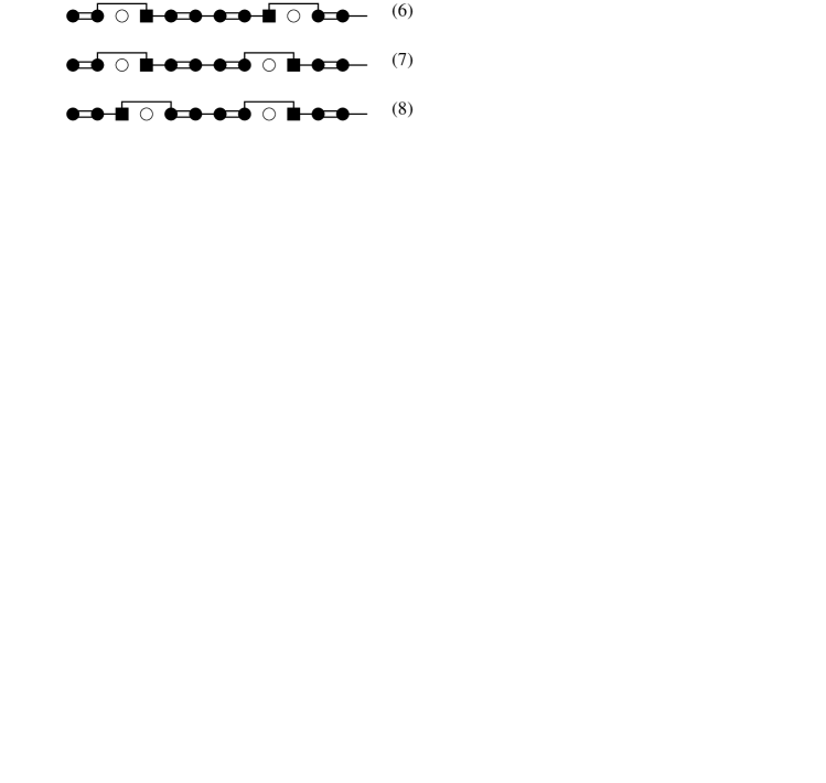
FIG. 6.: The eight inequivalent disorder realizations of the $12$ sites chain with $2$ impurities. The empty circles are the impurities, the filled symbols are the spin $1/2$ sites, the filled squares being the solitons. A double line stands for a strong bond ($J+\delta$) and a single line stands for a weak bond ($J-\delta$).

FIG. 7.: Staggered magnetic field as a funtion of temperature for the eight disorder realizations ($J_{\perp}=0.315$).

FIG. 8.: Susceptibility versus temperature ($J_{\perp}=0.315$).

FIG. 9.: Variations of the overlap with the antiferromagnetic state as a function of temperature ($J_{\perp}=0.315$).

REFERENCES

- [1] M. Hase et al., Phys. Rev. Lett. 70, 3651 (1993); J.P. Pouget et al., Phys. Rev. Lett. 72, 4037 (1994); K. Hirota et al., Phys. Rev. Lett. 73, 736 (1994).
- [2] J. Riera and A. Dobry, Phys. Rev. B 51, 16098 (1995); G. Castilla, S. Chakravarty, and V.J. Emery, Phys. Rev. Lett. 75, 1823 (1995).
- [3] J.-G. Lussier et al. J. Phys. Condens. Matter 7, L325 (1995).
- [4] M. Hase et al., Physica B 215, 164 (1995).
- [5] M. Hase et al., J. Phys. Soc. Jpn. 65, 1392 (1996).
- [6] Y. Sasago et al., unpublished (1996).
- [7] J.-P. Renard et al. Europhys. Lett. 30, 475 (1995).
- [8] L.P. Regnault et al. Europhys. Lett. 32, 579 (1995).
- [9] D. Khomskii, W. Geertsma, and M. Mostovoy, cond-mat/9609244.
- [10] The correlation between the position of the impurities and of the solitons has been revealed in neutron scattering experiments on weakly doped samples in the presence of a strong magnetic field able to excite solitons[11].
- [11] V. Kiryukin, B. Keimer, J.P. Hill, and A. Vigliante, Phys. Rev. Lett. 76, 4608 (1996).
- [12] The assumption that each impurity releases one soliton is in fact more appropriate to describe the effect of Zn or Ni doping. However, there are claims that also Si-doping can be effectively represented by a random distribution of domain walls (see T. Ng, cond-mat/9610016).
- [13] J. Zhang, S. Chakravarty, and A.R. Bishop, cond-mat/9702185
- [14] M. Fabrizio and R. Mélin, cond-mat/9701149.
- [15] J.E. Hirsh, Phys. Rev. B 22, 5339 (1980); ibid., 5355 (1980).
- [16] D. Fisher, Phys. Rev. B 50, 3799 (1994).
- [17] C. Dasgupta and S.K. Ma, Phys. Rev. B 22, 1305 (1980).
- [18] G.B. Martins, E. Dagotto and J.A. Riera, Phys. Rev. B 54, 16032 (1996).
- [19] T.P. Eggarter and R. Riedinger, Phys. Rev. B 18, 569 (1978).
- [20] A.A. Gogolin, and V.I. Mel’nikov, Sov. Phys. JETP 46, 369 (1977).
- [21] E. Lieb, T. Shultz and D. Mattis, Ann. Phys. 16, 407 (1961).
- [22] A.P. Young and H. Rieger, Phys. Rev. B 53, 8486 (1996).
- [23] N. Katoh and M. Imada, J. Phys. Soc. Jpn. 62, 3728 (1993).
- [24] S. Inagaki and H. Fukuyama, J. Phys. Soc. Jpn. 52, 3620 (1983).