Casimir forces in binary liquid mixtures

Abstract

If two ore more bodies are immersed in a critical fluid critical fluctuations of the order parameter generate long ranged forces between these bodies. Due to the underlying mechanism these forces are close analogues of the well known Casimir forces in electromagnetism. For the special case of a binary liquid mixture near its critical demixing transition confined to a simple parallel plate geometry it is shown that the corresponding critical Casimir forces can be of the same order of magnitude as the dispersion (van der Waals) forces between the plates. In wetting experiments or by direct measurements with an atomic force microscope the resulting modification of the usual dispersion forces in the critical regime should therefore be easily detectable. Analytical estimates for the Casimir amplitudes $\Delta$ in $d=4-\varepsilon$ are compared with corresponding Monte-Carlo results in $d=3$ and their quantitative effect on the thickness of critical wetting layers and on force measurements is discussed.

I Introduction

The phase diagram of a fluid is influenced by the presence of a surface in many different ways. Most prominent is the modification of the critical behavior of a fluid near a wall [1, 2] and the occurrence of new phase transitions induced by the wall such as wetting and drying [3]. For binary liquid mixtures external walls usually manifest themselves by a preferential affinity of the wall material for one of the components [4] which in the vicinity of the critical demixing point leads to the phenomenon of critical adsorption of the preferred component [5, 6]. If the system is made finite by the introduction of a second wall or by confining the system to another finite geometry the critical behavior of the fluid is modified again if the correlation length becomes comparable to the system size [7, 8, 9], where the size dependence of thermodynamic functions takes a scaling form. A finite geometry may also by generated spontaneously by a critical fluid if, e.g., a binary liquid mixture near its critical demixing transition forms a macroscopic wetting layer on the surface of a substrate [3, 10]. With the introduction of the second surface the variety of phenomena in the confined fluid goes far beyond critical finite-size scaling. Apart from the shift of the critical point of the system [11, 12] one encounters the phenomenon of capillary condensation [13] if the confining walls of the film geometry consist of the same material. The confinement of the fluid causes the liquid vapor coexistence line to be shifted away from the coexistence line of the bulk fluid into the one-phase regime of, e.g., the bulk vapor [12, 13]. For not too small wall separations a first order phase transition occurs from a confined vapor to a confined fluid as the undersaturation of the vapor is lowered at fixed temperature. In a constant-temperature plane of the phase diagram the line of two-phase coexistence is terminated by a capillary critical point characterized by a critical undersaturation and a critical wall separation beyond which capillary condensation no longer occurs [13]. Fluid layers growing on the inner walls of the capillary reduce its effective width and therefore generate correction terms to the well known Kelvin equation, which describes the aforementioned shift of the liquid vapor coexistence line as a function of the width of the capillary [14, 15].

From the theoretical point of view these phenomena can be described using density functional theory [13] and computer simulations of lattice gas models [12, 15]. These lattice gases are equivalent to Ising models, where the presence of the walls is described by surface fields which impose a finite surface magnetization on the Ising system. Density or concentration profiles of confined fluids or binary liquid mixtures, respectively, then translate to the magnetization profile of the Ising model. For the description of capillary condensation an Ising model with surface fields of the same sign is appropiate. The behavior of the system changes drastically, if opposing surface fields are considered. For a confined binary liquid mixture this means that the walls perfer different components. It turns out that in this case new quasi wetting transitions occur which can be first-order, critical, and tricritical and converge to the usual wetting transitions for growing wall separation [16]. Furthermore, two phase coexistence becomes restricted to temperatures located below the wetting temperature, if the surface fields are equal in opposite [17, 18]. The scaling behavior of the magnetization profile of an Ising model with opposing surface fields and the dependence of the interface position on the strength of the surface fields and the temperature has been studied thoroughly [19, 20]. Capillary condenstion does no longer occur, instead one observes the interface delocalization transition, i.e., the interface in the magnetization profile detaches from one of the walls and moves to the midplane of the film. This transition is second order and its critical point can be identified with the shifted critical point of the confined system, which in this case is located on the temperature axis [18]. Above the critical temperature the magnetization profiles become perfectly antisymmetric about the midplane of the film. By increasing the strength of the surface fields the critical temperature diminishes and in the limit of infinitely strong opposing surface fields the interface delocalization transition becomes suppressed at all.

Confined critical fluids also generate long-ranged forces between the confining walls [21], a phenomenon, which is a direct analogue of the well-known Casimir effect in electromagnetism [22]. Contrary to the usual dispersion forces, which are still under investigation for bodies with curved surfaces [23, 24, 25] and in presence of surface roughness [26, 27], critical Casimir forces are governed by universal scaling functions [9, 28]. At the bulk critical point these scaling functions reduce to the universal Casimir amplitudes [9, 28]. Especially for the strip geometry a variety of exact results are known from conformal invariance [29]. Away from the critical point the scaling functions are only known exactly for an Ising model confined to a strip in $d=2$ [30]. In higher dimensions only the spherical model has given access to further exact results for the scaling function of the Casimir force [31]. For the $O(N)$ universality class in $d=3$ so far only approximate results are known based on real space renormalitation [32], the field theoretic renormalization group [28], and Monte-Carlo simulations [33] for the film geometry. More recently Casimir forces between spherical particles immersed in a critical $O(N)$ symmetric systems have been investigated by field-theoretic methods augmented by conformal invariance considerations [34]. The field-theoretic treatment of critical systems confined to finite geometries is notoriously difficult, because the theory has to interpolate properly between critical behavior in different dimensions. There has been remarkable progress in devising alternative renormalization prescriptions beyond the standard minimal subtraction scheme [35] and in contructing effective actions for the Ising [36] and the more general $O(N)$ universality class [37]. However, these approaches have been devised for finite systems with symmetry conserving boundary conditions, their implementation for systems with symmetry breaking boundary conditions (surface fields), in which we are interested here, is still lacking. Within the framework of Ginzburg-Landau descriptions of critical finite systems in presence of surface fields the theoretical treatment has been limited to mean-field considerations for the film geometry [8, 11, 32, 38, 39] and concentric spheres [40] which can be mapped onto two-sphere and wall-sphere geometries at the bulk critical point by conformal transformations (see Ref. [34]). For tricritical systems between parallel plates a thorough mean-field analysis has also been performed [41]. In this paper we will concentrate on the Casimir forces in critical films in presence of surface fields, which is the adequate description for confined binary liquid mixtures [4].

The remainder of the presentation is planned as follows. In Sec. II we introduce the field-theoretic model of a confined binary liquid mixture close to its critical demixing point and an adequate Ising model for which the Monte-Carlo simulations of the Casimir force are performed. Sec. III is devoted to a survey of mean-field results for the scaling functions of the Casimir force. In Sec. IV we present one-loop results and Monte-Carlo estimates for the universal Casimir amplitudes which characterize the strength of the Casimir forces at bulk criticality. We restrict ourselves to the bulk critical point, because the one-loop calculations are based on the standard $\varepsilon$-expansion which cannot cope with the dimensional crossover. In Sec. V we discuss implications of the results presented in Sec. IV for force measurements and wetting experiments with critical binary liquid mixtures and we summarize the main results in Sec. VI. The one-loop calculation requires the knowledge of the mean-field order parameter profiles which are rederived and discussed in Appendix A. The eigenmode spectra are derived in Appendix B and the regularization of the one-loop mode sums is described in Appendix C.

II Model

For the analytical part of the current investigation the standard $\phi^{4}$ Ginzburg-Landau Hamiltonian ${\cal H}={\cal H}_{b}+{\cal H}_{s}$ for a $O(N)$ symmetric critical system in a parallel plate geometry is used. Specifically, the model is defined by the bulk Hamiltonian

$${\cal H}_{b}[{\bf\Phi}]=\int d^{d-1}x\int_{0}^{L}dz\left\{{1\over 2}(\nabla{\bf\Phi})^{2}+{\tau\over 2}{\bf\Phi}^{2}+{g\over 4!}({\bf\Phi}^{2})^{2}\right\},$$ (1)

where $L$ is the Film thickness, ${\bf\Phi}\equiv(\Phi_{1}({\bf x},z),\dots,\Phi_{N}({\bf x},z))$ is the $N$ component order parameter at the lateral position ${\bf x}$ and the perpendicular position $z$ $(0<z<L)$, $\tau$ is the bare reduced temperature, and $g$ is the bare coupling constant. The presence of the surfaces gives rise to the surface contribution

$${\cal H}_{s}[{\bf\Phi}]=\int d^{d-1}x\left\{{c_{1}\over 2}[{\bf\Phi}({\bf x},0)]^{2}+{c_{2}\over 2}[{\bf\Phi}({\bf x},L)]^{2}-{\bf h}_{1}\cdot{\bf\Phi}({\bf x},0)-{\bf h}_{2}\cdot{\bf\Phi}({\bf x},L),\right\}.$$ (2)

to the Ginzburg-Landau Hamiltonian, where $c_{1}$ and $c_{2}$ are the surface enhancements which characterize the surface universality class [2]. In mean field theory and within the dimensional regularization scheme for the field-theoretic renormalization group $c_{i}>0$ defines the ordinary $(O)$ surface universality class and $c_{i}<0$ defines the extraordinary $(E)$ surface universality class. The leading critical behavior of a semiinfinite system with an $O$ or an $E$ surface is described by the two stable renormalization group fixed point values $c=+\infty$ and $c=-\infty$, respectively. Finite positive or negative values of $c_{i}$ only yield corrections to the leading behavior. Within this setting $c=0$ is an unstable fixed point, so that $(\tau,c)=(0,0)$ has meaning of a multicritical point at which both the bulk and the surface of a semiinfinite system simultaneously undergo a second order phase transition [2]. This mulitcritical point defines a surface universality class in its own right which is commonly denoted as the surface-bulk $(SB)$ or special universality class. In the language of a spin model $c$ denotes the deviation of the exchange interaction between spins in the surface from its value at the multicritical point [see also Eq. (3) below].

The quantities ${\bf h}_{1}$ and ${\bf h}_{2}$ denote surface fields which explicitly break the $O(N)$ symmetry of the model. In case of a broken symmetry at the surface in principle also cubic surface fields need to be considered [5]. However, for the investigation of the leading critical behavior in the presence of nonzero linear surface fields cubic surface fields can be disregarded [5].

As pointed out in Sec. I a wall which is in contact with a binary liquid mixture will in general show some preferential affinity for one of the components so that the composition profile varies as a function of the perpendicular coordinate $z$. This situation can be represented by setting $c_{1}\geq 0$ and $c_{2}\geq 0$ in Eq. (2) and prescribing finite values for the surface fields ${\bf h}_{1}$ and ${\bf h}_{2}$. The phase transition in the bulk in presence of nonzero surface fields is called the normal transition [42]. As far as the leading critical behavior is concerned the normal transition is equivalent to the usual extraordinary transition [2, 42], which can be represented by setting ${\bf h}_{1}={\bf h}_{2}=0$ and choosing $c_{1}<0$ and $c_{2}<0$. In the following we will therefore exclusively use the surface field picture of the extraordinary transition.

In the field-theoretic analysis only the cases of strictly parallel and strictly antiparallel surface fields ${\bf h}_{i}=(h_{i},0,\dots,0)$, $i=1,2$ will be considered. For the leading critical behavior it is sufficient to discuss only the limiting cases $h_{1},h_{2}\to\pm\infty$ [2]. The above restriction to parallel and antiparallel surface fields then means that we only consider the two cases $h_{1}=h_{2}\to+\infty$ and $h_{1}=-h_{2}\to+\infty$. To simplify the notation we will refer to the former case as the $(+,+)$ boundary condition and to the latter case as the $(+,-)$ boundary condition which are the only combinations $(E,E)$ of the $E$ surface universality class in the film geometry considered here. One can also combine a symmetry breaking $E$ surface with a symmetry conserving $O$ or $SB$ surface. However, as will be demonstrated below, the combinations $(O,E)$ and $(SB,E)$ can be extracted from the analysis of the cases $(+,-)$ and $(+,+)$, respectively.

For the numerical part of this investigation we restrict ourselves to the case $N=1$ which is the most interesting one in view of applications of the results to binary liquid mixtures. The simulations are performed for a spin - $1\over 2$ Ising model confined to a film geometry in $d=3$ dimensions defined by the Hamiltonian

$${\cal H}_{I}=-J\sum_{<({\bf x},z),({\bf x^{\prime}},z^{\prime})>}s({\bf x},z)s({\bf x^{\prime}},z^{\prime})-H_{1}\sum_{\bf x}s({\bf x},1)-H_{2}\sum_{\bf x}s({\bf x},L),$$ (3)

where $J$ is the excange coupling constant, $<({\bf x},z),({\bf x^{\prime}},z^{\prime})>$ denotes a nearest neighbor pair of spins and the spins $s({\bf x},z)$ can take the values 1 and $-1$. The underlying lattice is supposed to be simple cubic with $L^{\prime}$ lattices sites and periodic boundary conditions in the $x$ and $y$ directions. In the $z$ direction the lattice has $L\ll L^{\prime}$ sites and the missing bonds in the two surface layers at $z=1$ and $z=L$ are left open. In order to simulate the model at the normal transition Eq. (3) contains two surface terms by which the spins in the two surface layers are coupled to surface fields $H_{1}$ and $H_{2}$, respectively. Infinite surface fields are simply realized by fixing all spins in the surface to a fixed value 1 or $-1$ depending on the sign of the surface field. In the model defined by Eq. (3) the surface exchange coupling constant $J_{1}$ has the fixed value $J_{1}=J$. It has been shown by Monte-Carlo simulations of spin - $1\over 2$ Ising models that the $SB$ multicritical point is characterized by the special value $J_{1c}\simeq 1.50J$ [43] of the surface coupling constant $J_{1}$. Apart from corrections to scaling the $O$ surface universality class is represented by the condition $J_{1}<J_{1c}$ [2] which is fulfilled by Eq. (3) due to $J_{1}=J<J_{1c}$. Therefore only the $O$ surface universality class ($H_{1}=0$ or $H_{2}=0$) and the $E$ surface universality class ($H_{1}\neq 0$ or $H_{2}\neq 0$) can be studied with the above Ising model Hamiltonian. The film geometry underlying Eq. (3) then allows the investigation of the four combinations $(O,O)$, $(O,E)$, $(+,+)$, and $(+,-)$ of boundary conditions by a Monte-Carlo simulation, where the combination $(O,E)$ means $(O,+)$ or, equivalently, $(O,-)$. The principal setup of a Monte-Carlo algorithm for a measurement of the Casimir force in lattice models is described in Ref. [33] to which the reader is referred for further details.

III Landau theory

The presence of a symmetry breaking surface field implies a nonvanishing order parameter profile for all $\tau$ (see Appendix A), which substantially complicates the field theoretic analysis of the Casimir effect as compared to the case of symmetry conserving boundary conditions discussed in Ref. [28]. On the other hand the leading (mean field) contribution to the Casimir amplitude can be determined without any detailed knowledge about the functional form of the order parameter profile. We briefly illustrate this for the case $\tau=0$ and $N=1$, i.e., ${\bf\Phi}=(\Phi,0,\dots,0)$ in Eqs. (1) and (2). In the mean field approximation the order parameter profile has the form $\overline{\bf\Phi}({\bf x},z)=(M(z),0,\dots,0)$, where $M(z)$ solves the Euler-Lagrange equations given by Eqs. (A1) and (A2). Inserting $\overline{\bf\Phi}$ into Eqs. (1) and (2) for $\tau=0$ and integrating by parts using Eqs. (A1), (A2), and (A4) ${\cal H}[\overline{\bf\Phi}]$ can be evaluated without solving the Euler-Lagrange equations for $M(z)$ explicitly. The result is the mean field free energy of the film at bulk criticality and is given by

$${\cal H}[\overline{\bf\Phi}] = {c_{1}\over 6}M^{2}(0)+{c_{2}\over 6}M^{2}(L)-{2\over 3}h_{1}M(0)-{2\over 3}h_{2}M(L)$$ (4)

$$+ {L\over 3}\left[{1\over 2}M^{\prime 2}(z_{0})-{g\over 4!}M^{4}(z_{0})\right],$$ (6)

where $h_{1}$ and $h_{2}$ denote the first component of ${\bf h}_{1}$ and ${\bf h}_{2}$, respectively, and $z_{0}$ is an arbitrary reference point $0\leq z_{0}\leq L$ between the two surfaces of the film. The terms in the first line of Eq. (4) constitute the surface contribution to the mean field free energy and the contribution in the second line of Eq. (4) is the finite size part, where the square bracket yields the Casimir force (see below). As a direct implication of Eq. (A4) one finds that the above expression for the Casimir force does not depend on the reference point $z_{0}$. Note that due to $\tau=0$ the bulk contribution to Eq. (4) vanishes identically. For $\tau\neq 0$ ${\cal H}[\overline{\bf\Phi}]$ cannot be expressed in the same closed form as given by Eq. (4) and we therefore resort to the $zz$-component $T_{\perp\perp}$ of the stress tensor $T_{kl}({\bf x},z)$ in order to find a more general expression for the Casimir force. The stress tensor $T_{kl}$ is given by [44]

$$T_{kl} = {\partial{\bf\Phi}\over\partial x_{k}}\cdot{\partial{\bf\Phi}\over\partial x_{l}}-\delta_{kl}\left[{1\over 2}(\nabla{\bf\Phi})^{2}+{\tau\over 2}{\bf\Phi}^{2}+{g\over 4!}({\bf\Phi}^{2})^{2}\right]$$ (7)

$$- \left[{d-2\over 4(d-1)}+{\cal O}(g^{3})\right]\left[{\partial^{2}\over\partial x_{k}\partial x_{l}}-\delta_{kl}\nabla^{2}\right]{\bf\Phi}^{2},$$ (9)

where $\tau$ and $g$ have the same meaning as in Eq. (1). The scaling dimension of $T_{kl}$ is given by the spatial dimension $d$. In a film geometry $\langle T_{kl}\rangle$ is diagonal due to the lateral translational invariance of the film. From the conservation property $\partial\langle T_{kl}\rangle/\partial x_{k}=0$ one then concludes that $\langle T_{kl}\rangle$ does not depend on position and therefore $\langle T_{\perp\perp}\rangle$ can be directly identified with the Casimir force per unit area. Note that the evaluation of $\langle T_{kl}\rangle$ according to Eq. (7) for $x_{k}=x_{l}=z$ and for $\tau=0$ within the mean field approximation $\overline{\bf\Phi}({\bf x},z)=(M(z),0,\dots,0)$ for the order parameter yields the square bracket in Eq. (4).

We now turn to the mean field analysis of the Casimir force as a function of the reduced temperature $\tau$, where we first restrict ourselves to the case $N=1$ (Ising universality class). In view of later applications of the results to binary liquid mixtures near the critical demixing transition this is the most relevant case. For the mean field analysis alone it would not be neccessary to determine the full order parameter profiles. However, in order to perform the fluctuation expansion (see Sec. IV and Appendix B) precise knowledge about the profiles on the mean field level is indispensable. Details of the calculation are summarized in Appendix A. In the course of the calculations for the order parameter profiles one obtains the corresponding expressions for the Casimir forces as byproducts which will be discussed in the following paragraph.

As in Appendix A we write the mean field contribution $\langle T_{\perp\perp}\rangle_{0}$ to the Casimir force in the form $\langle T_{\perp\perp}\rangle_{0}=(6/g)t_{\perp\perp}$ and we only consider $t_{\perp\perp}$ in the following for simplicity. From the general theory of critical finite size scaling [7, 9] we expect $t_{\perp\perp}$ to take the scaling form

$$t_{\perp\perp}=L^{-d}F(y)\ ,\ y=\tau L^{1/\nu},$$ (10)

where $d=4$ and $\nu=1/2$ within mean field theory. Note that right at the upper critical dimension $d=d_{c}=4$ the prefactor $6/g$ of the Casimir force generates logarithmic finite-size corrections due to the fact that the renormalized counterpart $u$ of the coupling constant $g$ vanishes according to $u(l)\sim 1/\ln l$ for $l\to\infty$ at the renormalization group fixed point [45]. However, logarithmic corrections to scaling in $d=4$ will be disregarded here so that from the point of view of mean field theory the above prefactor is treated as a constant.

For the case of $(+,+)$ boundary conditions the scaling function $F_{+,+}(y)$ can be read off from Eqs. (A15) and (A17). The result is

$$F_{+,+}(y)=-(2K)^{4}k^{2}(1-k^{2}) \quad,\quad y=(2K)^{2}(2k^{2}-1);$$ (11)

$$F_{+,+}(y)=(2K)^{4}k^{2} \quad,\quad y=-(2K)^{2}(k^{2}+1),$$ (12)

where $K\equiv K(k)$ is the complete elliptic integral of the first kind and $0\leq k<1$. The $y$ dependence of $F_{+,+}$ according to Eq. (11) is given in the parametric form $y=y(k)$, where $y(k)$ is a monotonic function of $k$ so that the inverse $k=k(y)$ exists and constitutes the $y$ dependence of $F_{+,+}$ in a unique way. As can be seen from Eq. (11) the parameterizations of $F_{+,+}$ and $y$ for $y\geq-\pi^{2}$ and $y\leq-\pi^{2}$ are different. The reason for this is purely technical in the sense that negative values for $k^{2}$ are avoided (see Appendix A for details). There is no singularity of $F_{+,+}(y)$ at the point $y=-\pi^{2}$ ($k=0$). In fact, $F_{+,+}(y)$ is analytic for all values of $y$, because the critical point of the film $(T_{c}(L),h_{c}(L))$ is located off the temperature axis at a finite critical bulk field $h=h_{c}(L)\sim L^{-\Delta/\nu}$, where $\Delta$ is the gap exponent [8, 11]. Within mean field theory one has $\Delta=3/2$ so that $\Delta/\nu=3$. For $(+,-)$ boundary conditions the corresponding result for the scaling function $F_{+,-}(y)$ can be read off from Eqs. (A24) and (A26). One finds

$$F_{+,-}(y)=(2K)^{4}(1-k^{2})^{2} \quad,\quad y=2(2K)^{2}(k^{2}+1);$$ (13)

$$F_{+,-}(y)=(2K)^{4} \quad,\quad y=-2(2K)^{2}(2k^{2}-1),$$ (14)

where a parameterization analogous to the one in Eq. (11) has been used. The scaling function $F_{+,-}(y)$ is also analytic for all values of y, although the critical point of the film in the case of opposing surface fields is located on the temperature axis and is associated with the interface delocalization transition [18]. However, due to the limit $h_{1}=-h_{2}\to\infty$ performed here this critical point has been formally shifted to $y_{c}=-\infty$ so that it is no longer visible as a singularity in $F_{+,-}(y)$. Corresponding results for $(SB,+)$ and $(O,+)$ boundary conditions can be constructed from Eqs. (11) and (13) using the simple transformation $L\to 2L$ (see Appendix A). One obtains

$$F_{SB,+}(y)=\textstyle{1\over 16}F_{+,+}(4y) \quad,\quad F_{O,+}(y)=\textstyle{1\over 16}F_{+,-}(4y).$$ (15)

The scaling functions obtained so far still contain a bulk contribution which corresponds to a bulk pressure given by $t_{\perp\perp,bulk}=-\tau m_{b}^{2}-m_{b}^{4}$. For $\tau\geq 0$ one has $t_{\perp\perp,bulk}=0$ $(m_{b}=0)$ and for $\tau<0$ one has $t_{\perp\perp,bulk}=\tau^{2}/4$ $(m_{b}=\sqrt{-\tau/2})$. The bulk contribution $F_{bulk}(y)$ to the scaling functions given by Eqs. (11), (13), and (15) then has the simple form $F_{bulk}(y)=\theta(-y)\ y^{2}/4$ which contains the usual mean field singularity of the bulk free energy at $\tau=0$. In order to express the finite-size contribution to the Casimir force $\langle T_{\perp\perp}\rangle_{0}$ in the scaling form we define the scaling functions

$$f_{a,b}(y)\equiv F_{a,b}(y)-F_{bulk}(y)$$ (16)

which are displayed in Fig. 1 for $(a,b)=(+,+)$ and $(+,-)$. Their shapes resemble those of the corresponding scaling functions for the Ising model confined to a strip in $d=2$ [30]. The asymptotic behavior of the scaling functions for $y\to\pm\infty$ is governed by an exponential decay according to

$$f_{+,+}(y\to\infty) \simeq -16y^{2}\exp(-\sqrt{y}),$$ (17)

$$f_{+,+}(y\to-\infty) \simeq -16y^{2}\exp(-\sqrt{-2y}),$$ (18)

$$f_{+,-}(y\to\infty) \simeq 16y^{2}\exp(-\sqrt{y}),$$ (19)

$$f_{+,-}(y\to-\infty) \simeq 16y^{2}\exp(-\sqrt{-y/2}).$$ (20)

The scaling functions take quite sizable values over a surprisingly broad range of the scaling argument $y$. This may serve as a first indication that the Casimir forces provide a strong modification of the usual dispersion forces in a parallel plate geometry at the extraordinary transition. However, in order to estimate the absolute strength of the Casimir forces in binary liquid mixtures close to their critical demixing transition a renormalization group analysis of $f_{+,+}(y)$ and $f_{+,-}(y)$ is required (see Sec. IV).

FIG. 1.: Scaling functions $f_{+,+}(y)$ (solid line) and $f_{+,-}(y)$ (dashed line) according to Eqs. (11), (13), and (16). The $y$ range influenced by the bulk critical point $y=0$ is very broad and the asymptotic decay for $y\to\pm\infty$ is dominated by an exponential [see Eq. (17)]. Note that $f_{+,+}(y)$ and $f_{+,-}(y)$ take their extreme values at $y\simeq 10$ and $y\simeq-25$, respectively.

If the order parameter has $N>1$ components, the case of parallel surface fields is already covered by the above analysis of the $(+,+)$ boundary conditions for $N=1$, because in this case the order parameter only has one nonzero component parallel to the surface fields. For antiparallel surface fields, however, this is not as obvious, because the order parameter has the additional freedom to rotate across the film by a position dependent angle $\varphi(z)$. We illustrate this for the case $N\geq 2$ with ${\bf h}_{1}=(h_{1},0,\dots,0)$ and ${\bf h}_{2}=h_{1}\ (\cos\alpha,\sin\alpha,0,\dots,0)$ in the limit $h_{1}\to\infty$ and for $\tau=0$. A similar situation has been been discussed in Ref. [39] for $\tau\neq 0$. If the order parameter profile is written in the form ${\bf M}(z)=\sqrt{12/g}\ m(z)\ (\cos\varphi(z),\sin\varphi(z),0,\dots,0)$ one finds the Euler-Lagrange equations [see Eq. (A3) and Ref. [39]]

$$\left[\varphi^{\prime}(z)m^{2}(z)\right]^{\prime} = 0,$$ (21)

$$m^{\prime\prime}(z) = \varphi^{\prime 2}(z)m(z)+2m^{3}(z).$$ (22)

As boundary conditions for $\varphi(z)$ we choose $\varphi(0)=0$ and $\varphi(L)=\alpha$, because the order parameter should be parallel to ${\bf h}_{1}$ and ${\bf h}_{2}$, respectively, at the surfaces. The amplitude function $m(z)$ is positive and its qualitative behavior resembles that of the profile $m_{+,+}(z)$ [see Eqs. (A16) and (A18)]. From Eq. (7) we then find for the Casimir force

$$\langle T_{\perp\perp}\rangle_{0}\equiv(6/g)\ t_{\perp\perp}=(6/g)\ \left[\varphi^{\prime 2}(L/2)m^{2}(L/2)-m^{4}(L/2)\right].$$ (23)

Note that Eq. (23) allows a sign change of the Casimir force as a function of the angle $\alpha$ enclosed by the surface fields. Following Appendix A [see Eqs. (A4) and (A5)] the first integral of Eq. (21) is given by

$$\varphi^{\prime}(z) = c/m^{2}(z),$$ (24)

$$m^{\prime 2}(z) = -c^{2}/m^{2}(z)+m^{4}(z)+t_{\perp\perp},$$ (25)

where

$$t_{\perp\perp}=c^{2}/m^{2}(L/2)-m^{4}(L/2)$$ (26)

and $c$ is a constant such that

$$\alpha=\varphi(L)\quad\mbox{for}\quad\varphi(z)=c\int_{0}^{z}dz^{\prime}/m^{2}(z^{\prime}).$$ (27)

Just as for Eq. (A6) we apply the substitution $P(z)\equiv m^{2}(z)$ and eliminate $c$ using Eq. (26). All the information needed to calculate the Casimir force, i.e., $t_{\perp\perp}$ as a function of $\alpha$ is now contained in Eq. (27) and

$$P^{\prime 2}(z)=4\left[P^{3}(z)-P^{3}(L/2)+t_{\perp\perp}\left(P(z)-P(L/2)\right)\right]$$ (28)

which shows that $P(z)\equiv\wp(z;g_{2},g_{3})$ is a Weierstrass elliptic function, where the invariants $g_{2}$ and $g_{3}$ can be read off from Eq. (28). As we are focussing on the limit of infinite surface fields the film thickness $L$ is one of the basic periods of $P(z)$ [see Eqs. (A14) and (A23)], and therefore $P(z)$ has double poles at $z=0$ and $z=L$. Using Eq. (28) we can rewrite Eq. (27) and find a representation for $P(L/2)$ by performing a separation of variables in Eq. (28). Writing $t_{\perp\perp}$ in the scaling form [see Eq. (10)]

$$t_{\perp\perp}=L^{-4}g(\alpha)$$ (29)

and using the abbreviation $p\equiv L\sqrt{P(L/2)}$ one finds

$$p = \int_{1}^{\infty}\left[x^{3}-1+(x-1)p^{-4}g(\alpha)\right]^{-1/2}dx,$$ (30)

$$\alpha = \sqrt{1+p^{-4}g(\alpha)}\int_{1}^{\infty}x^{-1}\left[x^{3}-1+(x-1)p^{-4}g(\alpha)\right]^{-1/2}dx.$$ (32)

The solution of Eq. (30) is shown in Fig. 2. The Casimir force (i.e., $g(\alpha)$) grows monotonically from $\alpha=0$ to $\alpha=\pi$ at fixed $L$ and vanishes for the angle $\alpha=\pi/3$ which can also be derived directly from Eq. (30) by setting $g(\alpha)=0$. Furthermore it should be noted that according to Eqs. (11) and (16) one has $g(0)=F_{+,+}(0)=f_{+,+}(0)$ and according to Eqs. (13) and (16) one also has $g(\pi)=F_{+,-}(0)=f_{+,-}(0)$. The function $g(\alpha)$ therefore smoothly interpolates between $(+,+)$ and $(+,-)$ boundary conditions giving the same result for the Casimir force as the Ising universality class $(N=1)$ in these two cases.

FIG. 2.: Amplitude function $g(\alpha)$ of the Casimir force according to Eqs. (29) and (30). $g(\alpha)$ smoothly interpolates between $g(0)=f_{+,+}(0)$ and $g(\pi)=f_{+,-}(0)$ (see main text). The amplitude vanishes at $\alpha=\pi/3$.

We close this section with a short discussion of the analytic solution of Eqs. (28) and (30). Following the derivation described in Appendix A and using Eq. (27) the profile $m(z)=\sqrt{P(z)}$, the amplitude function $g(\alpha)$, and the angle $\alpha$ can be parameterized in terms of the modulus $k$ of the Jacobian elliptic functions. One finds

$$m(z) = {2K\over L}\left[{\mbox{dn}^{2}(\zeta;k)\over\mbox{sn}^{2}(\zeta;k)}+{2k^{2}-1\over 3}\right]^{1/2},$$ (33)

$$g(\alpha) = -{1\over 4}(2K)^{4}\left[1+{(2k^{2}-1)^{2}\over 3}\right],$$ (35)

$$\alpha = 2\left[{(1-2k^{2})(2-k^{2})\over 3(1+k^{2})}\right]^{1/2}\left[\Pi(1/3+k^{2}/3,k)-K\right]$$ (37)

and

$$m(z) = {2K\over L}\left[{\mbox{cn}^{2}(\zeta;k)\over\mbox{sn}^{2}(\zeta;k)\mbox{dn}^{2}(\zeta;k)}-{2(2k^{2}-1)\over 3}\right]^{1/2},$$ (38)

$$g(\alpha) = (2K)^{4}\left[1-{4(2k^{2}-1)^{2}\over 3}\right],$$ (40)

$$\alpha = \sqrt{6(1-2k^{2})}\left\{\left[{b\over 1-2k^{2}}+{2\over 3}\right]\left[\Pi(a,k)-K\right]\right.$$ (42)

$$- \left.\left[{a\over 1-2k^{2}}+{2\over 3}\right]\left[\Pi(b,k)-K\right]\right\},$$ (44)

where $\zeta=(2K/L)z$, $0\leq k^{2}\leq 1/2$, and the parameters $a$ and $b$ are given by

$$a = \textstyle{1\over 6}\left[1+4k^{2}+\sqrt{9-8(2k^{2}-1)^{2}}\right],$$ (45)

$$b = \textstyle{1\over 6}\left[1+4k^{2}-\sqrt{9-8(2k^{2}-1)^{2}}\right].$$ (46)

Furthermore $K\equiv K(k)$ and $\Pi(x,k)$ for $x=a,b$ denote the complete elliptic integrals of the first and the third kind, respectively. The angle $\alpha$ traverses the interval $[0,\pi]$ by decreasing $k^{2}$ from $k^{2}=1/2$ to $k^{2}=0$ in Eq. (33), changing to Eqs. (38) and (45) at $k^{2}=0$ and increasing $k^{2}$ back to $k^{2}=1/2$. The special point $k^{2}=0$ has no particular physical significance, it only marks a singular point in the above parametric representation of $g(\alpha)$. From Eq. (38) we identify $k^{2}=(2-\sqrt{3})/4$ as the parameter value, where $g(\alpha)=0$ or, equivalently, $\alpha=\pi/3$.

FIG. 3.: Amplitude $m(z)$ (solid line) and phase $\varphi(z)$ (dashed line) of a two component order parameter for surface fields at an angle of $\alpha=0.98\pi$ [$k^{2}\simeq 0.499$, see Eqs. (27) and (38) and main text]. $m(z)$ has been normalized to $m(L/10)$ so that $m(z)$ and $\varphi(z)$ can be plotted on the same scale.

Setting $k^{2}=1/2$ in Eq. (33) yields $m(z)=m_{+,+}(z)$ [see Eq. (A16) for $\tau=0$], $g(\alpha=0)=f_{+,+}(y=0)$ [see Eqs. (11) and (16)], and $\varphi(z)=0$ [see Eq. (27)]. This means that the order parameter profile is given by ${\bf M}(z)=\sqrt{12/g}\ (m_{+,+}(z),0,\dots,0)$ as anticipated from the case $N=1$ for $(+,+)$ boundary conditions. In the limit $k^{2}\to 1/2$ Eqs. (38) and (45) yield $m(z)=|m_{+,-}(z)|$ [see Eq. (A25) for $\tau=0$], $g(\alpha=\pi)=f_{+,-}(y=0)$ [see Eqs. (13) and (16)], whereas $\varphi(z)$ here is given by the step function $\varphi(z)=\pi\ \theta(z/L-1/2)$. The order parameter profile is then given by ${\bf M}(z)=\sqrt{12/g}(m_{+,-}(z),0,\dots,0)$ which shows that also for antiparallel surface fields mean field theory for an $N$-component order parameter is already captured by the case $N=1$. We illustrate this remarkable behavior of ${\bf M}(z)$ for $\alpha/\pi=0.98$, i.e., a situation close to antiparallel surface fields. The corresponding modulus $k$ [see Eqs. (38) and (45)] is given by $k^{2}\simeq 0.499$. The phase $\varphi(z)$ and the amplitude $m(z)$ of the order parameter are shown in Fig. 3. The order parameter rotates by almost the full amount $\alpha$ in a narrow interval around $z=L/2$, where $m(z)$ is smallest. In the limit $\alpha\to\pi$ this interval shrinks to the point $z=L/2$, where $m(z)$ vanishes and $\varphi(z)$ becomes discontinuous.

Although the Casimir force is governed by universal scaling functions [28, 9] it is not possible to estimate their absolute magnitude within Landau (mean field) theory. The reason is that for the boundary conditions considered here these scaling functions contain a common prefactor which depends on the bare coupling constant $g$ and therefore has a value inaccessible by pure mean field arguments. In order to at least partly fill this gap we now turn to the field theoretic analysis of the Casimir force at bulk criticality.

IV Casimir amplitudes

At the bulk critical temperature $T=T_{c}$ $(\tau=0)$ the Casimir forces in a film are governed by the universal Casimir amplitudes $\Delta_{a,b}$ which explicitly depend on the two surface universality classes combined in the film. For $N>1$ order parameter components the Casimir amplitudes may also depend on continuously varying parameters, as demonstrated above for the case $N=2$ with tilted surface fields. For $T\neq T_{c}$ $(\tau\neq 0)$ these amplitudes have to be replaced by universal scaling functions $\theta_{a,b}(y)$ of a suitably chosen scaling argument $y$ [28], which will not be considered in this section.

The Casimir amplitude is defined as the finite-size amplitude of the free energy of a film at bulk criticality [9, 28]. Translating this definition to the force one finds

$$-{\partial\over\partial L}f(T_{c},L)=\langle T_{\perp\perp}\rangle=(d-1)\Delta_{a,b}L^{-d}$$ (47)

in $d$ dimensions and for $\tau=0$, where $f(T_{c},L)\equiv{\cal F}(T=T_{c},L)/(A\ k_{B}T_{c})$ is the critical part of the free energy per unit area $A$ of the plates. Following Ref. [28] $k_{B}T_{c}$ is used as the natural energy unit for the free energy, where $k_{B}$ is the Boltzmann constant. As a first step beyond Landau theory the contribution of Gaussian fluctuations to the Casimir force, i.e., to the amplitudes $\Delta_{a,b}$ will be investigated here. We introduce the fluctuation part $\widetilde{\bf\Phi}$ of the order parameter ${\bf\Phi}$ by ${\bf\Phi}=\overline{\bf\Phi}+\widetilde{\bf\Phi}$, where $\overline{\bf\Phi}\equiv{\bf M}(z)=\sqrt{12/g}\ (m(z),0,\dots,0)$ is the mean field order parameter profile discussed in the preceding section and Appendix A. Inserting the above decomposition of ${\bf\Phi}$ into Eqs. (1) and (2) for $\tau=0$ and $c_{1}=c_{2}=0$ and keeping only the quadratic terms in $\widetilde{\bf\Phi}=(\widetilde{\phi}_{1},\dots,\widetilde{\phi}_{N})$ we obtain

$${\cal H}[{\bf\Phi}] = {\cal H}[\overline{\bf\Phi}]+{1\over 2}\int d^{d-1}x\int_{0}^{L}dz\left\{(\nabla\widetilde{\bf\Phi})^{2}+\left[6m^{2}(z)\widetilde{\phi}_{1}^{2}+2m^{2}(z)\left(\widetilde{\phi}_{2}^{2}+\dots+\widetilde{\phi}_{N}^{2}\right)\right]\right\}$$ (49)

$$+{\cal O}\left[\widetilde{\phi}_{1}\widetilde{\bf\Phi}^{2}\right]+{\cal O}\left[(\widetilde{\bf\Phi}^{2})^{2}\right],$$

where ${\bf h}_{1}=\pm{\bf h}_{2}=(h_{1},0,\dots,0)$ in the limit $h_{1}\to\infty$ is implicitly assumed. The mean field contribution ${\cal H}[\overline{\bf\Phi}]$ to Eq. (49) has already been discussed in Eq. (4). Following Eq. (49) we decompose the Casimir force into the mean field part, a Gaussian part, and higher order corrections according to

$$\langle T_{\perp\perp}\rangle=\langle T_{\perp\perp}\rangle_{0}+\langle T_{\perp\perp}\rangle_{1}+{\cal O}(g)=(6/g)t_{\perp\perp}+\langle T_{\perp\perp}\rangle_{1}+{\cal O}(g).$$ (50)

In order to determine $\langle T_{\perp\perp}\rangle_{1}$ from Eq. (7) one also needs the cubic terms in Eq. (49) and we will therefore not follow this approach any further. It is much more convenient to determine $\langle T_{\perp\perp}\rangle_{1}$ from the Gaussian contribution to the free energy by taking its first derivative with respect to the film thickness $L$ [28]. Following Ref. [28] this can be done most easily in a spectral representation of the Gaussian Hamiltonian given by Eq. (49). For the evaluation of $\langle T_{\perp\perp}\rangle_{1}$ only the eigenvalue spectrum is needed. According to Eq. (49) the spectrum consists of a longitudinal part $\epsilon_{n}^{(2)}$ characterizing the eigenmodes of the longitudinal fluctuations $\widetilde{\phi}_{1}$ of the order parameter and a transverse part $\epsilon_{n}^{(1)}$ which is the same for each of the $N-1$ transverse components $(\widetilde{\phi}_{2},\dots,\widetilde{\phi}_{N})$ of the order parameter fluctuations. The spectra $\epsilon_{n}^{(1)}$ and $\epsilon_{n}^{(2)}$ are determined in Appendix B. Once the eigenvalues are given one can employ the dimensional regularization scheme and according to Ref. [28] we find

$$f(T_{c},L)={\cal H}[\overline{\bf\Phi}]+{\Gamma\left[(3-d)/2\right]\over 2^{d-1}\pi^{(d-1)/2}(d-1)}\left[\sum_{n=3}^{\infty}\left(\epsilon_{n}^{(2)}\right)^{(d-1)/2}+(N-1)\sum_{n=2}^{\infty}\left(\epsilon_{n}^{(1)}\right)^{(d-1)/2}\right]$$ (51)

for the critical part free energy within the Gaussian approximation in $d$ dimensions. The $L$ dependence of the Gaussian contribution to $f(T_{c},L)$ is completely determined by the $L$ dependence of the eigenvalues. From simple dimensional analysis one has $\epsilon_{n}^{(i)}\sim L^{-2}$ so that $d\epsilon_{n}^{(i)}/dL=-(2/L)\epsilon_{n}^{(i)}$ for $i=1,2$. From Eqs. (47) and (51) we find

$$\langle T_{\perp\perp}\rangle={6\over g}t_{\perp\perp}+{\Gamma\left[(3-d)/2\right]\over 2^{d-1}\pi^{(d-1)/2}L}\left[\sum_{n=3}^{\infty}\left(\epsilon_{n}^{(2)}\right)^{(d-1)/2}+(N-1)\sum_{n=2}^{\infty}\left(\epsilon_{n}^{(1)}\right)^{(d-1)/2}\right]+{\cal O}(g)$$ (52)

for the Casimir force in the Gaussian approximation. The mode sums in Eq. (52) diverge for $d=4-\varepsilon$ and we therefore employ the dimensional regularization scheme. Furthermore, the above sums yield an UV singularity in the typical form $1/\varepsilon$ which must be treated analytically in order to facilitate the renomalization of Eq. (52). Both objectives can be achieved with the asymptotic expansions of the eigenvalues $\epsilon_{n}^{(1)}$ and $\epsilon_{n}^{(2)}$ for large mode numbers $n$ which are given by Eqs. (B14) and (B18). The regularization of the mode sums and the analytical treatment of the $1/\varepsilon$ pole is summarized in Appendix C. Using the results from Appendix B and C we now investigate the different boundary conditions separately, where the mean-field results given by Eqs. (11), (13), and (15) are only needed for $k^{2}=1/2$ $(\tau=0)$.

For the renormalization of the Casimir force given by Eq. (52) we use the conventions of Ref. [28] and define the renormalized coupling constant $u$ by

$$g=2^{d}\pi^{d/2}\mu^{4-d}Z_{u}u\quad,\quad Z_{u}=1+{N+8\over 3}{u\over\varepsilon}+{\cal O}(u^{2}),$$ (53)

where $\mu$ is an arbitrary momentum scale and $d=4-\varepsilon$ in the following. The infrared stable fixed point value $u^{*}(\varepsilon)$ of the renormalized coupling constant $u$ is given by [2]

$$u^{*}(\varepsilon)={3\over N+8}\varepsilon+{9(3N+14)\over(N+8)^{3}}\varepsilon^{2}+{\cal O}(\varepsilon^{3}).$$ (54)

For later reference we also quote the 3-loop estimate [46]

$$u_{1}^{*}(\varepsilon)={\varepsilon\over 3}+{17\over 81}\varepsilon^{2}+\left({709\over 17496}-{4\over 27}\ \zeta(3)\right)\varepsilon^{3}+{\cal O}(\varepsilon^{4})$$ (55)

of the fixed point value $u^{*}$ for $N=1$, where $\zeta(3)\simeq 1.20206$ is a special value of the Riemann zeta function. In order to improve the predictive quality of a low-order $\varepsilon$-expansion for $\varepsilon=1$ $(d=3)$ in a simple way one may try to include exact results for the quantity in question in $d=2$ in the sprit of a Padé approximant in the variable $\varepsilon$. This can be applied rather successfully to the Casimir amplitude $\Delta_{per}$ thus improving the agreement between the field-theoretic prediction [28] and the Monte-Carlo estimate [33] in $d=3$. We will therefore follow the same procedure here, where the case of $(SB,+)$ boundary conditions must be excluded, because the $SB$ multicritical point does not exist in $d=2$.

The renormalized expression for $\langle T_{\perp\perp}\rangle$ for $(+,+)$ boundary conditions can be obtained by inserting the mean field result given by Eq. (11) for $y=0$ and the regularized mode sum given by Eq. (C11) into Eq. (52) and by applying the renormalization prescription given by Eq. (53). After expanding all $d$ dependent quantities to first order in $\varepsilon$ [see Eq. (C30)] the $1/\varepsilon$ pole coming from Eq. (C11) is cancelled, i.e., the UV singularity has been consistently removed from the theory. The Casimir force then follows by evaluating the resulting renormalized expression for $\langle T_{\perp\perp}\rangle$ at the renormalization group fixed point $u=u^{*}(\varepsilon)$ given by Eq. (54). The $\varepsilon$-expansion of the universal Casimir amplitude $\Delta_{+,+}$, which characterizes the strength of the Casimir force in a critical film with parallel surface fields, is finally obtained by applying the definition of $\Delta_{a,b}$ given by Eq. (47). The algebraic manipulations involved here starting from Eqs. (52), (C11), and (53) are absolutely elementary, so that we only quote the final result

$$\Delta_{+,+}=-{\pi^{d/2}\Gamma(d/2)\over 2u^{*}(\varepsilon)}\left({K\over\pi}\right)^{4}\left[1-{9\varepsilon\over N+8}\ 0.6853+\varepsilon\ {N-1\over N+8}\ 0.1242+{\cal O}(\varepsilon^{2})\right],$$ (56)

where part of the $\varepsilon$-expansion has been resummed consistently to first order in $\varepsilon$ using Eq. (C31). For $(+,-)$ boundary conditions the same procedure can be applied using Eq. (13) for $y=0$ and Eqs. (52) and (C14). One finds

$$\Delta_{+,-}=2{\pi^{d/2}\Gamma(d/2)\over u^{*}(\varepsilon)}\left({K\over\pi}\right)^{4}\left[1-{9\varepsilon\over N+8}\ 0.2822+\varepsilon\ {N-1\over N+8}\ 0.4066+{\cal O}(\varepsilon^{2})\right].$$ (57)

From Eq. (15) for $y=0$ and Eqs. (52) and (C21) one has for $(SB,+)$ boundary conditions

$$\Delta_{SB,+}=-{\pi^{d/2}\Gamma(d/2)\over 32u^{*}(\varepsilon)}\left({K\over\pi}\right)^{4}\left[1+{9\varepsilon\over N+8}\ 1.7141+\varepsilon\ {N-1\over N+8}\ 2.8448+{\cal O}(\varepsilon^{2})\right].$$ (58)

From Eq. (15) for $y=0$ and Eqs. (52) and (C27) one finally has for $(O,+)$ boundary conditions

$$\Delta_{O,+}={\pi^{d/2}\Gamma(d/2)\over 8u^{*}(\varepsilon)}\left({K\over\pi}\right)^{4}\left[1+{9\varepsilon\over N+8}\ 0.1988+\varepsilon\ {N-1\over N+8}\ 0.2289+{\cal O}(\varepsilon^{2})\right].$$ (59)

Note that $u^{*}(\varepsilon)$ in the above expressions is given by Eq. (54). It is remarkable that the coefficients of the Gaussian contribution to $\Delta_{SB,+}$ given by Eq. (58) are much bigger than the corresponding coefficients in Eqs. (56), (57), and (59). This may be due to the fact that the order parameter near a $SB$ surface is much more susceptible to fluctuations than near $O$ or $E$ surfaces.

In the Ising universality class $(N=1)$ in $d=2$ three of the above Casimir amplitudes are known exactly from conformal field theory [29]. They are given by

$$\Delta_{+,+}=-{\pi\over 48}\quad,\quad\Delta_{+,-}={23\over 48}\pi\quad,\quad\Delta_{O,+}={\pi\over 24}.$$ (60)

The construction of a Padé approximant from Eqs. (56), (57), and (59) for $N=1$ which extrapolates to the amplitudes given by Eq. (60) for $\varepsilon=2$ is arbitrary to a certain degree. If one uses Eq. (55) instead of Eq. (54) for $N=1$ and introduces an additional $\varepsilon^{2}$-contribution to the square bracket of Eqs. (56), (57), and (59) such that Eq. (60) is reproduced for $\varepsilon=2$ one finds the interpolation formulas

$$\Delta_{+,+} = -{\pi^{d/2}\Gamma(d/2)\over 2u_{1}^{*}(\varepsilon)}\left({K\over\pi}\right)^{4}\left[1-0.6853\ \varepsilon+0.1275\ \varepsilon^{2}\right],$$ (61)

$$\Delta_{+,-} = 2{\pi^{d/2}\Gamma(d/2)\over u_{1}^{*}(\varepsilon)}\left({K\over\pi}\right)^{4}\left[1-0.2822\ \varepsilon+0.0914\ \varepsilon^{2}\right],$$ (63)

$$\Delta_{O,+} = {\pi^{d/2}\Gamma(d/2)\over 8u_{1}^{*}(\varepsilon)}\left({K\over\pi}\right)^{4}\left[1+0.1988\ \varepsilon-0.0707\ \varepsilon^{2}\right].$$ (65)

Numerical estimates of the Casimir amplitudes in $d=3$ obtained from the above analytical formulas are summarized in Table I.

Table I. Casimir amplitudes for the Ising universality class in $d=3$. The values labelled by $\varepsilon=1$ are obtained by evaluating Eqs. (68), (56), (57), (58), and (59) for $N=1$ and $\varepsilon=1$. The values labelled $d=3$ are obtained from Eqs. (69) and (61) for $d=3$ $(\varepsilon=1)$. The Monte-Carlo estimates obtained from the serial version of the algorithm presented in Ref. [33] are labelled by ’MC’ (see also main text). Statistical errors (one standard deviation) are in the last two digits as indicated inside the parenthesis. The last line shows Migdal-Kadanoff estimates taken from Ref. [32].

	$\ \ \Delta_{per}$	$\ \ \Delta_{O,O}$	$\ \ \Delta_{+,+}$	$\ \Delta_{+,-}$	$\ \Delta_{SB,+}$	$\ \Delta_{O,+}$
$\varepsilon=1$	$-0.1116$	$-0.0139$	$-0.173$	$1.58$	$-0.093\ \ \$	$0.165$
$d=3$	$-0.1315$	$-0.0164$	$-0.326$	$2.39$		$0.208$
MC	$-0.1526(10)\$	$-0.0114(20)\$	$-0.345(16)\$	$2.450(32)\$		$0.1873(70)\$
Ref.[32]		$-0.015$	$\ \ 0$	$0.279$	$\ \ \ 0.017$	$0.051$

In $d=3$ and for $N=1$ the Casimir amplitudes $\Delta_{O,O}$, $\Delta_{O,+}$, $\Delta_{+,+}$, and $\Delta_{+,-}$ can be measured by a Monte-Carlo simulation of the Ising model defined by Eq. (3). The algorithm and its special adaptation to the measurement of the Casimir amplitude is presented in Ref. [33] in detail. We therefore only briefly describe the differences between the implementations used here and in Ref. [33]. The present implementation of the algorithm utilizes a serial hybrid update scheme which consists of a Metropolis update sweep of the whole lattice followed by a Wolff update. The length of the equilibration and the measurement period used here correspond to those in Ref. [33]. The slab geometry contains $L^{\prime 2}\times L$ lattice sites, where $L^{\prime}/L$ must be chosen as large as possible in order to approximate the infinite slab geometry. In practice already $L^{\prime}=4L$ turns out to be sufficient, i.e., the results obtained for this choice agree with those for $L^{\prime}=6L$ within a fraction of one standard deviation. The thickness $L$ of the slab has been varied between $L=12$ and $L=32$ layers. As in Ref. [33] we use the multiple histogram technique [47], where the number of histograms taken has been increased from 25 to 31 for $L>24$ on order to guarantee sufficient overlap between adjacent histograms [33]. The simulations were run on DEC Alpha workstations at the University of Wuppertal and the total amount of CPU time used is equvalent to about one year of CPU time on a DEC 3000 workstation.

The serial implementation of the algorithm has been tested for the Casimir amplitude $\Delta_{per}$ with $L^{\prime}=4L$ and $L^{\prime}=6L$ for $L=20$ and $L=24$. The estimates for $\Delta_{per}$ obtained with these four lattice sizes agree within their statistical error and give the final estimate

$$\Delta_{per}=-0.1526\pm 0.0010,$$ (66)

which is in perfect greement with the estimate obtained from the parallel algorithm [33]. The amplitude $\Delta_{O,O}$ has been measured for the same lattices sizes and for $\Delta_{O,+}$ additional simulations were performed with $L=28$ and $L^{\prime}=4L$. All individual measurements agree within their statistical error and the final estimates are shown in Table I. For $(+,+)$ and $(+,-)$ boundary conditions, however, the situation is different. For $\Delta_{+,+}$ measurements have been made for $12\leq L\leq 32$ and $L^{\prime}=4L$, the individual estimates are displayed in Fig.4 as a function of $L$.

FIG. 4.: Monte-Carlo estimates of the Casimir amplitude $\Delta_{+,+}$ as a function of the number of layers $L$ in a $L^{\prime 2}\times L$ slab for $L^{\prime}=4L$. The size of the error bars represents one standard deviation. The data point at $L=32$ is taken as the final estimate (see Table I).

The estimates show a clear systematic dependence on $L$ and apparently even for $L=32$ layers the asymptotic regime has not yet been reached. The last three data points fall onto a straight line within their error bars so that the data cannot be extrapolated to an asymptotic value. As the current Monte-Carlo estimate for $\Delta_{+,+}$ we therefore take the measurement for the biggest system ($L=32$, $L^{\prime}=4L$) (see Table I). The situation for $\Delta_{+,-}$ is similar. The individual measurements are shown in Fig. 5 for $12\leq L\leq 28$ $(L^{\prime}=4L)$. Again, the asymptotic regime has not been reached for the biggest system, but this time it is possible to estimate the asymptotic value for $\Delta_{+,-}$ by a least square fit of the function

$$\Delta_{+,-}^{eff}(L)=\Delta_{+,-}+D\exp(-\kappa L)$$ (67)

to the data for $L\geq 16$ using $\Delta_{+,-}$, $D$, and $\kappa$ as fit parameters.

FIG. 5.: Monte-Carlo estimates of the Casimir amplitude $\Delta_{+,-}$ as a function of the number of layers $L$ in a $L^{\prime 2}\times L$ slab for $L^{\prime}=4L$. The size of the error bars represents one standard deviation. The dashed line shows a fit of Eq. (67) to the data for $L\geq 16$ giving the estimate of $\Delta_{+,-}$ displayed in Table I. The absolute size of the errorbars is about twice that in Fig. 4.

The exponential $L$ dependence of $\Delta_{+,-}^{eff}(L)$ in Eq. (67) is motivated by the short-ranged nature of the interaction in Eq. (3). The error of the amplitude $\Delta_{+,-}$ is estimated by taking the maximal error of the individual measurements involved in the fit. All estimates obtained from Eqs. (56), (57), and (59) for $N=1$, from Eq. (61), and our Monte-Carlo estimates are summarized in Table I. For completeness we also display estimates for $\Delta_{per}$ and $\Delta_{O,O}$ obtained from the partially resummed $\varepsilon$-expansions [21]

$$\Delta_{per}=-N{\Gamma(d/2)\zeta(d)\over\pi^{d/2}}\left(1-{5\over 4}{N+2\over N+8}\ \varepsilon+{\cal O}(\varepsilon^{2})\right)\quad,\quad\Delta_{O,O}=2^{-d}\Delta_{per}$$ (68)

for $N=1$ and from the Padé approximants [21, 33]

$$\Delta_{per}=-{\Gamma(d/2)\zeta(d)\over\pi^{d/2}}\left(1-{5\over 4}{4-d\over 7-d}\right)\quad,\quad\Delta_{O,O}=2^{-d}\Delta_{per},$$ (69)

which reproduce the exact results [29]

$$\Delta_{per}=-{\pi\over 12}\quad,\quad\Delta_{O,O}=-{\pi\over 48}$$ (70)

in $d=2$. For comparison we also reproduce Migdal-Kadanoff estimates for the Casimir amplitudes in $d=3$ from Ref. [32]. The agreement between the Padé approximants and the Monte-Carlo estimates is quite satisfactory, except for $\Delta_{O,O}$ which seems to be closer to the partially resummed $\varepsilon$-expansion and the Migdal-Kadanoff estimate. However, the amplitude is rather small and therefore the relative statistical error of the Monte-Carlo estimate, which is one standard deviation, is very large (20%, see Table I). In view of Fig. 4 the Monte-Carlo estimate for $\Delta_{+,+}$ given in Table I constitutes only an upper bound for the true amplitude and must therefore also be handled with caution. The fit procedure used to extract $\Delta_{+,-}$ from the data shown in Fig. 5 is also susceptible to systematic errors to a certain extent. However, compared to the parameters $D$ and $\kappa$ in Eq. (67) the resulting estimate for $\Delta_{+,-}$ is quite robust with respect to, e.g., changes in the number of data points included in the fit. The obtained variation of $\Delta_{+,-}$ is in the same order of magnitude as the statistical error given in Table I. With regard to their reliability the analytical and the Monte-Carlo estimates of $\Delta_{+,+}$, $\Delta_{+,-}$, and $\Delta_{O,+}$ seem to be a substantial improvement over the Migdal-Kadanoff results.

V Experimental implications

A typical experimental setting, within which the film geometry considered here is of particular interest, is provided by wetting experiments performed on plane and chemically homogeneous substrates [3, 10, 48]. The equilibrium thickness $L$ of the wetting layer is determined by the minimum of the effective interface potential [3]. It is given by the grand canonical free energy of a liquid layer of a prescribed thickness $l$, which is in contact with the substrate on one side and with the bulk vapor phase on the other side. In the limit of large interfacial areas $A$ the effective interface potential can be written in the form [3, 48, 49]

$$\lim_{A\to\infty}{\Omega(T,l)\over A}\equiv\omega(l)=l\ \left[\rho_{l}(T)/\rho_{v}(T)-1\right]p_{0}(T)\ \delta p+\sigma_{sl}(T)+\sigma_{lv}(T)+\delta\omega(T,l),$$ (71)

where $\rho_{l}(T)$ and $\rho_{v}(T)$ are the liquid and the vapor density, respectively and $p_{0}(T)$ denotes the liquid-vapor coexistence line in a $p,T$ phase diagram. The quantity $\delta p$ in Eq. (71) is a dimensionless measure of the undersaturation of the vapor, i.e., $\delta p>0$ indicates that in the bulk the vapor phase is thermodynamically stable. The substrate-liquid and liquid-vapor interfacial tensions $\sigma_{sl}(T)$ and $\sigma_{lv}(T)$ do not depend on $l$ and $\delta\omega(T,l)$ contains the dispersion (van der Waals) forces and the critical Casimir forces in the liquid layer. For a binary liquid mixture as the wetting agent the critical point of interest is the critical end point of the line of critical demixing transitions on the liquid-vapor coexistence surface (see Fig. 1 in Ref. [49]). In order to discuss the effect of criticality on the equilibrium thickness $L$ of the wetting layer [10, 48] we assume in the following that the critical temperature $T_{cep}$ associated with this critical end point is located above the wetting temperature $T_{w}$ so that the condition $T_{w}<T\simeq T_{cep}$ guarantees a macroscopic wetting layer of a critical binary liquid mixture. For large values of $l$ the van der Waals contribution to $\delta\omega(T,l)$ has the asymptotic form [50]

$$\delta\omega_{vdW}(T,l)=\left\{\begin{array}[]{ll}W(T)\,l^{-2}+{\cal O}(l^{-3})&\mbox{(nonretarded)}\\ W_{r}(T)\,l^{-3}+{\cal O}(l^{-4})&\mbox{(retarded)}.\end{array}\right.$$ (72)

The explicit temperature dependence of the Hamaker constant $W(T)$ and its retarded counterpart $W_{r}(T)$ is quite weak and can be disregarded in the critical regime around $T_{cep}$. According to Eq. (71) one has with $\delta\omega(T,l)=\delta\omega_{vdW}(T,l)$ taken from Eq. (72) $L(\delta p)\propto(\delta p)^{-1/3}$ in the nonretarded case and $L(\delta p)\propto(\delta p)^{-1/4}$ in the retarded case. Provided, the the wetting layer becomes thick enough, one observes a crossover from the former to the latter power law for $\delta p\to 0$ in a wetting experiment, because the van der Waals forces become retarded as $L$ increases [50]. At the critical end point $\delta\omega$ is modified by the long-ranged Casimir forces according to

$$\delta\omega(T_{cep},l)=\delta\omega_{vdW}(T_{cep},l)+k_{B}T_{cep}\Delta_{a,b}l^{-(d-1)}$$ (73)

in $d$ dimensions, where $k_{B}$ is the Boltzmann constant and $\Delta_{a,b}$ is the Casimir amplitude for boundary conditions of type $(a,b)$ as discussed in the preceding section. If the van der Waals forces are not retarded one can combine Eqs. (72) and (73) in $d=3$ by defining the effective Hamaker constant [48]

$$W_{eff}\equiv W+k_{B}T_{cep}\Delta_{a,b},$$ (74)

where the temperature dependence of $W$ has been disregarded. The effective Hamaker constant $W_{eff}$ replaces $W$ in the effective interface potential given by Eq. (71) and thus determines the equilibrium thickness $L$ of the wetting layer for fixed undersaturation $\delta p$. The ratio $R(\delta p)$ of the wetting layer thickness $L_{cep}(\delta p)$ at the critical end point and the thickness $L(\delta p)$ of the wetting layer outside the critical regime is then determined by the ratio $W_{eff}/W$ [48]. One obtains

$$R(\delta p)\equiv L_{cep}(\delta p)/L(\delta p)=(W_{eff}/W)^{1/3}=(1+k_{B}T_{cep}\Delta_{a,b}/W)^{1/3},$$ (75)

which is independent of the undersaturation $\delta p$ to leading order in $\delta p$ (see Ref. [48] for details). If both the liquid-substrate and the liquid-vapor interface prefer the same component of the binary liquid mixture one has $(a,b)=(+,+)$ and Eq. (75) predicts a thinning of the wetting layer, because $\Delta_{+,+}<0$ (see Table I). In the opposite case $(a,b)=(+,-)$ applies and Eq. (75) predicts an increase in the wetting layer thickness due to $\Delta_{+,-}>0$. An experimental realization for the latter case is provided by a methanol-hexane mixture on Si - SiO₂ wafers as substrates [51]. The mixture wets the wafers at a temperature below $T_{cep}\simeq 300K$, where the methanol concentration is enhanced near the substrate and the hexane concentration is enhanced near the liquid-vapor interface providing a realization of the $(+,-)$ boundary condition. The Hamaker constant for this system is given by $W\simeq 9\times 10^{-15}$erg [51] and with $\Delta_{+,-}\simeq 2.4$ taken from Table I one obtains $R(\delta p\to 0)\simeq 2.3$ from Eq. (75). The corresponding value of $R$ for ⁴He on Ne substrates at the lower $\lambda$-point is $R\simeq 0.995$ [48]. The explanation for this drastic difference is twofold. First, there is the combined effect of the Hamaker constant $W$ and the relevant energy scale given by $k_{B}T_{c}$. For methanol-hexane on Si - SiO₂ one has $T_{c}=T_{cep}\simeq 300K$ so that $W/(k_{B}T_{cep})\simeq 0.2$, whereas for ⁴He on Ne one has $T_{c}=T_{\lambda}=2.17K$ which implies $W/(k_{B}T_{\lambda})\simeq 2$ [48]. Second, the relavant Casimir amplitude is $\Delta_{+,-}\simeq 2.4$ for methanol hexane and $\Delta_{O,O}\simeq-0.022$ for ⁴He [48]. In the ratio $(W_{eff}-W)/W$ [see Eqs. (74) and (75)] one therefore has one factor $\sim 10$ in favor of methanol-hexane coming from $W/(k_{B}T_{c})$ and a second factor $\sim 100$ in favor of methanol-hexane from the Casimir amplitude which combine to the observed drastic quantitative difference in $R(\delta p)$.

For $\delta p\to 0$ the equilibrium thickness $L(\delta p)$ of the wetting layer increases so that the van der Waals forces may become retarded [see Eq. (72)]. In the retarded regime the critical contribution to $\delta\omega(T_{cep},l)$ becomes the leading term in Eq. (73) for $d=3$ and therefore $R(\delta p)$ defined by Eq. (75) diverges for $\delta p\to 0$ according to [48]

$$R(\delta p\to 0)=\left({2k_{B}T_{cep}\Delta_{+,-}\over\rho_{l}-\rho_{v}}\right)^{1/3}\left({3W_{r}\over\rho_{l}-\rho_{v}}\right)^{-1/4}\left({p_{0}\over\rho_{v}}\right)^{-1/12}(\delta p)^{-1/12}.$$ (76)

For $(+,+)$ boundary conditions one has $\Delta_{+,+}<0$ and in this case retardation of the van der Waals forces leads to a finite value of $L_{cep}(\delta p)$ for $\delta p\to 0$. The ratio $R(\delta p)$ then vanishes as

$$R(\delta p\to 0)={\rho_{l}-\rho_{v}\over-2k_{B}T_{cep}\Delta_{+,+}}\left({3W_{r}\over\rho_{l}-\rho_{v}}\right)^{3/4}\left({p_{0}\over\rho_{v}}\right)^{1/4}(\delta p)^{1/4}$$ (77)

for $\delta p\to 0$ [48]. The amplitudes of the power laws governing $R(\delta p\to 0)$, which according to Eqs. (76) and (77) depend on the product $k_{B}T_{cep}\Delta_{a,b}$, show the same sensitivity to the type of the wetting agent (methanol-hexane or ⁴He) as the effective Hamaker constant (see above). The drastic enhancement of $k_{B}T_{cep}\Delta_{a,b}$ observed for typical binary liquid mixtures in comparison with ⁴He makes critical effects on wetting layers much easier to detect experimentally. A corresponding statement can be made for direct force measurements by atomic force microscopes [52]. If two parallel plates at distance $L$ are immersed into a binary liquid mixture, which is close to its critical demixing transition, the force per unit area $K_{c}$ between the plates will deviate from the bulk pressure due to the finite distance between the plates. This deviation is given by [48]

$$\delta K_{c}(L)=K_{c}(L)-K_{c}(L=\infty)=-{\partial\over\partial L}\delta\omega(T_{c},L)=2W_{eff}L^{-3}$$ (78)

if the van der Waals forces are not retarded [see Eqs. (73) and (74)]. Note that $T_{c}$ in Eq. (78) is not given by $T_{cep}$. Here $T_{c}$ marks a second order phase transition from the demixed to the mixed liquid, which takes place inside the liquid regime in the phase diagram away from the liquid-vapor coexistence surface (see Fig. 1 in Ref. [49]). However, typically $T_{c}$ is roughly about the same size as $T_{cep}$. By inserting the values for $\Delta_{+,+}$ and $\Delta_{+,-}$ (see Table I), $T_{c}\simeq 300K$, and $W\simeq 9\times 10^{-15}$erg for methanol-hexane into Eq. (74) one finds

$$W_{eff}/W\simeq\left\{\begin{array}[]{rl}-0.6&\mbox{for $(+,+)$ boundary cond.}\\ 12&\mbox{for $(+,-)$ boundary cond.}\end{array}\right..$$ (79)

According to Eq. (79) the critical contribution to $\delta K_{c}(L)$ can lead to a sign reversal of $\delta K_{c}(L)$ for equal plates and increases $\delta K_{c}(L)$ by an order of magnitude for opposing plates. The effects of criticality on $\delta K_{c}(L)$ should therefore be detectable by direct force measurements in critical binary liquid mixtures.

VI Summary and discussion

If macroscopic bodies are immersed in a critical fluid long-ranged forces between these bodies are generated by critical fluctuations of the order parameter. For the special case of binary liquid mixtures confined to a parallel plate geometry these forces have been analyzed for various boundary conditions involving surface fields in order to describe chemical affinities of the confining walls or interfaces towards one of the components of the mixture. In particular, the following results have been obtained:

1. Within mean-field (Landau) theory for an Ising-like system ($N=1$ order parameter components) the universal scaling functions $f_{+,+}(y)$ and $f_{+,-}(y)$ of the Casimir force can be easily obtained in a parameter representation without detailed knowledge about the order parameter profile. Either scaling function indicates that the corresponding Casimir forces should be visible over a surprisingly broad range in the scaling variable $y=\tau L^{1/\nu}$. The scaling functions $f_{SB,+}(y)$ and $f_{O,+}(y)$ can be obtained from $f_{+,+}(y)$ and $f_{+,-}(y)$ by applying a simple scale transformation to $f$ and $y$. In comparison with $(+,+)$ and $(+,-)$ boundary conditions the Casimir forces for these mixed boundary conditions are substantially reduced both in their magnitude and in the range of the scaling argument $y$ over which they are visible. For $(+,+)$ and $(SB,+)$ boundary conditions the force is attractive, for $(+,-)$ and $(O,+)$ boundary conditions it is repulsive. For $N\geq 2$ an additional degree of freedom in the choice of the boundary conditions (surface fields) is provided by the introduction of an arbitrary tilt angle $\alpha$ between the surface fields. For $N=2$ order parameter components and $y=0$ it is shown that the amplitude function $g(\alpha)$ smoothly interpolates between the special values (Casimir amplitudes) $f_{+,+}(0)$ $(\alpha=0)$ and $f_{+,-}(0)$ $(\alpha=\pi)$ of the scaling functions. The Casimir force vanishes for $\alpha=\pi/3$. For $\alpha=\pi$ the order parameter profile is identical to the profile for $N=1$ and $(+,-)$ boundary conditions. For critical binary liquid mixtures only the case $N=1$ is relevant.

2. For the special case $y=0$ $(T=T_{c,bulk})$ the scaling functions reduce to the universal Casimir amplitudes $\Delta_{a,b}$ for $(a,b)$ boundary conditions which have been calculated analytically to one-loop order (Gaussian fluctuations) in order to obtain quantitative estimates for the magnitude of the Casimir force in $d=3$. For the most relevant case $N=1$ and for $(+,+)$, $(+,-)$, and $(O,+)$ boundary conditions it is possible to contruct Padé-type approximants for the Casimir amplitudes in $d=3$ by including exact results from conformal field theory in $d=2$ into an interpolation scheme for the amplitudes as a function of $d$. If a 3-loop estimate for the fixed point value $u^{*}$ of the renormalized coupling constant $u$ is used in the interpolation scheme the resulting values for $\Delta_{+,+}$, $\Delta_{+,-}$, and $\Delta_{O,+}$ in $d=3$ agree quite well with corresponding numerical esitimates from a Monte-Carlo simulation of an Ising model confined to a slab geometry in $d=3$ with surface fields. The estimates indicate, that for a critical binary liquid mixture the Casimir amplitudes are between one and two orders of magnitude larger than the previously studied amplitude $\Delta_{O,O}$ for ⁴He at the $\lambda$-transition.

3. For critical binary liquid mixtures confined between equal or opposing walls the Casimir amplitudes $\Delta_{+,+}$ or $\Delta_{+,-}$, respectively, yield the absolute strength of the Casimir force in units of $k_{B}T_{c}$. The film geometry considered here is realized in a natural way in the course of a wetting transition on a plane and chemically homogeneous substrate. The special case of $(+,-)$ boundary conditions is realized by the binary mixture methanol-hexane which forms a macroscopic wetting layer on Si - SiO₂ wafers in the vicinity of the critical end point of the demixing transitions. Disregarding any temperature dependence of the Hamaker constant the presence of critical fluctuations in the wetting layer leads to an increase of the equilibrium layer thickness by more than a factor of two. The corresponding critical effect on a wetting layer of ⁴He at the lower $\lambda$-point is serveral orders of magnitude weaker. In accordance with this observation critical fluctuations in binary liquid mixtures have a strong effect on the effective Hamaker constant which determines the strength of the force between two parallel plates immersed into the mixture. Therefore, critical binary liquid mixtures appear to be ideal candidates to probe the universal Casimir amplitudes and the associated universal scaling functions by wetting experiments or by direct force measurements using a suitably adapted version of the atomic force microscope.

A Order parameter profiles

The order parameter profiles in a critical film within mean field (Landau) theory for the Ginzburg - Landau Hamiltonian given by Eqs. (1) and (2) have already been discussed in the literature in some detail for various reasons [8, 11, 32, 38] (see also Sec. I). Therefore we only summarize the main results of mean field theory here for later reference. We restrict the analysis to the case $N=1$ (Ising universality class). The Euler-Lagrange equation for the order parameter profile $M(z)$ reads

$$M^{\prime\prime}(z)=\tau M(z)+\textstyle{g\over 6}M^{3}(z),$$ (A1)

where the boundary conditions

$$M^{\prime}(0)=c_{1}M(0)-h_{1} \quad,\quad M^{\prime}(L)=-c_{2}M(L)+h_{2}$$ (A2)

must be fulfilled. In order to obtain the leading asymptotic behavior of $M(z)$ in the critical regime we only consider the limiting cases $h_{1}=h_{2}\to\infty$ [$(+,+)$ boundary conditions] and $h_{1}=-h_{2}\to\infty$ [$(+,-)$ boundary conditions] in Eq. (A2). In this limit the order parameter profile has the singularities $M(z)\sim 1/z$ for $z\to 0$ and $M(z)\sim 1/(L-z)$ for $z\to L$. This singularity of $M(z)$ at the system boundaries just constitutes the mean field description of the asymptotic increase $\overline{\Phi}(z)\sim z^{-\beta/\nu}$ of the order parameter profile as $z\to 0$ for large (or infinite) surface fields. For this asymptotic power law to be valid the condition $a\ll z\ll\xi$ must be fulfilled, where $a$ is a typical microscopic length scale and $\xi$ is the correlation length. In a lattice model for example $a$ is given by the lattice constant. The order parameter profile for such a model will deviate from this power law increase on the scale $z\sim a$ away from the surface and take a finite value right at the surface even for an infinite surface field.

In order to simplify the notation for the following considerations we introduce the order parameter function $m(z)$ by setting $M(z)=\sqrt{12/g}\ m(z)$ in Eq. (A1), where $m(z)$ solves the modified Euler-Lagrange equation

$$m^{\prime\prime}(z)=\tau m(z)+2m^{3}(z).$$ (A3)

We furthermore suppress the parametric dependence of $m(z)$ on the reduced temperature $\tau$ in the notation. Multiplying Eq. (A3) by $m^{\prime}(z)$ one finds

$$m^{\prime 2}(z)=\tau\ m^{2}(z)+m^{4}(z)+m^{\prime 2}(z_{0})-\tau\ m^{2}(z_{0})-m^{4}(z_{0})$$ (A4)

as the first intgral of Eq. (A3), where $z_{0}$ is an arbitrary reference point $0<z_{0}<L$. For the combinations $(+,+)$ and $(+,-)$ of boundary conditions considered here $z_{0}=L/2$ is a convenient choice, because m(z) is either a symmetric or an antisymmetric function with respect to the midplane $z=L/2$, respectively (see also Refs. [19, 20, 18]). Up to an overall factor the integration constant in Eq. (A4) can be identified with $\langle T_{\perp\perp}\rangle$ in the mean field approximation which we denote by $\langle T_{\perp\perp}\rangle_{0}$ [see also Eq. (7)]. We define $\langle T_{\perp\perp}\rangle_{0}\equiv(6/g)\ t_{\perp\perp}$, so that

$$t_{\perp\perp}=m^{\prime 2}(L/2)-\tau\ m^{2}(L/2)-m^{4}(L/2)$$ (A5)

is just the integration constant on the r.h.s. of Eq. (A4). With the substitution $m^{2}(z)\equiv P(z)-\tau/3$ Eq. (A4) takes the form

$$P^{\prime 2}(z)=4[P(z)-e_{1}][P(z)-e_{2}][P(z)-e_{3}],$$ (A6)

where

$$e_{1}=-\tau/6+\sqrt{\tau^{2}/4-t_{\perp\perp}}\ ,\ e_{2}=\tau/3\ ,\ e_{3}=-\tau/6-\sqrt{\tau^{2}/4-t_{\perp\perp}}.$$ (A7)

From the obvious property $e_{1}+e_{2}+e_{3}=0$ and the structure of Eq. (A6) it is immediately clear that $P(z)=m^{2}(z)+\tau/3$ is given by a Weierstrass elliptic function $\wp(z;g_{2},g_{3})$ with the invariants

$$g_{2} = -4(e_{1}e_{2}+e_{2}e_{3}+e_{3}e_{1})=4(\tau^{2}/3-t_{\perp\perp}),$$ (A8)

$$g_{3} = 4e_{1}e_{2}e_{3}=4\tau(t_{\perp\perp}-2\tau^{2}/9)/3.$$ (A9)

Moreover, $\wp(z;g_{2},g_{3})$ has douple poles at $z=0$ and $z=L$, because $m(z)$ has simple poles at these positions, so that the film thickness $L$ is one of the periods of $\wp(z;g_{2},g_{3})$. So far our statements are valid for both the $(+,+)$ and the $(+,-)$ boundary condition. In order to derive the specific functional forms of the profiles we now consider each boundary condition separately.

Turning to the $(+,+)$ boundary condition first, we note that $m^{\prime}(L/2)=0$ whereby $t_{\perp\perp}=-\tau m^{2}(L/2)-m^{4}(L/2)$ and Eq. (A7) simplifies to

$$e_{1} = \wp(\omega_{1};g_{2},g_{3})=P_{+,+}(L/2)=m_{+,+}^{2}(L/2)+\tau/3$$ (A10)

$$e_{2} = \wp(\omega_{1}+\omega_{2},;g_{2},g_{3})=\tau/3$$ (A11)

$$e_{3} = \wp(\omega_{2};g_{2},g_{3})=-P_{+,+}(L/2)-\tau/3=-m_{+,+}^{2}(L/2)-2\tau/3.$$ (A12)

The quantities $\omega_{1}$ and $\omega_{2}$ are the basic semiperiods of $\wp(z;g_{2},g_{3})$. From Eqs. (A7) and (A10) we conclude that $e_{1}>0$ for all values of $\tau$ and therefore $P_{+,+}(z)=\wp(z;g_{2},g_{3})>0$ for all $0<z<L$. Therefore, the first basic semiperiod $\omega_{1}$ of the Weierstrass function can be chosen as $\omega_{1}=L/2$. It is then convenient to choose the second basic semiperiod $\omega_{2}$ to be purely imaginary. We can now define the moduli $k$ and $k^{\prime}$ of the corresponding Jacobian elliptic functions by [53]

$$k^{2}={e_{2}-e_{3}\over e_{1}-e_{3}}={m^{2}(L/2)+\tau\over 2m^{2}(L/2)+\tau}\ ,\ k^{\prime 2}=1-k^{2}.$$ (A13)

According to Eq. (A13) bulk criticality $(\tau=0)$ corresponds to $k^{2}=k^{\prime 2}=1/2$. The two basic semiperods are then given by the complete elliptic integrals of the first kind $K\equiv K(k)$ and $K^{\prime}\equiv K(k^{\prime})$ according to [53]

$$\omega_{1}={L\over 2}={K\over\sqrt{e_{1}-e_{2}}}={K\over\sqrt{2m^{2}(L/2)+\tau}}\ ,\ \omega_{2}=i{K^{\prime}\over K}\omega_{1}.$$ (A14)

Combining Eqs. (A13) and (A14) we find the useful parameterization

$$\tau L^{2}=(2K)^{2}(2k^{2}-1)\ ,\ t_{\perp\perp}=-(2K/L)^{4}k^{2}(1-k^{2})$$ (A15)

of the Casimir force $\langle T_{\perp\perp}\rangle_{0}=(6/g)t_{\perp\perp}$ as a function of the film thickness $L$ and the scaling argument $\tau L^{1/\nu}=\tau L^{2}$ within the mean field approximation. Finally, the order parameter function $m_{+,+}(z)$ can be written in the form [53]

$$m_{+,+}(z)={2K\over L}{\mbox{dn}(\zeta;k)\over\mbox{sn}(\zeta;k)}\ ,\ \zeta={2K\over L}z,$$ (A16)

where dn$(\zeta;k)$ and sn$(\zeta;k)$ are the Jacobian delta amplitude and sine amplitude functions, respectively. A slight disadvantage of Eqs. (A15) and (A16) is that in order to parameterize values $\tau L^{2}<-\pi^{2}$ one has to switch to negative values of $k^{2}$, i.e., to purely imaginary moduli $k$ in the Jacobian elliptic functions dn and sn. An alternative parameterization can be found easily by interchanging $e_{2}$ and $e_{3}$ in Eq. (A7). From the corresponding modification of Eqs. (A13) and (A14) we find the new parameterization $(k^{2}\geq 0)$

$$\tau L^{2}=-(2K)^{2}(k^{2}+1)\ ,\ t_{\perp\perp}=(2K/L)^{4}k^{2}$$ (A17)

for $\tau L^{2}\leq-\pi^{2}$ and the corresponding order parameter function reads

$$m_{+,+}(z)={2K\over L}{1\over\mbox{sn}(\zeta;k)}\ ,\ \zeta={2K\over L}z.$$ (A18)

From the symmetry of the order parameter profile for $(+,+)$ boundary conditions it is obvious that within the mean field approximation the case of $(SB,+)$ boundary conditions can be obtained from Eqs. (A15) and (A16) and their counterparts Eqs. (A17) and (A18) by the simple transformation $L\to 2L$. The corresponding order parameter profile is then given by $m_{+,+}(z+L)$ evaluated in the interval $0\leq z\leq L$.

We now turn to the case of $(+,-)$ boundary conditions by noting that in this case $m(L/2)=0$, because $m(z)$ is antisymmetric around $z=L/2$. Therefore, we now have $t_{\perp\perp}=m^{\prime 2}(L/2)$ and instead of Eq. (A10) we find

$$e_{1} = \wp(\omega_{1};g_{2},g_{3})=-\tau/6-i\sqrt{m_{+,-}^{\prime 2}(L/2)-\tau^{2}/4}$$ (A19)

$$e_{2} = \wp(\omega_{1}+\omega_{2},;g_{2},g_{3})=P_{+,-}(L/2)=\tau/3$$ (A20)

$$e_{3} = \wp(\omega_{2};g_{2},g_{3})=-\tau/6+i\sqrt{m_{+,-}^{\prime 2}(L/2)-\tau^{2}/4}$$ (A21)

indicating that this time the two basic semiperiods are complex conjugates with $\omega_{1}+\omega_{2}=2\Re\ \omega_{1}=L/2$. In this case it is convenient to define the moduli $k$ and $k^{\prime}$ as [53]

$$k^{2}=1/2-\tau/(4|m^{\prime}_{+,-}(L/2)|)\ ,\ k^{\prime 2}=1-k^{2}.$$ (A22)

The basic semiperiods can then be obtained from [53]

$$\omega_{1}+\omega_{2}={L\over 2}={K\over\sqrt{|m^{\prime}_{+,-}(L/2)|}}\ ,\ \omega_{2}-\omega_{1}=i{K^{\prime}\over K}(\omega_{1}+\omega_{2}).$$ (A23)

Combining Eqs. (A22) and (A23) as above we find the useful parameterization

$$\tau L^{2}=-2(2K)^{2}(2k^{2}-1)\ ,\ t_{\perp\perp}=(2K/L)^{4}$$ (A24)

of the scaling argument $\tau L^{2}$ and the Casimir force $\langle T_{\perp\perp}\rangle_{0}$ for $(+,-)$ boundary conditions. The corresponding order parameter function $m_{+,-}(z)$ can be written in the form [53]

$$m_{+,-}(z)={2K\over L}{\mbox{cn}(\zeta;k)\over\mbox{sn}(\zeta;k)\mbox{dn}(\zeta;k)}\ ,\ \zeta={2K\over L}z,$$ (A25)

where in addition to Eq. (A16) the Jacobian cosine amplitude cn$(\zeta;k)$ occurs. The parameterizations given by Eqs. (A24) and (A25) have the disadvantage that values $\tau L^{2}>2\pi^{2}$ of the scaling variable correspond to purely imaginary values of the modulus $k$. However, in analogy with the $(+,+)$ boundary conditions the alternative parameterization

$$\tau L^{2}=2(2K)^{2}(k^{2}+1)\ ,\ t_{\perp\perp}=(2K/L)^{4}(1-k^{2})^{2}$$ (A26)

can be found, where $\tau L^{2}\geq 2\pi^{2}$ corresponds to $k^{2}\geq 0$ and the corresponding expression for the profile $m_{+,-}(z)$ reads

$$m_{+,-}(z)={2K\over L}{\mbox{cn}(\zeta;k)\mbox{dn}(\zeta;k)\over\mbox{sn}(\zeta;k)}\ ,\ \zeta={2K\over L}z.$$ (A27)

For $(O,+)$ boundary conditions the Casimir force and the profile can be extracted from Eqs. (A24) and (A25) or Eqs. (A26) and (A27) by the same simple transformation $L\to 2L$ as described above for $(SB,+)$ boundary conditions.

We close this section with the remark that the order parameter profiles determined here can be written in the scaling form $m(z)=L^{-\beta/\nu}h(x;y)$, where $x=z/L$ and $y=\tau L^{1/\nu}$ are the scaling arguments and $\beta=\nu=1/2$ within mean field theory. The $y$ dependence of the profiles is determined by the above parameterizations $y=y(k)$ in terms of the modulus $k$ of the Jacobian elliptic functions. The scaling functions $h_{+,+}$ and $h_{+,-}$ can be easily read off from Eqs. (A16) and (A18) and Eqs. (A25) and (A27), respectively.

FIG. 6.: Scaling function $h_{+,+}(x;y)$ for $T<T_{c}$ $(y<0)$ (long dashed line), $T=T_{c}$ $(y=0)$ (solid line), and $T>T_{c}$ $(y>0)$ (short dashed line) according to Eq. (A28) as a function of $x$. $T_{c}$ denotes the bulk critical temperature. For $y\neq 0$ the thick-film limit $(|y|\gg 1)$ is shown (see main text).

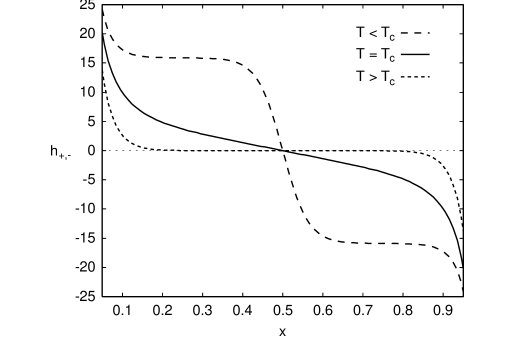
FIG. 7.: Scaling function $h_{+,-}(x;y)$ for $T<T_{c}$ $(y<0)$ (long dashed line), $T=T_{c}$ $(y=0)$ (solid line), and $T>T_{c}$ $(y>0)$ (short dashed line) according to Eq. (A31) as a function of $x$. $T_{c}$ denotes the bulk critical temperature. For $y\neq 0$ the thick-film limit $(|y|\gg 1)$ is shown (see main text).

One obtains

$$h_{+,+}(x;y)=2K{\mbox{dn}(2Kx;k)\over\mbox{sn}(2Kx;k)} \quad,\quad y=(2K)^{2}(2k^{2}-1),$$ (A28)

$$h_{+,+}(x;y)=2K{1\over\mbox{sn}(2Kx;k)} \quad,\quad y=-(2K)^{2}(k^{2}+1),$$ (A30)

and

$$h_{+,-}(x;y)=2K{\mbox{cn}(2Kx;k)\over\mbox{sn}(2Kx;k)\mbox{dn}(2Kx;k)} \quad,\quad y=-2(2K)^{2}(2k^{2}-1),$$ (A31)

$$h_{+,-}(x;y)=2K{\mbox{cn}(2Kx;k)\mbox{dn}(2Kx;k)\over\mbox{sn}(2Kx;k)} \quad,\quad y=2(2K)^{2}(k^{2}+1).$$ (A33)

The functional forms of $h_{+,+}$ and $h_{+,-}$ below, at, and above bulk criticality are displayed in Figs. 6 and 7, respectively. Bulk criticality means $y=0$, i.e., $k^{2}=1/2$ and off bulk criticality the thick film limit $|y|\gg 1$ $(k\to 1)$ is shown. In terms of the bulk correlation length $\xi$ the limit $|y|\gg 1$ in Figs.6 and 7 is represented as $L/\xi>15$.

B Eigenmode spectra

The Gaussian Hamiltonian given by Eq. (49) can be conveniently diagonalized by solving the eigenvalue problem

$$-\nabla^{2}\Psi({\bf x},z)+l(l+1)m^{2}(z)\Psi({\bf x},z)=E\Psi({\bf x},z),$$ (B1)

where $l=1$ for the transverse spectrum and $l=2$ for the longitudinal spectrum and $0\leq z\leq L$. The film geometry is homogeneous and isotropic with respect to ${\bf x}$ so that we can write $\Psi({\bf x},z)$ in the product form

$$\Psi({\bf x},z)=(2\pi)^{-(d-1)/2}e^{i{\bf p}\cdot{\bf x}}\psi_{n}^{(l)}(z),$$ (B2)

where ${\bf p}$ is the longitudinal momentum and $\psi_{n}^{(l)}(z)$ solves the eigenvalue equation

$$-{d^{2}\over dz^{2}}\psi_{n}^{(l)}(z)+l(l+1)m^{2}(z)\psi_{n}^{(l)}(z)=\epsilon_{n}^{(l)}\psi_{n}^{(l)}(z)$$ (B3)

so that the eigenvalue $E$ in Eq. (B1) takes the form $E={\bf p}^{2}+\epsilon_{n}^{(l)}$ for $l=1$ and $l=2$, respectively. As shown in Eqs. (A6) and (A7) $m^{2}(z)$ is given by the Weierstrass elliptic function $\wp(z)\equiv\wp(z;g_{2},g_{3})$, where $g_{3}=0$ for the case $\tau=0$ considered here [see Eq. (A8)]. Therefore Eq. (B3) is identical to the well known Lamé differential equation [54] written in the form of an eigenvalue problem. The solutions of Eq. (B3) are known for $l=1$ and $l=2$ and can be used to construct the eigenfunctions $\psi_{n}^{(l)}(z)$. Note that due to $m^{2}(z)=\wp(z)\sim 1/z^{2}$ for $z\to 0$ one has $\psi_{n}^{(l)}(z)\sim z^{l+1}$ for $z\to 0$ by inspection of Eq. (B3). Furthermore, $(+,+)$ and $(+,-)$ boundary conditions can be treated on the same footing by noting that according to Eqs. (A14) and (A23) one has

$$\omega_{1}^{(++)}=L/2 \ ,\ \omega_{2}^{(++)}=iL/2,$$ (B4)

$$\omega_{1}^{(+-)}=(1-i)L/4 \ ,\ \omega_{2}^{(+-)}=(1+i)L/4$$ (B5)

for the basic semiperiods of the Weierstrass function. The spectra for the cases $(SB,+)$ and $(O,+)$ can be constructed from the spectra for $(+,+)$ and $(+,-)$ boundary conditions, respectively.

First we turn to the transverse spectrum . According to Ref. [54] the eigenfunctions $\psi_{n}^{(1)}(z)$ up to a normalization constant can be written in the form

$$\psi_{n}^{(1)}(z)=\left[\sigma(z+\alpha_{n})e^{-z\zeta(\alpha_{n})}+\sigma(z-\alpha_{n})e^{z\zeta(\alpha_{n})}\right]/\sigma(z),$$ (B6)

where

$$\epsilon_{n}^{(1)}=-\wp(\alpha_{n})$$ (B7)

yields the eigenvalues and $\zeta(z)$ and $\sigma(z)$ are the Weierstrass $\zeta$ and $\sigma$ functions, respectively [53]. The spectral parameter $\alpha_{n}$ can be obtained from the requirement $\psi_{n}^{(1)}(z)=\pm\psi_{n}^{(1)}(z+L)$, i.e., the eigenfunctions are either even or odd functions when continued analytically to the interval $[-L,L]$. From Eq. (B4) one has $L=2\omega_{1}^{(++)}=2(\omega_{1}^{(+-)}+\omega_{2}^{(+-)})$ and using the shift properties of $\sigma(z)$ [53] the above shift operation can be directly applied to Eq. (B6). One obtains for the eigenvalue spectrum

$$2\alpha_{n}\zeta(L/2)-L\zeta(\alpha_{n})=n\pi i\ ,\ \epsilon_{n}^{(1)}=-\wp(\alpha_{n})\ ,\ n\geq 2,$$ (B8)

where the lower bound on the mode index $n$ comes from the requirement $\psi_{n}^{(1)}(z)\sim z^{2}$ for $z\to 0$ for the transverse eigenfunctions (see above).

For the longitudinal spectrum $(l=2)$ the eigenfunctions take the form [54]

$$\psi_{n}^{(2)}(z)={d\over dz}\left\{\left[\sigma(z+\alpha_{n})e^{-z[\zeta(\alpha_{n})+\beta_{n}]}+\sigma(z-\alpha_{n})e^{z[\zeta(\alpha_{n})+\beta_{n}]}\right]/\sigma(z)\right\},$$ (B9)

where

$$\beta_{n}={\wp^{\prime}(\alpha_{n})\over 2\wp(\alpha_{n})+\epsilon_{n}^{(2)}/3}\quad,\quad\wp(\alpha_{n})={(\epsilon_{n}^{(2)})^{3}\over 27g_{2}-9(\epsilon_{n}^{(2)})^{2}}$$ (B10)

yields the eigenvalues and $\wp^{\prime}(z)$ denotes the derivative of the Weierstrass $\wp$-function with respect to $z$. We again employ the symmetry requirement $\psi_{n}^{(2)}(z)=\pm\psi_{n}^{(2)}(z+L)$ and the boundary behavior $\psi_{n}^{(2)}(z)\sim z^{3}$ for $z\to 0$ to obtain

$$2\alpha_{n}\zeta(L/2)-L\left[\zeta(\alpha_{n})+{\wp^{\prime}(\alpha_{n})\over 2\wp(\alpha_{n})+\epsilon_{n}^{(2)}/3}\right]=n\pi i\ ,\ \wp(\alpha_{n})={(\epsilon_{n}^{(2)})^{3}\over 27g_{2}-9(\epsilon_{n}^{(2)})^{2}}\ ,\ n\geq 3.$$ (B11)

The solution of Eqs. (B8) and (B11) for the eigenvalues $\epsilon_{n}^{(i)}$, $i=1,2$ cannot be obtained in a closed analytic form. In order to deal with the divergencies of the mode sums in Eqs. (51) and (52) (see also Appendix C), we derive the asymptotic behavior of the eigenvalues from Eqs. (B8) and (B11) for large $n$. From the geometry of the problem it is clear that the leading term in an expansion of $\epsilon_{n}^{(i)}$ in powers of $1/n$ is given by the spectrum $(n\pi/L)^{2}$ of a free particle in a one-dimensional box of length $L$. Therefore the spectral parameter $\alpha_{n}$ behaves as $1/n$ as $n$ increases, so that the desired asymptotic form of the $n$ dependence of the eigenvalues can be obtained from Eqs. (B8) and (B11) by expanding the Weierstrass functions $\zeta(\alpha_{n})$, $\wp(\alpha_{n})$, and $\wp^{\prime}(\alpha_{n})$ in powers of $\alpha_{n}$, where only the leading two terms are needed. Specifically, we use the expansions [53]

$$\zeta(x)=1/x-g_{2}/60\ x^{3}+{\cal O}(x^{7})\ ,\ \wp(x)=1/x^{2}+g_{2}/20\ x^{2}+{\cal O}(x^{6}),$$ (B12)

where $g_{3}=0$ is implicitly assumed. The calculation is straightforward so that we only briefly summarize the results for the eigenvalues $\epsilon_{n}^{(i)}$. Corresponding expansions are obtained for the spectral parameter $\alpha_{n}$ which will not be reproduced here.

For $(+,+)$ boundary conditions one has

$$\zeta(L/2)=\zeta(\omega_{1}^{(++)})=\pi/(2L)\ ,\ g_{2}=-4t_{\perp\perp}=(2K/L)^{4},$$ (B13)

where $K=K(1/\sqrt{2})$ [see Eqs. (A8), (10), and (11)]. By insertion of Eqs. (B12) and (B13) into Eqs. (B8) and (B11) one obtains the expansions

$$\epsilon_{n}^{(1)} = \left({n\pi\over L}\right)^{2}\left[1-{2\over\pi n^{2}}+{1\over\pi^{2}n^{4}}\left({4K^{4}\over 3\pi^{2}}-1\right)+{\cal O}(n^{-6})\right]\ ,\ (n\geq 2)$$ (B14)

$$\epsilon_{n}^{(2)} = \left({n\pi\over L}\right)^{2}\left[1-{6\over\pi n^{2}}+{9\over\pi^{2}n^{4}}\left({4K^{4}\over 3\pi^{2}}-1\right)+{\cal O}(n^{-6})\right]\ ,\ (n\geq 3).$$ (B16)

For $(+,-)$ boundary conditions one has correspondingly

$$\zeta(L/2)=\zeta(\omega_{1}^{(+-)}+\omega_{2}^{(+-)})=\pi/L\ ,\ g_{2}=-4t_{\perp\perp}=-4(2K/L)^{4},$$ (B17)

where $K$ is given as above [see Eqs. (A8), (10), and (13)]. Insertion of Eqs. (B12) and (B17) into Eqs. (B8) and (B11) yields the expansions

$$\epsilon_{n}^{(1)} = \left({n\pi\over L}\right)^{2}\left[1-{4\over\pi n^{2}}-{4\over\pi^{2}n^{4}}\left({4K^{4}\over 3\pi^{2}}+1\right)+{\cal O}(n^{-6})\right]\ ,\ (n\geq 2)$$ (B18)

$$\epsilon_{n}^{(2)} = \left({n\pi\over L}\right)^{2}\left[1-{12\over\pi n^{2}}-{36\over\pi^{2}n^{4}}\left({4K^{4}\over 3\pi^{2}}+1\right)+{\cal O}(n^{-6})\right]\ ,\ (n\geq 3).$$ (B20)

The asymptotic expressions for the spectrum given by Eqs. (B14) and (B18) capture all divergent terms in the mode sums in Eqs. (51) and (52) as will be seen in Appendix C. Furthermore, Eqs. (B14) and (B18) provide very good initial values for a numerical solution of Eqs. (B8) and (B11) by iterative schemes, e.g., the Newton procedure.

For $(SB,+)$ boundary conditions the eigenvalue spectra can be obtained from the case of $(+,+)$ boundary conditions by employing the transformation $L\to 2L$ and by allowing only even indices $n$ for $\epsilon_{n}^{(1)}$ and only odd indices $n$ for $\epsilon_{n}^{(2)}$ [see Eq. (C17)]. Likewise, the eigenvalue spectra for $(O,+)$ boundary conditions can be obtained from the case of $(+,-)$ boundary conditions by again employing the transformation $L\to 2L$ and by allowing only odd indices $n$ for $\epsilon_{n}^{(1)}$ and only even indices $n$ for $\epsilon_{n}^{(2)}$ [see Eq. (C24)]. The reason for this simple rule is that for $(+,+)$ boundary conditions starting from the ground state every second eigenfunction has vanishing slope at $z=L/2$ so that after rescaling $L\to 2L$ the eigenfunctions for $(SB,+)$ boundary conditions are already contained in the $(+,+)$ case. An analogous argument relates the spectra for $(+,-)$ and $(O,+)$ boundary conditions starting from the first excited state for the $(+,-)$ case.

C Regularized mode sums

The mode sums appearing in Eqs. (51) and (52) are divergent for any spatial dimension $d$ of interest. Within the dimensional regularization scheme used throughout this investigation $d$ is used as a free parameter in order to find an analytic continuation of the mode sums as a function of $d$, where $d=4-\varepsilon$ is this case. On the other hand the mode sums in Eqs. (51) and (52) also constitute the zeta functions of the eigenvalue spectrum with a $d$ dependent argument [55]. The zeta function regularization of mode sums, which is a widely used technique to treat divergent series like those in Eqs. (51) and (52) [55], is therefore equivalent to the dimensional regularization scheme.

The major obstacle towards an analytical treatment of the aforementioned mode sums has been removed in Appendix B by the derivation of the asymptotic behavior of the eigenvalue spectrum for large mode numbers given by Eqs. (B14) and (B18). Using these results one has for $i=1,2$

$$\sum_{n=n_{0}}^{\infty}\left\{(\epsilon_{n}^{(i)})^{(d-1)/2}-\left[{n\pi\over L}\right]^{d-1}\left[1-{2A\over n^{2}}+{B\over n^{4}}\right]^{(d-1)/2}\right\}\sim\sum_{n=n_{0}}^{\infty}n^{d-7}$$ (C1)

which is convergent for any $d$ of physical interest and can thus be determined numerically from the solutions of Eqs. (B8) and (B11) for the transverse and the longitudinal mode sum, respectively. The problem of regularizing the mode sums has therefore reduced to the regularization of the corresponding sums over the large $n$ expansions given by Eqs. (B14) and (B18), i.e., one has to consider the series

$$\sum_{n=n_{0}}^{\infty}n^{d-1}\left[1-{2A\over n^{2}}+{B\over n^{4}}\right]^{(d-1)/2}$$ (C2)

for $d=4-\varepsilon$. If the lower summation bound $n_{0}$ in Eq. (C2) is chosen sufficiently large, one can safely expand the term under the sum in powers of $1/n^{2}$ which leads to an expansion of the series given by Eq. (C2) in terms of Hurwitz functions $\zeta(x,n_{0})$. One finds for $d=4-\varepsilon$

$$\sum_{n=n_{0}}^{\infty}\left[n^{2}-2A+{B\over n^{2}}\right]^{(3-\varepsilon)/2} = \zeta(-3,n_{0})-3A\zeta(-1,n_{0})$$ (C3)

$$+ {3-\varepsilon\over 2}\left[(1-\varepsilon)A^{2}+B\right]\zeta(1+\varepsilon,n_{0})$$ (C5)

$$+ {A\over 2}(A^{2}-3B)\zeta(3,n_{0})+{3\over 8}(A^{2}-B)^{2}\zeta(5,n_{0})$$ (C7)

$$+ {3\over 8}A(A^{2}-B)^{2}\zeta(7,n_{0})+{\cal O}(\varepsilon)+{\cal O}(1/n_{0}^{8}),$$ (C9)

where the $\varepsilon$-expansion has already been carried out up to terms ${\cal O}(\varepsilon)$. The expansion shown in Eq. (C3) converges quite fast already for $3\leq n_{0}\leq 5$. The $1/\varepsilon$ pole indicating the UV singularity can be extracted from Eq. (C3) using the expansion

$$\zeta(1+\varepsilon,n_{0})=1/\varepsilon+\gamma-\sum_{k=1}^{n_{0}-1}1/k+{\cal O}(\varepsilon),$$ (C10)

where $\gamma\simeq 0.577216$ is the Euler constant and $n_{0}$ is a positive integer. With the coefficients $A$ and $B$ taken from Eqs. (B14) and (B18) the expressions given by Eqs. (C1), (C3), and (C10) can be combined to the following regularized and $\varepsilon$-expanded expressions for the mode sums.

For $(+,+)$ boundary conditions one finds with $K\equiv K(1/\sqrt{2})$

$$\sum_{n=2}^{\infty}\left(\epsilon_{n}^{(1)}\right)^{(d-1)/2} = \left[\pi\over L\right]^{d-1}{2K^{4}\over\pi^{4}\varepsilon}\left[1-\varepsilon\left({3\pi^{2}\over 4K^{4}}+{1\over 3}-\gamma+0.7494\right)\right]+{\cal O}(\varepsilon),$$ (C11)

$$\sum_{n=3}^{\infty}\left(\epsilon_{n}^{(2)}\right)^{(d-1)/2} = \left[\pi\over L\right]^{d-1}{18K^{4}\over\pi^{4}\varepsilon}\left[1-\varepsilon\left({3\pi^{2}\over 4K^{4}}+{1\over 3}-\gamma+1.5589\right)\right]+{\cal O}(\varepsilon).$$ (C13)

For $(+,-)$ boundary conditions the corresponding result reads

$$\sum_{n=2}^{\infty}\left(\epsilon_{n}^{(1)}\right)^{(d-1)/2} = -\left[\pi\over L\right]^{d-1}{8K^{4}\over\pi^{4}\varepsilon}\left[1+\varepsilon\left({3\pi^{2}\over 4K^{4}}-{1\over 3}+\gamma-1.7198\right)\right]+{\cal O}(\varepsilon),$$ (C14)

$$\sum_{n=3}^{\infty}\left(\epsilon_{n}^{(2)}\right)^{(d-1)/2} = -\left[\pi\over L\right]^{d-1}{72K^{4}\over\pi^{4}\varepsilon}\left[1+\varepsilon\left({3\pi^{2}\over 4K^{4}}-{1\over 3}+\gamma-2.4086\right)\right]+{\cal O}(\varepsilon).$$ (C16)

For $(SB,+)$ boundary conditions we apply the simple transformation described in the last paragraph of Appendix B to the eigenvalue spectrum for $(+,+)$ boundary conditions. From Eq. (B14) we find the expansions

$$\epsilon_{n}^{(1)} = \left({n\pi\over L}\right)^{2}\left[1-{1\over 2\pi n^{2}}+{1\over 16\pi^{2}n^{4}}\left({4K^{4}\over 3\pi^{2}}-1\right)+{\cal O}(n^{-6})\right]\ ,\ (n\geq 1)$$ (C17)

$$\epsilon_{n}^{(2)} = \left({(2n+1)\pi\over 2L}\right)^{2}\left[1-{6\over\pi(2n+1)^{2}}+{9\over\pi^{2}(2n+1)^{4}}\left({4K^{4}\over 3\pi^{2}}-1\right)+{\cal O}(n^{-6})\right]\ ,\ (n\geq 1),$$ (C19)

for the transverse and the longitudinal spectrum, respectively. Due to the appearance of half-integer arguments in the Hurwitz functions for the transverse mode sum in this case one needs the expansion

$$\zeta(1+\varepsilon,3/2)=1/\varepsilon+\gamma+2\ln 2-2+{\cal O}(\varepsilon)$$ (C20)

instead of Eq. (C10). Furthermore, the r.h.s. of Eq. (C3) with $n_{0}$ replaced by $3/2$ is needed in order to derive the regularized longitudinal mode sum. The transverse mode sum, however, can be evaluated directly using Eqs. (C3) and (C10). One therefore finds for $(SB,+)$ boundary conditions

$$\sum_{n=1}^{\infty}\left(\epsilon_{n}^{(1)}\right)^{(d-1)/2} = \left[\pi\over L\right]^{d-1}{K^{4}\over 8\pi^{4}\varepsilon}\left[1-\varepsilon\left({3\pi^{2}\over 4K^{4}}+{1\over 3}-\gamma-1.9712\right)\right]+{\cal O}(\varepsilon),$$ (C21)

$$\sum_{n=1}^{\infty}\left(\epsilon_{n}^{(2)}\right)^{(d-1)/2} = \left[\pi\over L\right]^{d-1}{9K^{4}\over 8\pi^{4}\varepsilon}\left[1-\varepsilon\left({3\pi^{2}\over 4K^{4}}+{1\over 3}-\gamma-0.8405\right)\right]+{\cal O}(\varepsilon).$$ (C23)

For $(O,+)$ boundary conditions we apply the same transformation to the eigenvalue spectrum for $(+,-)$ boundary conditions. From Eq. (B18) we find the expansions

$$\epsilon_{n}^{(1)} = \left({(2n+1)\pi\over 2L}\right)^{2}\left[1-{4\over\pi(2n+1)^{2}}-{4\over\pi^{2}(2n+1)^{4}}\left({4K^{4}\over 3\pi^{2}}+1\right)+{\cal O}(n^{-6})\right]\ ,\ (n\geq 1)$$ (C24)

$$\epsilon_{n}^{(2)} = \left({n\pi\over L}\right)^{2}\left[1-{3\over\pi n^{2}}-{9\over 4\pi^{2}n^{4}}\left({4K^{4}\over 3\pi^{2}}+1\right)+{\cal O}(n^{-6})\right]\ ,\ (n\geq 2),$$ (C26)

Using Eq. (C3) with $n_{0}$ replaced by $3/2$ in order to evaluate the transverse mode sum one therefore finds for $(O,+)$ boundary conditions

$$\sum_{n=1}^{\infty}\left(\epsilon_{n}^{(1)}\right)^{(d-1)/2} = -\left[\pi\over L\right]^{d-1}{K^{4}\over 2\pi^{4}\varepsilon}\left[1+\varepsilon\left({3\pi^{2}\over 4K^{4}}-{1\over 3}+\gamma-1.8975\right)\right]+{\cal O}(\varepsilon),$$ (C27)

$$\sum_{n=2}^{\infty}\left(\epsilon_{n}^{(2)}\right)^{(d-1)/2} = -\left[\pi\over L\right]^{d-1}{9K^{4}\over 2\pi^{4}\varepsilon}\left[1+\varepsilon\left({3\pi^{2}\over 4K^{4}}-{1\over 3}+\gamma-1.9276\right)\right]+{\cal O}(\varepsilon).$$ (C29)

In order to facilitate the $\varepsilon$-expansion of Eq. (52) we finally note that

$$\Gamma\left[(3-d)/2\right]=-2\sqrt{\pi}\left[1+\varepsilon(1-\ln 2-\gamma/2)+{\cal O}(\varepsilon^{2})\right]$$ (C30)

and

$$\Gamma(d/2)=1-\varepsilon(1-\gamma)/2+{\cal O}(\varepsilon^{2})$$ (C31)

for $d=4-\varepsilon$ (see also Ref. [28] for similar relations).

REFERENCES

- [1] K. Binder in Phase Transitions and Critical Phenomena, edited by C. Domb and J.L. Lebowitz (Academic, London, 1983), Vol.8, p. 2.
- [2] H.W. Diehl in Phase Transitions and Critical Phenomena, edited by C. Domb and J.L. Lebowitz (Academic, London, 1986), Vol.10, p. 76.
- [3] S. Dietrich in Phase Transitions and Critical Phenomena, edited by C. Domb and J.L. Lebowitz (Academic, London, 1988), Vol.12, p. 1.
- [4] M.E. Fisher and H. Au-Yang, Physica A 101A, 255 (1980).
- [5] H.W. Diehl and A. Ciach, Phys. Rev. B 44, 6642 (1991).
- [6] H.W. Diehl and M. Smock, Phys. Rev. B 47, 5841 (1993).
- [7] M.E. Fisher, in Proceedings of the 1970 Enrico Fermi School of Physics, Varenna, Italy, Course No. LI, edited by M.S. Green (Academic, New York, 1971), p. 1; M. E. Fisher and M.N. Barber, Phys. Rev. Lett. 28, 1516 (1972).
- [8] M.E. Fisher and H. Nakanishi, J. Chem. Phys. 75, 5857 (1981).
- [9] M.N. Barber, in Phase Transitions and Critical Phenomena, edited by C. Domb and J.L. Lebowitz (Academic, New York, 1983), Vol. 8, p. 145; V. Privman, in Finite Size Scaling and Numerical Simulation of Statistical Systems, edited by V. Privman (World Scientific, Singapore, 1990).
- [10] M.P. Nightingale and J.O. Indekeu, Phys. Rev. Lett. 54, 1824 (1985) and Phys. Rev. Lett. 55, 1700 (1985); R. Lipowski and U. Seifert, Phys. Rev. B 31, 4701 (1985) and Phys. Rev. Lett. 55, 1699 (1985).
- [11] H. Nakanishi and M.E. Fisher, J. Chem. Phys. 79, 3279 (1983).
- [12] K. Binder and D.P. Landau, Physica A 177, 483 (1991).
- [13] R. Evans, U. Marini Bettolo Marconi, and P. Tarazona, J. Chem. Phys. 84, 2376 (1986).
- [14] A.O. Parry and R. Evans, J. Phys. A 25, 275 (1992).
- [15] K. Binder and D.P. Landau, J. Chem. Phys. 96, 1444 (1992).
- [16] M.R. Swift, A.L. Owczarek, and J.O. Indekeu, Europhys. Lett. 14, 475 (1991).
- [17] A.O. Parry and R. Evans, Physica A 181, 250 (1992).
- [18] K. Binder, D.P. Landau, and A.M. Ferrenberg, Phys. Rev. Lett. 74, 298 (1995).
- [19] A.O. Parry, J. Phys. A 25, 257 (1992).
- [20] K. Binder, R. Evans, D.P. Landau, and A.M. Ferrenberg, Phys. Rev. E 53, 5023 (1996).
- [21] M. Krech, The Casimir Effect in Critical Systems (World Scientific, Singapore, 1994) and references therein.
- [22] L. Spruch, Science 272, 1452 (1996) and references therein.
- [23] S.L. Carnie, D.Y.C. Chan, and J. Stankovich, J. Coll. Int. Sci. 169, 116 (1994).
- [24] G.H. Nyland and I. Brevik, Physica A 202, 81 (1994); I. Brevik and G.H. Nyland, Ann. Phys. 230, 321 (1994).
- [25] S. Leseduarte and A. Romeo, Ann. Phys. 250, 448 (1996).
- [26] M.Y. Novikov, A.S. Sorin, and V.Y. Chernyak, Theor. Math. Phys. 91, 658 (1992) and 92, 773 (1993).
- [27] M. Borday, G.L. Klimchitskaya, and V.M. Mostepanenko, Phys. Lett. A 200, 95 (1995).
- [28] M. Krech and S. Dietrich, Phys. Rev. A 46, 1886 (1992).
- [29] J.L. Cardy, Nucl. Phys. bf B275, 200 (1986).
- [30] R. Evans and J. Stecki, Phys. Rev. B 49, 8842 (1994).
- [31] D. Danchev, Phys. Rev. E 53, 2104 (1996).
- [32] J.O. Indekeu, M.P. Nightingale, and W.V. Wang, Phys. Rev. B 34, 330 (1986).
- [33] M. Krech and D.P. Landau, Phys. Rev. E 53, 4414 (1996).
- [34] T.W. Burkhardt and E. Eisenriegler, Phys. Rev. Lett. 74, 3189 (1995); E. Eisenriegler and U. Ritschel, Phys. Rev. B 51, 13717 (1995).
- [35] D. O’Connor and C.R. Stephens, Phys. Rev. Lett. 72, 506 (1994); F. Freire, D. O’Connor, and C.R. Stephens, J. Stat. Phys. 74, 219 (1994).
- [36] A. Esser, V. Dohm, and X.S. Chen, Physica A 222, 355 (1995); A. Esser, V. Dohm, M. Hermes, and J.S. Wang, Z. Phys. B 97, 205 (1995); X.S. Chen, V. Dohm, and A.L. Talapov, Physica A 232, 375 (1996).
- [37] X.S. Chen, V. Dohm, and A. Esser, J. Phys. I France 5, 205 (1995); X.S. Chen, V. Dohm, and N. Schultka, Phys. Rev. Lett. 77, 3641 (1996).
- [38] M.I. Kaganov and A.N. Omel’yanchuk, Sov. Phys. JETP 34, 895 (1972); M.I. Kaganov, Sov. Phys. JETP 35, 631 (1972).
- [39] E. Brézin, F. Korutcheva, T. Jolicoeur, and J. Zinn-Justin, J. Stat. Phys. 70, 583 (1993).
- [40] S. Gnutzmann and U. Ritschel, Z. Phys. B 96, 391 (1995).
- [41] G. Gumbs, J. Math. Phys. 24, 202 (1983).
- [42] T.W. Burkhardt and H.W. Diehl, Phys. Rev. B 50, 3894 (1994).
- [43] C. Ruge, S. Dunkelmann, and F. Wagner, Phys. Rev. Lett. 69, 2465 (1992); C. Ruge and F. Wagner, Phys. Rev. B 52, 4209 (1995).
- [44] E. Eisenriegler and M. Stapper, Phys. Rev. B 50, 10009 (1994).
- [45] J. Rudnick, H. Guo, and D. Jasnow, J. Stat. Phys. 41, 353 (1985).
- [46] H. Kleinert, J. Neu, V. Schulte-Frohlinde, K.G. Chetyrkin, and S.A. Larin, Phys. Lett. B 272, 39 (1991).
- [47] A.M. Ferrenberg and R.H. Swendsen, Phys. Rev. Lett. 63, 1195 (1989).
- [48] M. Krech and S. Dietrich, Phys. Rev. A 46, 1922 (1992).
- [49] S. Dietrich and A. Latz, Phys. Rev. B 40, 9204 (1989).
- [50] E.S. Sabisky and C.H. Anderson, Phys. Rev. A 7, 790 (1973).
- [51] A. Mukhopadhyay and B.M. Law, private communication.
- [52] J.N. Israelachvili and P.M. McGuggian, Science 241, 795 (1988) and references therein.
- [53] L.S. Gradsteyn and I.M. Ryzhik, Table of Integrals, Series and Products (Academic, New York, 1980), pp. 904.
- [54] E. Kamke, Differentialgleichungen, Lösungsmethoden und Lösungen (Chelsea, New York, 1971), Vol. 1, pp. 408.
- [55] E. Elizalde, J. Phys. A 27, L299 (1994) and references therein.