Temperature evolution and bifurcations of metastable states in mean-field spin glasses, with connections with structural glasses

Abstract

The correlations of the free-energy landscape of mean-field spin glasses at different temperatures are investigated, concentrating on models with a first order freezing transition. Using a “potential function” we follow the metastable states of the model in temperature, and discuss the possibility of level crossing (which we do not find) and multifurcation (which we find). The dynamics at a given temperature starting from an equilibrium configuration at a different temperature is also discussed. In presence of multifurcation, we find that the equilibrium is never achieved, leading to aging behaviour at slower energy levels than usual aging. The relevance of the observed mechanisms for real structural glasses is discussed, and some numerical simulations of a soft sphere model of glass are presented.

I Introduction

Free-energy landscapes in high dimensional spaces have longly been used as metaphores for describing the physics of complex systems as glasses and spin-glasses, and also proteins and evolutionary fitness landscapes [2]. The basic idea of this approach is that complex systems dynamics can be viewed as a search for optima in a rough hypersurface. Although free-energy surfaces can in principle be defined for large classes of finite dimensional models, the actual construction of such functions has been achieved only in the case of long-range disordered system (mean-field spin glasses), which relevance for finite dimensional spin glasses has been subject of a long debate, growing evidence [3] pointing in the direction that mean-field theory is a good starting point to describe finite dimensional physics. Thouless Anderson and Palmer [4] (TAP) showed that stable and metastable states of long-range spin glasses are associated to minima of a suitable free-energy, which is a random function in a $N$ ($\to\infty$) dimensional space. The complex phenomenology of equilibrium spin-glasses can be read as a set of propositions about the low lying minima of the TAP free-energy, and the barriers separating them.

Due to the random character of the TAP free-energy function, analytic statements on the structure of the stationary point have forcedly statistical character. Various techniques have been invented to study the minima of TAP free-energy, and the structure of the stable and metastable minima for fixed external parameter is known in great detail, and gives a coherent picture of the glassy transition. Two classes of models are known, according to the order of the freezing transition. In models like the Sherrington-Kirkpatrick models, which display a second order phase transition, the metastable states of the TAP free-energy do not play an important physical role. A second order transition suggests a mechanism of bifurcation (or rather multifurcation) of the paramagnetic minimum as $T_{c}$ is crossed. In off-equilibrium dynamics it is found that all the extensive quantities tend to their equilibrium values for large times. Whereas these mean-field models, with continuous transition, seem to apply for the description of real spin glasses, a second class of models, like e.g. the Potts glass, show a first order freezing transition, and seem closer to describing the physics of structural glasses. Indeed, for these models occurs a purely dynamical transition where the relaxation time diverges, while the static thermodynamic quantities show singularities only at a lower temperature. Below the dynamical transition temperature, metastable states dominate the physics, and, dynamically, the extensive quantities do not tend to their equilibrium values if a random initial condition is chosen. Statically, the partition function is dominated by metastable states (between the statical and the dynamical transitions, by an exponentially large number of mutually inaccessible states) that the system is unable to reach dynamically.

The scenario in which the barriers between metastable states are infinite, and where a quenched system never reaches any of these states, is clearly linked to the mean-field approximation. For finite systems, metastable states have a finite lifetime, and the system should be able to find them in a finite time. This time, and the states the system is able to find, can depend for example on the cooling rate. A modified scenario would include “activated processes” and suppress the divergence of relaxation times at the dynamical transition, replacing it by a rapid increase (with divergence only at the static transition).

This picture, as was already advocated in [5, 6, 7] and more recently in [8], could be relevant for real glasses: indeed, the glass transition temperature is also a purely dynamical quantity, defined by the fact that the relaxation time reaches a certain value, the existence of a static transition at a lower temperature still being subject of debate. Below this temperature, the system remains out of equilibrium for all available time scales, and static quantities are not reached. In the same way, the aforementioned scenario would yield a glass transition (corresponding to a large but finite value of the relaxation time) occuring above the static transition, and a dynamical evolution resulting from a mixture of mean-field like dynamics and activated processes.

In this context, the relevance of mean-field studies depends on the various time scales involved: if the barriers between metastable states are low, activated processes are fast and will dominate the evolution; if on the contrary the energy barriers are finite but large, there will exist time windows in which the mean-field scenario will hold.

To address this question, we have therefore to gain knowledge on the metastable states, both statically and dynamically, for the mean-field models, and to compare the emerging picture and dynamical scenarios with the real world, or at least with numerical simulations.

If the structure of the TAP minima for fixed temperature is rather well known [9, 10], a much less coherent picture is available for the correlation of the free-energy landscapes for different temperatures. In the Sherrington-Kirkpatrick model, the study of [11, 12] have revealed “chaotic temperature dependence” of the low lying states. States of equilibrium at different temperatures are, no matter how small the temperature differences, as uncorrelated as they can. In some other models the chaotic property is absent. A clear example is the spherical $p$-spin model, where the homogeneity of the Hamiltonian implies that the order of the free-energy minima does not depend on temperature, so that, in the whole low-temperature phase, the statics is given by the same low-lying states. Some general conclusions about the fate of TAP minima under temperature changes can be drawn on the basis of smoothness of the TAP free-energy as a function of temperature. For example, absolutely stable minima can not disappear or multifurcate for an infinitesimal change of the temperature, and the generation of new stationary points has to pass by a marginally stable situation.

Two issues appear to be relevant for the description of correlations of the landscapes for different temperatures: level bifurcations and level crossing. Therefore, in this paper we try to gain some generic insights on these topics, by addressing the issue of following the TAP states in temperature for a spherical model which displays first order glassy transition. Differently from the $p$-spin model, the Hamiltonian is not homogeneous. We expect therefore that its behavior is generic in the class of models with first order transition. The analysis is performed with the aid of a recent method where the metastable states are associated to local minima of some macroscopic “potential” function of the spin-glass order parameter. The basic idea of this approach is that the free-energy manifold can be probed introducing an external field pointing in the direction of some typical equilibrium configuration [13, 14, 15]. In section two, we review the construction of the potential of ref. [13] and extend the discussion to some properties not mentioned there. In section three we use this potential to follow metastable states in temperature, and discuss the possibility of multifurcation.

In section four, we use another powerful approach, a dynamical one, with appropriate initial conditions: the dynamics of a system thermalized at a certain temperature, and then brought at another, also allows to explore the phase space of the system [13, 16]. We show that the two methods yield the same results, and use moreover this dynamical study to tackle another relevant issue: the dynamical behavior of the systems when a TAP solution bifurcates. In particular the problem whether the system will fall into one of the new valleys or will be unable to decide where to fall and age forever.

After having described these mechanisms for the considered mean-field models, we tentatively compare them in section five to the case of real glasses, via numerical simulations of a soft sphere glass. In particular, the dynamical mean-field approach of thermalized initial conditions can be thought of as a previous very slow cooling to a certain temperature, followed by a rapid change. The study of the energy reached with various cooling rates in the simulated system shows the relevance of the mean-field scenario, in the available time window.

II Studied models; the potential; previous results

The class of models we consider is defined by $N$ (real) spins ${\bf{s}}=\{s_{1},\cdots,s_{N}\}$ interacting through a Hamiltonian $H({\bf{s}})$ and a global (spherical) constraint $\sum_{i}s_{i}^{2}=N$. The Hamiltonian is random, Gaussian, with correlations

$$\overline{H({\bf{s}})H({\bf{s^{\prime}}})}=Nf(q_{\bf{ss^{\prime}}}),$$ (1)

where $q_{\bf{ss^{\prime}}}=1/N\sum_{i}s_{i}s^{\prime}_{i}$ is the overlap between the configurations ${\bf{s}}$ and ${\bf{s^{\prime}}}$. If $f$ is a polynomial function, the Hamiltonian can be presented as a linear combination of terms of the type

$$H_{p}({\bf{s}})=-\sum_{1\leq i_{1}<i_{2}\cdots<i_{p}\leq N}J_{i_{1}i_{2}\cdots i_{p}}s_{i_{1}}s_{i_{2}}\cdots s_{i_{p}},$$ (2)

with Gaussian independent couplings $J_{i_{1}i_{2}\cdots i_{p}}$, with zero mean and variance $p!/(2N^{p-1})$. It is easy to see that $\overline{H_{p}({\bf{s}})H_{p^{\prime}}({\bf{s^{\prime}}})}=\delta_{p,p^{\prime}}q_{\bf{ss^{\prime}}}^{p}/2$. As we will see in the following, the purely monomial case, the so called $p$-spin model, has remarkably simple properties under temperature changes [10] thanks to the homogeneity of the Hamiltonian under contemporary rescaling of all the variables. In order to study the generic behavior it is therefore necessary to consider inhomogeneous Hamiltonian, giving rise to non monomial correlation functions. The specific form of the function $f(q)$ we will use in our examples will be mainly $f(q)=1/2(q^{3}+q^{4})$, however the results will be generic for inhomogeneous Hamiltonian verifying the condition that $f^{\prime\prime}(q)^{-3/2}f^{\prime\prime\prime}(q)$ is monotonically decreasing with $q$ for all $q$ (this ensures that the transition is a discontinuous one).

In that case the statics of the model is described by

• a high temperature phase, for $T>T_{d}$, where the dominant contribution is given by a paramagnetic state;

• a temperature range $T_{d}>T>T_{s}$ where the replica calculations yield a replica symmetric result, which in fact corresponds to ergodicity breaking in an exponentially large number of states (finite complexity);

• a low temperature phase, for $T_{s}>T$, with a 1-step replica symmetry breaking, corresponding to the predominance of the lowest TAP states, with zero complexity.

The relaxation dynamics from a random initial state, yields equilibrium dynamics in the paramagnetic state for $T>T_{d}$, while, for $T_{d}>T$, the aging phenomena appears [17] and the long time limit of the energy per spin is higher than the equilibrium value.

In this section we review the construction of the potential function [13], and we expose some new results coming from a replica symmetry breaking Ansatz, which clarify some of the “mysteries” left open in [13].

A Construction of the potential

One of the characteristics of spin glasses, due to their random character, is that the different equilibrium states can not be selected by an external field uncorrelated with the landscape defined by the Hamiltonian. The basic idea underlying the potential function is to use an external field pointing in the direction of a particular equilibrium configuration [14, 13]. So, if ${\bf\sigma}_{i}$ denotes a typical equilibrium configuration at a temperature $T^{\prime}$ one can define the partition function

$$Z[T,\epsilon,{\bf\sigma}]=\sum_{S}{\rm e}^{-\beta H[S]+\epsilon S\cdot{\bf\sigma}}.$$ (3)

Besides being self-averaging with respect to the distribution of the quenched Hamiltonian, the free-energy $\Gamma[T,T^{\prime},\epsilon]=-T/N\log Z[T,\epsilon,{\bf\sigma}]$ is also independent on the particular configuration $\sigma$ we choose, and therefore coincide with its average over the probability distribution $\exp(-\beta^{\prime}H[{\bf\sigma}])/Z[T^{\prime}]$. We define the “potential” as the Legendre transform of $\Gamma$:

$$V[T,T^{\prime},q_{12}]=\min_{\epsilon}\Gamma[T,T^{\prime},\epsilon]+\epsilon q_{12}-F[T].$$ (4)

From the Legendre transform we have subtracted $F$ the free-energy at temperature $T$ in order to have $V[T,T^{\prime},0]=0$. Defined in this way, the potential has the meaning of the free-energy cost to keep a system at temperature $T$ at fixed overlap $q_{12}$ from a generic configuration of equilibrium at a different temperature $T^{\prime}$.

$V$ is self-averaging also with respect to the quenched disorder distribution, which we denote by an overline. The basic object we need to evaluate is then

$$\overline{{1\over Z[T^{\prime}]}\sum_{{\bf\sigma}}{\rm e}^{-\beta^{\prime}H[{\bf\sigma}]}\log\left(\sum_{S}{\rm e}^{-\beta H[S]+\epsilon S\cdot{\bf\sigma}}\right)},$$ (5)

As it is explained in detail in [13], in order to perform the averages it is possible to use a double analytic continuation from integer values of the parameters $m$ and $n$, used to represent $\log Z[T,\epsilon,\sigma]$ as $\lim_{m\to 0}(Z[T,\epsilon,\sigma]^{m}-1)/m$, and ${1/Z[T^{\prime}]}$ as $\lim_{n\to 0}Z^{n-1}$. There are then $n$ replicas ${\bf\sigma}_{a}$ ($a=1,...,n$), and $m$ replicas $S_{\alpha}$ ($\alpha=1,...,m$). The “external field” terms is an interaction term of all the replicas $S_{\alpha}$ with one privileged replica, say, ${\bf\sigma}_{1}$. Three overlap matrices turn out to be relevant for the description of the physics of the model: $Q^{*}_{ab}={1\over N}\sum_{i}\langle{\bf\sigma}^{a}_{i}{\bf\sigma}^{b}_{i}\rangle$ describing the overlap statistics of the replicas at equilibrium at temperature $T^{\prime}$, $P_{a,\alpha}={1\over N}\sum_{i}\langle{\bf\sigma}^{a}_{i}S^{\alpha}_{i}\rangle$ describing the overlaps among the replicas at temperature $T^{\prime}$ and the replicas at temperature $T$, and finally $Q^{\alpha\beta}={1\over N}\sum_{i}\langle S^{\alpha}_{i}S^{\beta}_{i}\rangle$ describing the overlaps between replicas at temperature $T$. As is physically clear, it is found that the structure of the matrix $Q^{*}_{ab}$ is not affected at the leading order by the presence of the replicas $S^{\alpha}$. In this paper we will restrict ourselves to the temperature range $T\geq T_{S}$, where $Q^{*}_{ab}=\delta_{ab}$. In this regime it is sensible to assume $P_{a,\alpha}=\delta_{a,1}q_{12}$ for all $\alpha$. The structure of the matrix $Q_{\alpha\beta}$ is more subtle. Assuming a single state picture in ref. [13] the form $Q_{\alpha\beta}=\delta_{\alpha\beta}+q(1-\delta_{\alpha\beta})$ was taken. But it turns out also to be necessary to consider the possibility that ergodicity is broken for the system in a “field”, with consequent replica symmetry breaking in $Q_{\alpha\beta}$. The most general Ansatz we shall need is the “one step” form (see e.g. [9]), characterized by the parameters $(q_{0},q_{1},x)$. With this Ansatz it easy to find that the potential as a function of all the order parameters is:

$$V(q_{12})=-\frac{1}{2\beta}\left\{2\beta\beta^{\prime}f(q_{12})-\beta^{2}\left((1-x)f(q_{1})+xf(q_{0})\right)+\frac{x-1}{x}{\rm ln}(1-q_{1})\right.$$ (6)

$$\left.+\frac{1}{x}{\rm ln}\left(1-(1-x)q_{1}-xq_{0}\right)+\frac{q_{0}-q_{12}^{2}}{1-(1-x)q_{1}-xq_{0}}\right\}$$ (7)

where $V$ has to be maximized with respect to $q_{0}$, $q_{1}$ and $x$. These saddle point equations read:

$$q_{12}^{2}=q_{0}-\beta^{2}f^{\prime}(q_{0})(1-(1-x)q_{1}-xq_{0})^{2},$$ (8)

$$\beta^{2}(f^{\prime}(q_{1})-f^{\prime}(q_{0}))(1-x)=(1-x)\frac{q_{1}-q_{0}}{(1-q_{1})(1-(1-x)q_{1}-xq_{0})},$$ (9)

$$\beta^{2}(f(q_{1})-f(q_{0}))+\frac{1}{x^{2}}{\rm ln}\left(\frac{1-q_{1}}{1-(1-x)q_{1}-xq_{0}}\right)+\beta^{2}\frac{(1-q_{1})}{x}f^{\prime}(q_{1})-\beta^{2}\frac{f^{\prime}(q_{0})}{x}(1-(1-x)q_{1}-xq_{0})=0.$$ (10)

A numerical resolution allows to construct the curve $V(q_{12})$ .

In general, this curve can be divided in three regions. There are a small and a large $q_{12}$ regions (outside the interval $A-B$ in figure 1) where replica symmetry holds. In between the symmetry is broken. In the large $q_{12}$ region, the solution is $q_{1}=q_{0}$ testifying ergodicity in a single state. In the point $B$ a de Almeida Thouless instability develops. The replica symmetry breaking region is interpreted as usual ergodicity breaking with dominance of small number of valleys for typical samples. In the point $A$ one finds $x=1$, and the restoring of replica symmetry implies in fact a number of valleys exponentially large ${\cal N}\sim{\rm e}^{N\Sigma(q_{12})}$. In this region (between $q_{12}=0$ and $A$), $x=1$, the Edwards-Anderson parameter inside the valleys is obtained as the value of $q_{1}$ from the second equation of (10) divided by $(1-x)$ in $x=1$, and is depicted with crosses in figure (2). The complexity $\Sigma(q_{12})$ can be calculated as in the usual case as ${\partial V\over\partial x}|_{x=1}$, and is depicted in figure (3). For $q_{12}=0$, where there is no effective constraint, the second replica is at equilibrium at $T$ and we find the total complexity at temperature $T$, and the equilibrium Edwards-Anderson parameter at $T$.

The global situation is displayed for a typical example in figures (1) and (2).

FIG. 1.: Potential $V$ as a function of $q_{12}$, for the $p=3+p=4$, $\beta=1.25$, $\beta^{\prime}=1.243$; full line: replica symmetric solution; dotted line: RSB solution, from A ($x=1$) to B (where $q_{0}$ and $q_{1}$ merge)

FIG. 2.: $q_{0}(q_{12}),q_{1}(q_{12})$ as a function of $q_{12}$, for the $p=3+p=4$, $\beta=1.25$, $\beta^{\prime}=1.243$ (lines); diamonds: RS solution, given by inserting $q_{0}=q_{1}$ in (10); crosses: continuation of $q_{1}(q_{12})$ in the first RS region, with $\lim_{q_{12}\to 0}q_{1}(q_{12})=q_{EA}(\beta)$

FIG. 3.: $\Sigma(q_{12})$ for the $p=3+p=4$, $\beta=1.25$, $\beta^{\prime}=1.243$; for $q_{12}\to 0$ we recover the complexity at $\beta$. In $A$ the complexity goes to zero, corresponding to the entrance in the RSB region of the potential.

B Minima of the potential

The qualitative features of the potential are largely independent of the form of the function $f$. Let us briefly discuss the case of equal temperatures $\beta=\beta^{\prime}$ [13]. The potential has always an absolute minimum for $q_{12}=0$, corresponding, as previously mentioned, to the second replica being at equilibrium. Another minimum appears for a non-zero value of $q_{12}$ for temperatures below $T_{d}$ (see figure (4)) (at $T=T^{\prime}=T_{d}$, it is a horizontal flex). This relative minimum corresponds to having both replicas in the same state, with $q_{12}=q=q_{EA}$. Since the number of equilibrium states at temperature $T$ is $\exp(N\Sigma(T))$ by definition of the complexity (or configurational entropy) $\Sigma$, the free energy cost of having this situation is

$$V_{relative\ minimum}(q_{EA})=T\Sigma(T)=-\frac{\beta}{2}f(q_{EA})-\frac{q_{EA}}{2\beta}-\frac{1}{2\beta}{\rm ln}(1-q_{EA}).$$ (11)

FIG. 4.: Potential $V$ as a function of $q_{12}$, for the $p=3$ $p$-spin model, for $\beta=\beta^{\prime}$, from top to bottom $\beta=1.6$, $\beta=\beta_{d}\approx 1.633$, $\beta=1.7$; here $\beta_{S}=1.706$

For the $p$-spin model, the case of different temperatures $\beta$ and $\beta^{\prime}$, has also be treated in some details [13]. The relative minimum, which still exists for $0<T<T_{final}(T^{\prime})$, and $T^{\prime}<T_{d}$, remains in the replica symmetric region of the potential, and can be clearly interpreted. Indeed, the homogeneity of the Hamiltonian allows to write the TAP free energy in a simple form [10, 13, 19, 16]:

$$f_{TAP}(\{m_{i}\})=q^{\frac{p}{2}}E^{0}(\{\hat{s}_{i}\})-\frac{T}{2}{\rm ln}(1-q)-\frac{1}{4T}[(p-1)q^{p}-pq^{p-1}+1]\ ~{};$$ (12)

where we have written $m_{i}=\langle s_{i}\rangle=\sqrt{q}\hat{s}_{i}$, with $\sum_{i}\hat{s}_{i}^{2}=N$, and the angular energy (zero-temperature energy) is :

$$E^{0}(\{\hat{s}_{i}\})\equiv-\frac{1}{N}\sum_{1\leq i_{1}<\cdots<i_{p}\leq N}\,J_{i_{1},\ldots,i_{p}}\,\hat{s}_{i_{1}}\cdots\hat{s}_{i_{p}}\ .$$ (13)

The order in free energy of the solutions of the TAP equations does not depend on temperature, nor a solution can bifurcate as the temperature is changed. All these solutions can be easily parameterized [10, 13, 19, 16] and followed with temperature.

It is then easy to show that the properties of the primary minimum (value of $q_{0}=q_{1}$, and energy) are precisely the properties of the TAP states of equilibrium at $T^{\prime}$ (characterized by a zero temperature energy $E_{0}^{\prime}$) followed at $T$ (parameter $q$ and energy), with

$$V_{primary}=T\Sigma(T^{\prime})+F_{TAP}(T,E_{0}^{\prime})-F(T)$$ (14)

.

These situation corresponds therefore to having the second replica in a TAP state of equilibrium at $T^{\prime}$ followed at $T$ . These situation was also ascertained by the study of the dynamics of a system thermalized at $T^{\prime}$, and whose temperature was then changed to $T$ [13, 16, 20]: the dynamics obtained is indeed of equilibrium in these particular TAP states, chosen by the thermalization at $T^{\prime}$ and followed when the temperature of the system is changed.

In the case of $f$ different from a monomial, i.e. of an inhomogeneous Hamiltonian, many points remained unclear. In particular, the TAP free energy cannot be parameterized in such a simple form, and it is not granted that the TAP solutions keep their order in free energy when the temperature changes. Moreover, the role of the breaking of replica symmetry was not studied. In the $p$-spin model, as a consequence of the absence of bifurcation of the solutions, the minimum of the potential is always in the replica-symmetric region, and the inclusion of replica symmetry breaking effects does not affect the discussion of the metastable states, except for eliminating the spurious secondary minimum found in [13], which meaning was not clear.

For an inhomogeneous Hamiltonian, by studying the potential, including RSB effects, and the dynamics with thermalized initial conditions, we will show that the potential still allows to determine the characteristics of TAP states, as long as the minimum is in the replica symmetric region. We will associate the entrance of the minimum in the RSB region of the potential with bifurcations, and show that, in this case, the dynamics with thermalized initial conditions gives rise to a particular form of aging.

III Potential for an inhomogeneous Hamiltonian

Let us turn to the detailed study of the potential in the case of an inhomogeneous Hamiltonian. The numerical examples will be given for $f(q)=(q^{3}+q^{4})/2$ for simplicity, but the analysis is independent of this particular form.

We first note that, like for the homogeneous case, a minimum with $q_{12}\neq 0$ only exists for $T^{\prime}<T_{d}$. Moreover, we will limit us to $T^{\prime}>T_{s}$. For $T=T^{\prime}$, the primary minimum is still in the replica symmetric part of the potential. If $T$ is raised, this minimum stays in the RS region, and disappears at a certain temperature $T_{final}(T^{\prime})$, which verifies $T_{final}(T_{d})=T_{d}$.

As $T$ is lowered however, the endpoint of the RSB region (where $q_{0}=q_{1}\equiv q$) gets closer to the minimum, and finally reaches it at $T_{rsb}(T^{\prime})=\frac{1}{\beta_{rsb}}$ given by

$$\beta_{rsb}^{2}f^{\prime\prime}(q)(1-q)^{2}=1$$ (15)

$$\beta_{rsb}^{2}(1-q)^{2}f^{\prime}(q)=q-\tilde{p}^{2}$$ (16)

$$\beta_{rsb}\beta^{\prime}f^{\prime}(\tilde{p})=\frac{\tilde{p}}{1-q},$$ (17)

where $\tilde{p}$ is the value of $q_{12}$ in the minimum. For even lower temperatures, the minimum is within the RSB region.

$T_{rsb}(T^{\prime})$ reaches zero for some $T^{\prime}$ (see figure (5)); for lower $T^{\prime}$, the minimum is always in the RS region.

FIG. 5.: $T_{final}(T^{\prime})$ (full line) and $T_{rsb}(T^{\prime})$ (dashes) for $f(q)=1/2(q^{3}+q^{4})$; $T_{d}\approx 0.805166$. Note that at low enough temperature, the states never bifurcate. The vertical line corresponds to $T^{\prime}=T_{d}$, i.e. the temperature of appearance of the minimum: along this line the potential displays an horizontal flex.

An example of the situation $T>T_{rsb}(T^{\prime})$ is displayed in figure (1), while the limiting case $T=T_{rsb}(T^{\prime})$ and a case where $T<T_{rsb}(T^{\prime})$ are shown in figure (6).

FIG. 6.: Potential for $p=3+p=4$, for $\beta^{\prime}=1.243$ and $\beta=1.4625$ (left), $\beta=3$ (right); full lines=RS solution , dashes=RSB solution. For $\beta=1.4625$ the endpoint of the RSB solution coincides with the minimum of the potential; for $\beta=3$ the minimum has disappeared from the RS solution, while it still exists for the RSB curve

For temperatures $T_{final}(T^{\prime})>T>T_{rsb}(T^{\prime})$ the primary minimum can be interpreted as the state of equilibrium at temperature $T^{\prime}$ followed down at temperature $T$. Indeed, if we consider the TAP states with values of the energy and of the parameter $q$ equal to those of the primary minimum, and if we compute their free energy $f_{TAP}$, we obtain (see appendix):

$$V_{primary}=f_{TAP}-F_{RS}(T).$$ (18)

Following the computation of [21, 19], it is also possible to obtain the number of TAP solutions with fixed parameter $q$ and energy $E_{TAP}$, and, writing it in the form

$$\exp(NS(q,E_{TAP},T))$$ (19)

we have checked numerically the identity:

$$S(q^{pr},E_{primary},T)=\Sigma(T^{\prime}).$$ (20)

Therefore, the number of equilibrium TAP solutions at $T^{\prime}$ ($\exp(N\Sigma(T^{\prime}))$) is equal to the number of TAP solutions at $T$ with the energy and the parameter $q$ of the primary minimum. This fact, together with (18), shows that the state of equilibrium at $T^{\prime}$ has been followed at $T$, and is a stable state with free energy cost

$$V_{primary}=T\Sigma(T^{\prime})+F_{TAP}(E_{primary},q^{pr},\beta)-F_{RS}(T).$$ (21)

(where the total, i.e. with the complexity term, free energy of the TAP states is $F_{TAP}(E_{TAP},q,\beta)=f_{TAP}(E_{TAP},q,\beta)-TS(q,E_{TAP},T)$). We will show in next section how these states can be followed dynamically, by choosing appropriate initial conditions.

For $T<T_{rsb}(T^{\prime})$ on the contrary, the primary minimum is in the region of the potential which displays replica symmetry breaking . The obvious interpretation for this is that at $T_{rsb}(T^{\prime})$, the metastable states multifurcate, according to the usual pattern known from the physics of the Sherrington-Kirkpatrick model.

Let us now address the problem of level crossing: the $p$-spin model seems very particular, in that the order in free energy of the TAP states does not depend on temperature. For $T<T_{s}$, the statics are given by the lowest TAP states, therefore there are high correlations between equilibrium states at different temperatures. On the other hand, for temperatures between $T_{s}$ and $T_{d}$, equilibrium measures at different temperatures are given by different bunches of TAP states; therefore the overlap between equilibrium states at different temperatures is zero, but the TAP states can be followed at other temperatures, and their order in free energy (without the complexity term) remains the same.

For the case of an inhomogeneous Hamiltonian, we also show that, as long as we consider TAP states giving the equilibrium measure at temperatures higher than $T_{s}$, we have no crossing in the free energies $f_{TAP}$: indeed, if we note $f(T,T^{\prime})$ the free energy of one TAP state of equilibrium at $T^{\prime}$, followed at $T$, we have

$$f(T,T^{\prime})=V_{primary}(T,T^{\prime})+F(T),$$ (22)

and thus we obtain

$$\frac{\partial}{\partial T^{\prime}}f(T,T^{\prime})=\frac{f(q_{12}^{pr})}{T^{\prime 2}}.$$ (23)

This quantity is always positive, so, if we have two temperatures $T_{d}>T^{\prime}_{1}>T^{\prime}_{2}>T_{s}$, at any temperature $T$ for which we can follow the states giving equilibrium at $T^{\prime}_{1}$ and $T^{\prime}_{2}$, the order

$$f(T,T^{\prime}_{1})>f(T,T^{\prime}_{2})$$ (24)

is conserved. Of course, this is not the case if we consider the full free energy, with the complexity term, i.e. $F(T,T^{\prime})=f(T,T^{\prime})-T\Sigma(T^{\prime})$. We then have that each curve $F(T,T^{\prime})$ as a function of $T$ is tangent to the curve $F_{RS}(T)$ at the point $(T^{\prime},F(T^{\prime},T^{\prime})=F_{RS}(T^{\prime}))$.

Hence, this global situation, with the replica symmetric free energy as the envelope of the curves giving the total TAP free energies, whereas the curves giving the TAP free energies without the complexity term do not cross, seems very generic between the static and dynamic transitions.

FIG. 7.: Total free energy

Considering the case of $T^{\prime}=T_{s}$, the lowest $T^{\prime}$ for which we are allowed to use the simple Ansatz $Q^{*}_{ab}=\delta_{ab}$, we find a different situation. In fact, we find that if $T<T_{s}$ the value of the potential in the primary minimum is slightly higher than 0, with $q_{EA}(T)=q_{1}(q_{12}\to 0)>q^{pr}>q_{12}^{pr}$. This is in contrast with the case of the $p$-spin model, for which the states of equilibrium at $T_{s}$, followed at $T$, are still of equilibrium at $T$: these are the lowest TAP states, and they dominate the equilibrium measure for temperatures ranging from $0$ to $T_{s}$. In this case we obtain $V_{primary}=V(0)$, and $q^{pr}=q_{1}(q_{12}\to 0)$. Here on the contrary, the difference between the quantities at $q_{12}=0$ and at the primary minimum show that the states of equilibrium at $T_{s}$ are no more of equilibrium at $T<T_{s}$. Therefore, there is presence of chaos in temperature. For a detailed study of the $T^{\prime}<T_{s}$ region, we would however need to take into account the RSB effects on the first replica, which would yield another form for the potential, and we will not do it here.

IV Dynamics

We now address the problem of the dynamics of the system at $T$, starting from thermalized initial conditions at $T^{\prime}$. In the case of the $p$-spin model, it was shown that such a procedure allows to reach dynamically the states described by the minimum of the potential, i.e. to follow dynamically the TAP states. As usual, we study the Langevin relaxation dynamics of the model, given by

$$\frac{ds_{i}(t)}{dt}=-\frac{\partial H}{\partial s_{i}}-\mu(t)s_{i}(t)+\eta_{i}(t),$$ (25)

where the $\eta_{i}$ are Gaussian thermal noises with $\langle\eta_{i}(t)\eta_{j}(t^{\prime})\rangle=2T\delta_{ij}\delta(t-t^{\prime})$, and $\mu(t)$ has to be computed self consistently in order to implement the spherical constraint $\sum_{i}s_{i}^{2}=N$.

In the infinite $N$ limit, we can obtain the dynamical equations for the correlation and response functions ($C(t,t^{\prime})=\frac{1}{N}\sum_{i}\overline{\langle s_{i}(t)s_{i}(t^{\prime})\rangle}$, $r(t,t^{\prime})=\frac{1}{N}\sum_{i}\overline{\langle\frac{\partial s_{i}(t)}{\partial\eta_{i}(t^{\prime})}\rangle}$) [13, 23], that for $t>t^{\prime}$ read :

$${\partial r(t,t^{\prime})\over\partial t} = -\mu(t)r(t,t^{\prime})+\int_{t^{\prime}}^{t}ds\ f^{\prime\prime}(C(t,s))r(t,s)r(s,t^{\prime})$$ (26)

$${\partial C(t,t^{\prime})\over\partial t} = -\mu(t)C(t,t^{\prime})+\int_{0}^{t^{\prime}}ds\ f^{\prime}(C(t,s))r(t^{\prime},s)$$ (27)

$$+ \int_{0}^{t}ds\ f^{\prime\prime}(C(t,s))r(t,s)C(s,t^{\prime})+\frac{1}{T^{\prime}}f^{\prime}(C(t,0))\ C(t^{\prime},0).$$ (28)

complemented by the equation that enforces the spherical condition

$$\mu(t) = \int_{0}^{t}ds\ f^{\prime}(C(t,s))r(t,s)+\int_{0}^{t}ds\ f^{\prime\prime}(C(t,s))r(t,s)C(s,t)$$ (29)

$$+ T+\frac{1}{T^{\prime}}f^{\prime}(C(t,0))C(t,0)$$ (30)

In [13], it was noted that a numerical integration of (28) for a particular choice of the temperatures, after some transient led to equilibrium with time translation invariance (TTI) and validity of the fluctuation dissipation theorem (FDT). However, no systematic study was undertaken.

As long as the primary minimum of the potential is in the replica symmetric region it is reasonable to take as an Ansatz that indeed an equilibrium regime is reached after a short transient. We therefore deal with the functions $C_{as}(\tau)$, $r_{as}(\tau)$ related by FDT, with the introduction of the limiting quantities $\tilde{p}$ and $q$:

$$C(t,t^{\prime})=C_{as}(t-t^{\prime});\ r(t,t^{\prime})=r_{as}(t-t^{\prime});r_{as}(\tau)=-\beta\frac{\partial}{\partial\tau}C_{as}(\tau)$$ (31)

$$\lim_{t\to\infty}C(t,0)=\tilde{p};\lim_{\tau\to\infty}C_{as}(\tau)=q$$ (32)

This Ansatz yields the same equations for $\tilde{p}$ and $q$ as the ones for $q_{12}$ and $q$ (44) specifying the extremum of the potential in the RS region [13]. Besides, it coincides very well with the results of a numerical integration of equations (28). We can therefore conclude that the dynamics takes place in a TAP state, of equilibrium at $T^{\prime}$, in which the system was put by thermalization at $T^{\prime}$, followed dynamically at the new temperature $T$. This behavior is exactly the same as for the $p$-spin model [16].

For $T<T_{rsb}(T^{\prime})$ another Ansatz has to be chosen. In particular, since for low enough $T$ the minimum disappears from the RS potential, the dynamical equations for $\tilde{p}$ and $q$ have no more solutions. We therefore propose an Ansatz similar to the one used in the aging dynamics of such models [17], except that the motion will be confined in the vicinity of the initial state. We assume then that:

• for finite time separations $\tau=t-t^{\prime}$, with $\tau/t$ going to zero, the equilibrium properties are valid, which means that we deal with the functions $C_{FDT}(\tau)$ and $r_{FDT}(\tau)$, related by FDT. We note $\lim_{\tau\to\infty}C_{FDT}(\tau)=q_{1}$.

• an aging regime is present: for $t$ and $t^{\prime}$ going to infinity, without $(t-t^{\prime})/t\to 0$, time translation invariance is violated, and the FDT is replaced by the quasi-FDT

  $$x\frac{\partial C(t,t^{\prime})}{\partial t^{\prime}}=Tr(t,t^{\prime}),$$ (33)

  with constant $x\neq 1$. In this regime, we have the limits $\lim_{t^{\prime}/t\to 1}C(t,t^{\prime})=q_{1}$, $\lim_{t^{\prime}/t\to 0}C(t,t^{\prime})=q_{0}$.

• we have moreover to introduce the quantity $\lim_{t\to\infty}C(t,0)=\tilde{p}$, which tells how much the system remembers its initial conditions.

As it happens in the random initial condition case, the parameters $q_{1},q_{0},\tilde{p},x$ can be determined from the asymptotic analysis of equation (28) without fully solving the dynamics. The hypothesis of existence of an aging regime, and the continuity of the response function implies the equation

$$\beta^{2}f^{\prime\prime}(q_{1})(1-q_{1})^{2}=1$$ (34)

which coincides with the “marginal stability condition” of the statics [24, 17]. The other three equations

$$\frac{q_{1}}{\beta(1-q_{1})} = \beta f^{\prime}(q_{1})(1-q_{1})+\beta x(q_{1}f^{\prime}(q_{1})-q_{0}f^{\prime}(q_{0}))+\beta^{\prime}\tilde{p}f^{\prime}(\tilde{p})$$ (35)

$$\frac{\tilde{p}}{\beta(1-q_{1})} = \beta\tilde{p}x(f^{\prime}(q_{1})-f^{\prime}(q_{0}))+\beta^{\prime}f^{\prime}(\tilde{p})$$ (36)

$$\frac{q_{0}}{\beta(1-q_{1})} = \beta f^{\prime}(q_{0})(1-q_{1})+\beta q_{0}x(f^{\prime}(q_{1})-f^{\prime}(q_{0}))+\beta^{\prime}\tilde{p}f^{\prime}(\tilde{p}),$$ (37)

can be shown to be equivalent the vanishing of the derivatives of the potential function (4) with respect to $q_{1}$, $q_{0}$ and $q_{12}$. In terms of these parameters the asymptotic energy is given by:

$$E=-\beta^{\prime}f(\tilde{p})-\beta(f(1)-f(q_{1}))-\beta x(f(q_{1})-f(q_{0})).$$ (38)

The usual aging behavior with $q_{0}=\tilde{p}=0$ is of course solution of these equations. This corresponds to forgetting the initial conditions, and happens when $T^{\prime}$ is higher than the dynamical transition temperature. However, for $T^{\prime}<T_{d}$, this solution, besides of contrasting with the statical picture of the model, would be internally contradictory: indeed, at $T_{rsb}$ the energy in the primary minimum is lower than the dynamical energy at the same temperature. Therefore, such a solution, which would yield an asymptotic energy equal to the dynamical one, would lead to a higher energy for a lower temperature! Finally, the numerical integration of the dynamical equations shows that the behavior of the dynamical quantities is very different from the case of infinite $T^{\prime}$, and that $C(t,0)$ does not seem to decrease to zero. This facts lead to the conclusion that we must prefer the solution with non-zero $q_{0}$ and $\tilde{p}$. The aging takes therefore place in a restricted phase space region. However, for $T<T_{rsb}(T^{\prime})$ the dynamic internal energy is higher then the static one, similarly to what happens starting from random initial conditions.

Let us also note that the asymptotic energy (38) in the case of thermalized initial conditions is lower than the dynamical energy after a quench, showing that this procedure allows to reach states with lower energies. An immediate consequence is the importance of the way in which the final temperature is reached.

V A comparison with real glasses

A General considerations

In the studied mean-field models, we have found that, below the dynamical transition $T_{D}$, we could define a whole spectrum of internal energies for the system at temperature $T$, depending on the way the system has been put at its final temperature:

• the equilibrium energy $E_{eq}(T)$, which is done by the usual Boltzmann Gibbs formula;

• the dynamical energy, corresponding to the energy of a system which is quenched to the final temperature from a temperature higher than $T_{D}$;

• the energies $E(T^{\prime},T)$, obtained for a system at equilibrium at $T^{\prime}$ and then put at $T$. Depending on $T^{\prime}$ and $T$, the system can be at equilibrium or exhibit aging dynamics.

These energies can be consistently computed using the explicit form of the dynamics. It is also possible to compute them by using the appropriate statistical prescription which does not make explicite reference to the dynamics.

At this point the reader may ask how much all these findings are relevant for the real world. Metastable states with infinite life do not exist in short range finite dimensional models and their presence in mean field models is a clear artefact of the approximation. The would be infinite life metastable states of the mean field theory do decay through some activated processes (whose detailed properties have not yet been fully clarified). If the mean field picture is relevant for the real word the time scale of the activated processes should be large enough that there is a time window in which the behavior predicted by mean field theory can be observed.

Given our lack of command on the activated processes, we cannot treat this question analytically and we have to resort to numerical simulations. We will consider a simple system, one of the prototypes of glass forming systems, known to have a glass transition at a given temperature $T_{G}$.

We will see that we can also define various energies:

• the equilibrium energy $E_{eq}(T)$;

• the slow cooling energy $E_{S}(T)$, which is obtained by the limit to infinite cooling time of the energy of a system which starts at temperatures greater than the dynamical transition;

• the fast cooling energy $E_{F}(T)$, which is obtained by the limit to infinite cooling rate of the energy of a system which is quenched to the final temperature from a temperature higher than $T_{D}$.

Between $E_{S}(T)$ and $E_{F}(T)$, various cooling rates will yield various asymptotic energies.

We will see that if we fast cool the system to a temperature near of below $T_{G}$ (we have investigated up to temperatures equal to $.25T_{G}$) the energy as function of the time may be represented by the following form

$$E_{F}(t)=E_{F}+At^{-\mu}+O(t^{-2\mu}),$$ (39)

where the exponent $\mu$ is in the range $.5-.7$ and weakly depends on the temperature. The previous formula well represent the data for time in the window $10^{2}-10^{5}$ time units (i.e. one Monte Carlo sweep).

In the similar way we can represent the data for the slow cooled energy as function of time with a similar form in the same time window:

$$E_{S}(t)=E_{S}+At^{-\mu}+O(t^{-2\mu}),$$ (40)

where the exponent $\mu$ is compatible to be equal to the one used in equation (39).

The two functions $E_{F}$ and $E_{S}$ are different one from the other below $T_{G}$ and their difference vanishes when we approach $T_{G}$. It is clear that the two previous formulae can be valid only in a limited time window; asymptotically the two energies $E_{F}(t)$ and $E_{S}(t)$ must go to the same limit, (i.e. the equilibrium value of the energy). This is likely to happens on a much longer scale. Here we want to stress the presence of a time window in which the prediction of a theory based on the existence of metastable states can be tested.

Before showing the results of the numerical simulations, we will give some details of the model we consider.

B The Hamiltonian

The model we consider is the following. We have taken a mixture of soft particles of different sizes. Half of the particles are of type $A$, half of type $B$ and the interaction among the particle is given by the Hamiltonian:

$$H=\sum_{{i<k}}\left(\frac{\sigma(i)+\sigma(k)}{|{\bf x}_{i}-{\bf x}_{k}|}\right)^{12},$$ (41)

where the radius ($\sigma$) depends on the type of particles. This model has been carefully studied in the past [25, 26, 27, 28, 29, 30]. It is known that a choice of the radius such that $\sigma_{B}/\sigma_{A}=1.2$ strongly inhibits crystallisation and that the systems goes into a glassy phase when it is cooled. Using the same conventions as the previous investigators we consider particles of average diameter $1$, more precisely we set

$${\sigma_{A}^{3}+2(\sigma_{A}+\sigma_{B})^{3}+\sigma_{B}^{3}\over 4}=1.$$ (42)

Due to the simple scaling behaviour of the potential, the thermodynamic quantities depend only on the quantity $T^{\frac{1}{4}}/\rho$, $T$ and $\rho$ being respectively the temperature and the density. For definiteness we have taken $\rho=1$. It is usual to introduce the quantity $\Gamma^{4}\equiv\beta$. The glass transition is known to happen around $\Gamma=1.45$ (i.e. for $T\approx 0.226$) [26].

C Numerical results

Our simulation are done using a Monte Carlo algorithm, which is more easy to deal with than molecular dynamics, if we change the temperature in an abrupt way. Each particle is shifted by a random amount at each step, and the size of the shift is fixed by the condition that the average acceptance rate of the proposal change is about .4. Particles are placed in a cubic box with periodic boundary conditions. In our simulations we have considered a relatively small number of particles i.e. $N=66$. Note that for all the simulations, the system is always out of equilibrium and exhibits aging: the ergodic time is far beyond reach [28, 29, 31].

We start by placing the particles at random and we quench the system by putting it at its final temperature (i.e. infinite cooling rate). The typical value of the energy density of the initial configuration is very high ($O(10^{5})$) due to the singular form of the potential and it takes a few iterations to arrive to a more reasonable value. We show the data as function of the Monte Carlo time $t$ in figure (8) for $\Gamma=1.8$ ($T\approx 0.095$).

In the slow cooling approach we also start by placing the particles at random at the beginning. We divide the cooling time in $5$ equal intervals: in the first interval we have $\Gamma=1$, in the second interval $\Gamma=1.2$,… and the fifth interval $\Gamma=1.8$. The data are taken for each temperature only in the second half of the corresponding interval. The results as function of the time spent at each temperature, i.e. of the inverse of the cooling rate, are shown in figure (8) for $\Gamma=1.8$. We clearly see that the two curves $E_{F}$ and $E_{S}$ definitely extrapolate to a different value. The extrapolated values of the energy as function of the temperature can be seen in figure (10) using the fast and the slow cooling method in the region $\Gamma>1.4$ ($T<0.26$). The data are not shown at higher temperatures, because the two methods give the same result. Other procedures to investigate the dependence of the cooling rate involve a similar cooling from $\Gamma=1$ to $\Gamma=1.8$ in a total time $t_{cooling}$, with times $t_{cooling}/4$ spent at $\Gamma=1.,\ 1.2,\ 1.4,\ 1.6$, and then the study of the evolution of the energy at $\Gamma=1.8$. The long time limit of the energy lies then between $E_{F}$ (for $t_{cooling}\to 0$) and $E_{S}$ (for $t_{cooling}\to\infty$). We show in figure (9) the evolution of the energy at $\Gamma=1.8$ for various cooling rates. The effects are quite small, so it is necessary to compare reasonably different rates. For the available times, the energy of the system depends on the cooling it has followed: the energy is lower for slower cooling procedures.

Moreover, it is worth noting that the value of $\mu$ is roughly speaking independent from the temperature [31]. This phenomenon happens in the only model of mean field theory where the exponent has been computed [32] and this is a strong indication that the approach to equilibrium in this region is not dominated by activated processes, but more (roughly speaking) by entropic barriers: the barriers between metastable states could include both energetic and entropic effects [33]. Moreover, this shows the possible relevance of the scenario detailed in the preceeding paragraph (aging similar to usual, but at lower energies), and of some intuitive mean-field scenarios [34].

It would be interesting to be able to simulate the thermalization at a certain temperature, followed by a quench at a lower temperature, like in mean-field models. Unfortunately, the available time window do not allow us to reach thermalization at temperatures lower than the dynamic transition.

Another possibility would be to cool very slowly the system to a certain value $T^{\prime}$, such that its energy is lower than $E_{S}(T)$ for a certain $T$ ($T>T^{\prime}$), and then to bring the system back to $T$, to see whether the obtained energy is still lower than $E_{S}(T)$. Such investigations are however beyond the scope of the present short study.

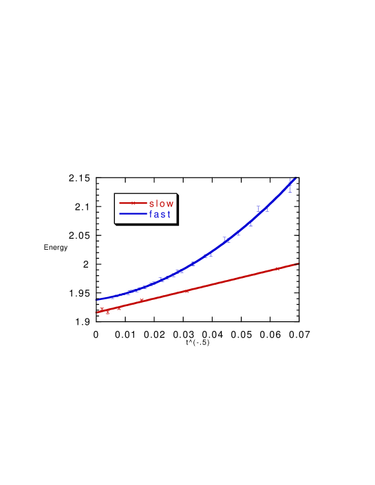
FIG. 8.: “fast” curve: energy as a function of $t^{-.5}$ where $t$ is the time spent at $\Gamma=1.8$ after a rapid quench; “slow” curve: energy reached at the end of the time spent at $\Gamma=1.8$, as a function of of $t^{-.5}$, where $t$ is the time spent at each temperature during the gradual quench process. We see that slower cooling yields lower energies. The continuation to $t^{-.5}\to 0$ corresponds to an infinitely slow cooling.

FIG. 9.: Evolution of the energy at $\Gamma=1.8$ ($T\approx 0.095$), in function of time, for various cooling rates; the horizontal lines correspond to $E_{F}$ and $E_{S}$. The lower curves correspond to slower coolings.

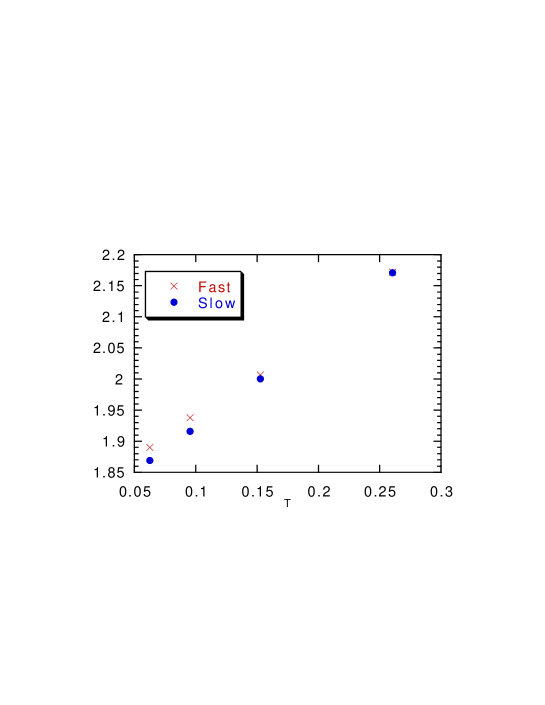
FIG. 10.: Extrapolations of the energies $E_{F}$ and $E_{S}$ at large times, i.e. asymptotic energies after a quench or after an infinitely slow cooling, for various temperatures.

VI Summary and Conclusions

In this paper we have investigated the behavior in temperature of the metastable states of long range spin-glasses with first order freezing transition. We have shown that the metastable states can be followed up and down in temperature, from the temperature where they are dominating the partition function. Going up in temperature, one finds some temperature where the states disappear, merging with some maxima. Going down in temperature, the state do never disappear, although in some range of $T^{\prime}$ multifurcation is found. We also studied the dynamics at temperature $T<T_{d}$, following a quench from equilibrium at temperature $T^{\prime}$. If $T^{\prime}>T_{d}$ we find no difference from the usual aging behavior [17] that follows a quench from infinite temperature. For $T^{\prime}<T_{d}$ we have found two possibilities. If $T>T_{rsb}(T^{\prime})$ the original valley has “deformed” but not bifurcated and the system is able to equilibrate inside it. In the complementary interval $T<T_{rsb}(T^{\prime})$ the landscape has changed drastically as the original valley has bifurcated. The system is then unable to thermalize and falls in an aging regime, while remaining confined in the vicinity of the initial data. Besides, this dynamical study shows that the aging after a slow quench (in the mean-field case, the case of thermalized initial conditions at $T^{\prime}$ can be thought of as a situation after an infinitely slow quench) allows to reach a situation where the behavior is qualitatively similar to the one after a rapid quench (i.e. aging corresponding to a slow touring of the phase space), but within a phase space region with lower energies. Therefore, at a given temperature $T$, the possibilities are not only of aging at a relatively high energy, after a sudden quench, or of equilibrium dynamics after an infinitely slow quench, but also of aging at intermediate energies, depending on the route from high temperature to $T$.

In the last section, we tried to emphasize the possible relevance of such mean-field scenarios for finite dimensions, where it has been advocated that metastable states may still exist, but with a finite lifetime: coming from a high temperature phase, the system may be able to find these states in a finite time, and the resulting aging behavior when decreasing the temperature could be a mixture of jumps between states and periods of wandering when states bifurcate.

Indeed, the numerical study of section V shows indications that, at least in the explored time window, for a soft sphere model of glass exhibiting aging, the dynamics is not dominated by activated processes. Depending on the cooling rate from the high temperature phase, various energies can be reached. Since the system is finite, it should however reach equilibrium in a finite time (the energy should reach the equilibrium energy, whatever may be the route to the final temperature) but, these simulations show that, even for a relatively small system, this finite time is very large, and therefore that mean-field conclusions can be of importance in the real world.

We consider the case when the primary minimum of the potential is in the RS region: $q_{0}=q_{1}\equiv q$. Then, for fixed $T^{\prime}$, we compute the value of $q_{12}$ and $q$ for this minimum, $q_{12}^{pr}$ and $q^{pr}$. The saddle point equations for $q_{0},\ q_{1},\ x$ reduce to

$$\beta^{2}f^{\prime}(q^{pr})=\frac{q^{pr}-{q_{12}^{pr}}^{2}}{(1-q^{pr})^{2}}\\$$ (43)

and the equation $\frac{\partial V}{\partial q_{12}}=0$ is

$$\beta\beta^{\prime}f^{\prime}(q_{12}^{pr})=\frac{q_{12}^{pr}}{1-q^{pr}}.$$ (44)

The value of the potential is

$$V_{primary}=-\beta^{\prime}f(q_{12}^{pr})+\frac{\beta}{2}f(q^{pr})-\frac{\beta}{2}(1-q^{pr})f^{\prime}(q^{pr})-\frac{1}{2\beta}{\rm ln}(1-q^{pr}).$$ (45)

The energy of the second replica, in this minimum, is

$$E_{primary}=\frac{\partial}{\partial\beta}(\beta V+\beta F(T))$$ (46)

which yields

$$E_{primary}=-\beta^{\prime}f(q_{12}^{pr})+\beta f(q^{pr})-\beta f(1)$$ (47)

On the other hand, we can write the TAP free energy as:

$$f_{TAP}(H,q,\beta)=H-\frac{1}{2\beta}{\rm ln}(1-q)-\frac{\beta}{2}(f(1)-f(q)-(1-q)f^{\prime}(q)),$$ (48)

where $q=\frac{1}{N}\sum_{i}m_{i}^{2}$, and $H$ is the value taken by the Hamiltonian $H(\{m_{i}\})$, so the energy of a TAP state ${m_{i}}$ is

$$E_{TAP}=\frac{\partial\beta f}{\partial\beta}=H-\beta(f(1)-f(q)-(1-q)f^{\prime}(q))$$ (49)

Then, taking

$$H_{pr}=E_{primary}+\beta(f(1)-f(q^{pr})-(1-q^{pr})f^{\prime}(q^{pr}),$$ (50)

we obtain immediately that

$$V_{primary}=f_{TAP}(H_{pr},q^{pr},\beta)-F_{RS}(T).$$ (51)

This means that $V_{primary}$ is the free energy cost of having the second replica in a TAP state with parameter $q^{pr}$ and energy $E_{primary}$ at inverse temperature $\beta$.

REFERENCES

- [1]
- [2] D.Sherrington, “Landscape Paradigms in Physics and Biology: Introduction and Overview” preprint cond-mat/9608088, to appear in Physica D, and references therein.
- [3] For a recent review see E. Marinari, G .Parisi, J .Ruiz-Lorenzo, Numerical Simulations of Spin Glass Systems, condmat/9701016, contribution to the volume: “Spin Glasses and Random Fields”, edited by P. Young.
- [4] D. J. Thouless, P. W. Anderson, and R. G. Palmer, Phil. Mag. 35, 593 (1977).
- [5] D. Thirumalai and T. R. Kirkpatrick, Phys. Rev. B 37 5342 (1988); T. R. Kirkpatrick and P. G. Wolynes, Phys. Rev. B 36 8552 (1987); D. Thirumalai and T. R. Kirkpatrick, Phys. Rev. B 38, 4881 (1988).
- [6] T. R. Kirkpatrick and D. Thirumalai, Phys. Rev. B 36, 5388 (1987).
- [7] T. R. Kirkpatrick, D. Thirumalai, and P. G. Wolynes, Phys. Rev. A 40, 1045 (1989).
- [8] G. Parisi, Il nuovo cimento 16, 939 (1994).
- [9] M. Mézard, G. Parisi, and M. A. Virasoro, Spin Glass Theory and Beyond, World Scientific, Singapore, 1987.
- [10] J. Kurchan, G. Parisi, and M. A. Virasoro, J. Phys. I France 3, 1819 (1993).
- [11] I. Kondor, J. Phys. A 22 L163 (1989); I. Kondor and A. Vegsö, J. Phys. A 26 L641 (1993).
- [12] S. Franz and M. Ney-Nifle, J. Phys. A 28 2499 (1995).
- [13] S. Franz and G. Parisi, J. Phys. I (France) 5, 1401 (1995).
- [14] R. Monasson, Phys. Rev. Lett. 75, 2847 (1995).
- [15] S. Franz and G. Parisi, Phase diagram of glassy systems in an external field, condmat 9701033.
- [16] A. Barrat, R. Burioni, and M. Mézard, J. Phys. A 29, L81 (1996).
- [17] L. F. Cugliandolo and J. Kurchan, Phys. Rev. Lett. 71, 173 (1993).
- [18] A. Cavagna, I. Giardina and G. Parisi, Structure of metastable states in spin glasses by means of a three replica potential, condmat 9611068.
- [19] A. Crisanti and H.-J. Sommers, J. Phys. I (France) 5, 805 (1995).
- [20] A. Barrat, The -spin spherical spin glass model, condmat 9701031.
- [21] H. Rieger, Phys. Rev. B 46, 14655 (1992).
- [22] S. Franz and M. Mézard, Physica A 210, 48 (1994).
- [23] A. Houghton, S. Jain, and A. P. Young, Phys. Rev. B 28, 290 (1983).
- [24] H. Horner, Z. Phys. B 66 175 (1987); A. Crisanti, H. Horner and H.J. Sommers, Z. Phys. B 92 257 (1993); E. De Santis, G. Parisi and F. Ritort, J. Phys. A: Math. Gen. 28 327 (1995).
- [25] B.Bernu, J.-P. Hansen, Y. Hitawari and G. Pastore, Phys. Rev. A36 4891 (1987).
- [26] J.-L. Barrat, J-N. Roux and J.-P. Hansen, Chem. Phys. 149, 197 (1990).
- [27] J.-P. Hansen and S. Yip, Trans. Theory and Stat. Phys. 24, 1149 (1995).
- [28] D. Lancaster and G. Parisi, A study of activated processes in soft sphere glass, cond-mat 9701045.
- [29] G. Parisi, Short time aging in binary glasses, cond-mat 9701015.
- [30] G. Parisi, On the mean field approach to glassy systems, cond-mat 9701034.
- [31] G. Parisi, Numerical indications for the existence of a thermodynamic transition in binary glasses, cond-mat 9701100.
- [32] S. Franz, E. Marinari and G. Parisi, J. Phys. A 28, 5437 (1995).
- [33] F. Ritort, Phys. Rev. Lett. 75, 1190 (1995); S. Franz and F. Ritort, Europhys. Lett. 31, 507 (1996); S. Franz and F. Ritort, J. Stat. Phys. 85, 131 (1996).
- [34] J. Kurchan and L. Laloux, J. Phys. A 29, 1929 (1996).