To appear in Chaos Solitons & Fractals
Special Issue on ”Chaos and Quantum Transport in Mesoscopic Cosmos”, editor: K. Nakamura (1997)

Diffraction in the semiclassical description of mesoscopic devices

G. VATTAY, J. CSERTI, G. PALLA and G. SZÁLKA

Institute for Solid State Physics, Eötvös University, Múzeum krt. 6-8, H-1088 Budapest, Hungary

Abstract -In pseudo integrable systems diffractive scattering caused by wedges and impurities can be described within the framework of Geometric Theory of Diffraction (GDT) in a way similar to the one used in the Periodic Orbit Theory of Diffraction (POTD). We derive formulas expressing the reflection and transition matrix elements for one and many diffractive points and apply it for impurity and wedge diffraction. Diffraction can cause backscattering in situations, where usual semiclassical backscattering is absent causing an erodation of ideal conductance steps. The length of diffractive periodic orbits and diffractive loops can be detected in the power spectrum of the reflection matrix elements. The tail of the power spectrum shows $\sim 1/l^{1/2}$ decay due to impurity scattering and $\sim 1/l^{3/2}$ decay due to wedge scattering. We think this is a universal sign of the presence of diffractive scattering in pseudo integrable waveguides.

In recent years, semiclassical methods became very popular in describing devices operating in the mesoscopic regime. There are two entirely different sets of theoretical tools which have been used in a wide range of applications. One of them is a WKB based short wavelength description [1, 2] where classical trajectories, chaos, regularity and analytic properties of the potential play a major role. The other is based on random matrix models or on averaging over random Gaussian potentials [3]. The first approach is designed to describe clean systems where the potential depends smoothly on coordinates and parameters, while the second assumes a system densely packed with impurities causing wild fluctuations of the potential on all length scales.

Fortunately, advances in manufacturing and material design reduced the average number of impurities exponentially since the eighties and this trend is expected to continue in the future. Accordingly, a realistic semiclassical theory should be capable to treat systems with low number of impurities and not only completely clean or completely dirty ones. Another demand is that human designed structures, straight sides and eventual wedges should be a natural part of the description. These systems, neither chaotic nor regular, form the intermediate class of pseudo integrable systems. In the present paper we will demonstrate that diffractive scattering caused by wedges and impurities can be described within the framework of Geometric Theory of Diffraction [4, 5, 6, 7, 8] (GDT) in a way similar to the one used in the Periodic Orbit Theory of Diffraction [9, 10, 11] (POTD). The POTD is an extension of Gutzwiller’s periodic orbit theory for non-smooth systems with diffractive scattering which has been used successfully during the last three years.

1 Examples of pseudo integrable mesoscopic devices

The simplest mesoscopic device is a two dimensional wave guide strip of electron gas, formed on a GaAs heterostructure [14], connecting two electron reservoirs (Fig. 1a).

Figure 1: Electron reservoirs (Ohmic contacts) connected trough strip waveguides. a, Ideal strip waveguide with parallel walls. b, Ideal strip waveguide with parallel walls and one pointlike impurity. c, Broken-strip waveguide.

This system can be considered also as a paradigm of a more sophisticated two or three dimensional clean quantum wire [15] made of other materials, for example carbon based structures with delocalized electrons. Here we will consider two slightly modified versions of this simple quantum wire, the quantum wire with one point like impurity (see Fig. 1b) [16], the broken-strip waveguide (see Fig. 1c) [17]. Our motivation in selecting these systems for investigations is that any long wire with straight sides, many wedges and impurities can be built up as a sequence of these building blocks. For simplicity, the walls of the wave guides are assumed to be completely hard and the wave function vanishes on them. The potential is assumed to be zero inside the waveguide.

2 The Landauer Formula

The conductance of the non-degenerate electron gas in a waveguide considered here is given by the Landauer formula [18, 19]. According to this theory, incoming and outgoing wave functions in the leads far from impurities or wedges can be decomposed into incoming and outgoing quantum modes

$$\psi_{n}(x,y) = \Phi_{n}(y)e^{ik_{n}x},$$

$$\Phi_{n}(y) = \sqrt{\frac{2}{W}}\sin(\pi ny/W),$$ (1)

where $k_{n}=\sqrt{2mE_{F}-(\hbar\pi n/W)^{2}}/\hbar$ is the wave number of the propagating planewave, $W$ is the width of the lead and $E_{F}$ is the Fermi energy. If the Fermi energy is less than $E_{n}=\frac{1}{2m}(\hbar\pi n/W)^{2}$ the wavenumber $k_{n}$ becomes imaginary and the $n^{th}$ channel becomes closed preventing wave propagation.

The Landauer formula for the conductance $G(E_{F})$ at Fermi energy $E_{F}$ is then

$$G(E_{F})=\frac{2e^{2}}{h}\sum_{m,n}|t_{mn}|^{2},$$ (2)

where $t_{nm}$ is the transition probability amplitude from the incoming cannel $n$ on the entrance side to the outgoing channel $m$ on the exit side. In case of infinitely long leads summation goes for open channels of both sides only. The transition probability is given by the projection of the Green function over the transverse wave functions $\Phi_{n}(y)$ on the entrance lead for the incoming modes and $\Phi_{m}^{\prime}(y^{\prime})$ on the exit lead for outgoing modes

$$t_{nm}=2i(k_{n}k_{m}^{\prime})^{1/2}\int dydy^{\prime}\Phi_{n}(y)G^{+}(x,y|x^{\prime},y^{\prime})\Phi_{m}^{\prime}(y^{\prime}),$$ (3)

and $x$ and $x^{\prime}$ lie anywhere on the entrance side and exit side, respectively (See Fig. 1a-c). (From here on we will use units such $\hbar=2m=1$.) Reflection between two modes $n$ and $m$ on the same side is given by

$$r_{nm}=\delta_{nm}-2i(k_{n}k_{m})^{1/2}\int dydy^{\prime}\Phi_{n}(y)G^{+}(x,y|x,y^{\prime})\Phi_{m}(y^{\prime}),$$ (4)

where $x$ lies anywhere on the entrance side. For open channels $n$ of the entrance side the transmission and reflection amplitudes fulfill the sum rules

$$\sum_{m}|t_{nm}|^{2}+\sum_{m^{\prime}}|r_{nm^{\prime}}|^{2}=1,$$ (5)

where the two summation goes for channels $m$ on the exit side and $m^{\prime}$ on the entrance side. These are the consequences of the probability and current conservation. Thanks to these relations, in infinitely long wave guides, the conductance can be expressed with the reflection coefficients

$$G(E_{F})=\frac{2e^{2}}{h}\left(N-\sum_{m,n}|r_{nm}|^{2}\right),$$ (6)

where $N$ is the number of open channels on the exit side.

The direct connection between the Green function and the conductance makes it possible to develop a semiclassical approximation for the conductance based on the semiclassical Van Vleck - Gutzwiller type expressions for the Green function. Next, we summarize the main tools of the semiclassical description.

3 The semiclassical Green function

The Schrödinger equation in the waveguides leads to the Helmholtz equation

$$(\Delta+k^{2})\psi(q)=0,$$ (7)

where the notation $k=\sqrt{2mE/\hbar^{2}}$ has been introduced. The wavefunction vanishes on the boundary as we discussed above. The energy domain Green function of the Helmholtz equation is defined by

$$(\Delta+k^{2})G(q,q^{\prime},E)=\delta(q-q^{\prime}),$$ (8)

and $G(q,q^{\prime},E)$ should vanish on the boundary of the waveguide too. In absence of walls in two dimensions the outgoing Green function is given by

$$G^{+}(q,q^{\prime},E)=-\frac{i}{4}H^{(1)}_{0}(kd(q,q^{\prime})),$$ (9)

where $H^{(1)}_{0}(x)$ is the Hankel function of first kind and $d(q,q^{\prime})$ is the distance between $q$ and $q^{\prime}$. The semiclassical ($\hbar\rightarrow 0$) approximation of this free space Green function can be recovered from the asymptotic form of the Hankel function for large argument

$$G^{+}(q,q^{\prime},E)=\frac{1}{\sqrt{8\pi kd(q,q^{\prime})}}e^{ikd(q,q^{\prime})-i3\pi/4}.$$ (10)

A very useful optical interpretation of this formula can be given by tracing the ray connecting $q$ with $q^{\prime}$. The phase of the Green function is the classical action calculated along the ray

$$\int_{q}^{q^{\prime}}p(q^{\prime\prime})dq^{\prime\prime}=kd(q,q^{\prime}).$$

The amplitude of the Green function is the square root of the intensity

$$I(r)=\frac{1}{8\pi kr}$$ (11)

of a radiating point source where the distance from the source is $r=d(q,q^{\prime})$. The phase factor $e^{-i3\pi/4}$ is the Maslov index of the caustics singularity standing right in the source point $q$.

In the presence of walls, in general, more than one ray from $q$ can reach the point in $q^{\prime}$. Then the semiclassical Green function is a sum for the raywise Green functions calculated along the rays

$$G(q,q^{\prime},E)=\sum_{\forall r\\ q\rightarrow q^{\prime}}G_{0}^{r}(q,q^{\prime},E).$$ (12)

The phase of the Green functions $G_{0}^{r}$ is given by the classical action plus the Maslov index including the caustics in the source point. The amplitude is the square root of the intensity observable in $q^{\prime}$ coming form $q$ along the ray. In the endpoint we will see the mirror image of the source trough perfect mirrors given by the walls. The intensity in this case is given by the same formula (11), but now the effective radius of the spherical wave coming from $q$ should be used. If the walls are non curved this radius is simply the distance $d_{r}(q,q^{\prime})$ of $q$ and $q^{\prime}$ along the ray. In this case the Green function is given by

$$G_{0}^{r}(q,q^{\prime},E)=\frac{(-1)^{n_{r}}}{\sqrt{8\pi kd_{r}(q,q^{\prime})}}e^{ikd_{r}(q,q^{\prime})-i3\pi/4},$$ (13)

where $n_{r}$ is the number of bounces along the ray. For the semiclassical expression of the Green function in presence of curved walls the effective radius is given [11] by the product of the distance between the source and the first bounce point $l_{1}$ times the stretching factor $\Lambda$

$$r_{eff}=l_{1}\Lambda.$$ (14)

The stretching factor is the analog of the optical magnification factor of curved mirrors. It can be calculated as

$$\Lambda=\prod_{i=1}^{n-1}(1+\kappa_{i}^{+}l_{i}),$$ (15)

where $l_{i}$ is the length of the free flight between the $i^{th}$ and the $(i+1)^{th}$ bounces and $\kappa$ is the Bunimovich-Sinai curvature. The Bunimovich-Sinai curvature is defined recursively

$$\kappa_{i}^{+} = \kappa_{i}^{-}+2/r_{i}\cos(\phi_{i}),$$

$$\kappa_{i+1}^{-} = \kappa_{i}^{+}/(1+\kappa_{i}^{+}l_{i}),$$ (16)

where $r_{i}$ is the radius of curvature of the wall in the point of bounce and $\phi_{i}$ is the angle of incidence. The initial condition of the recursion is $\kappa_{1}^{-}=1/l_{1}$, which is the Bunimovich-Sinai curvature of the wavefront arriving at the first bounce point from the source. The Green function reads as

$$G_{0}^{r}(q,q^{\prime},E)=\frac{(-1)^{n_{r}}}{\sqrt{8\pi kl_{1}\Lambda_{r}}}e^{ikd_{r}(q,q^{\prime})-i3\pi/4}.$$ (17)

In the special case of non-curved walls the stretching factor (optical magnification) is $\Lambda=d_{r}(q,q^{\prime})/l_{1}$ yielding the expression (13).

4 Geometric Theory of Diffraction

The semiclassical approximation works well when changes of the potential are on a length scale much larger than the wavelength of the electron $1/k$ [20]. Even if the manufactured system in large satisfies this condition, there are isolated points such as corners or impurities where this cannot be the case. These points require special treatment [9, 12, 13]. They break the smooth wavefronts of the semiclassical wave propagation and create diffracted waves coiling out from them. Such diffractive points can be considered as new wave sources whose strength is proportional with the strength of the incident wave. Their contribution of such a specific ray to the Green function is given by

$$G_{d}(q,q^{\prime},k)=G_{0}(q,q_{0},k){\cal D}(\phi_{in},\phi_{out},k)G_{0}(q_{0},q^{\prime},k),$$ (18)

where $G_{0}(q,q_{0},k)$ is the Green function calculated along the ray connecting the source point $x$ and the diffractive point $q_{0}$, ${\cal D}(\phi^{r}_{in},\phi^{r}_{out})$ is the diffraction constant which can depend on the incoming and the outgoing angle of the ray and the energy. $G_{0}(q_{0},q^{\prime},k)$ is the Green function calculated from the source to the point of observation $q^{\prime}$. If there is more than one ray connecting $q$ with $q_{0}$ and $q_{0}$ with $q^{\prime}$ then each ray configuration from $q$ to $q^{\prime}$ will contribute to the Green function according to (18).

The diffraction constant can be determined for different geometric situations. For wedge diffraction

$${\cal D}(\phi_{in},\phi_{out})=\frac{\sin(\pi/n)}{n}\left[\frac{1}{\cos(\pi/n)-\cos((\phi_{in}-\phi_{out})/n)}-\frac{1}{\cos(\pi/n)-\cos((\pi+\phi_{in}+\phi_{out})/n)}\right],$$ (19)

where $(2-n)\pi$ is the opening angle of the wedge. For details we refer to Ref. [5, 11, 12]. For diffraction on impurities the $s$ wave scattering is dominant and the diffraction constant ${\cal D}$ is isotropic, depending only on the energy. Typical example is a $\delta$-shaped potential with scattering strength ${\cal D}$.

5 Semiclassical transmission and reflection

Semiclassically the transmission (3) and reflection (4) matrix elements are calculated by replacing the Green function in (3) and (4) with the semiclassical expressions (17) or (13). The wave functions $\Phi_{n}(y)$ and $\Phi_{m}^{\prime}(y^{\prime})$ can be decomposed to exponentials

$$\Phi_{n}(y) = \frac{1}{2i}\sqrt{\frac{2}{W}}\left(e^{in\pi y/W}-e^{-in\pi y/W}\right),$$

$$\Phi_{m}(y^{\prime}) = \frac{1}{2i}\sqrt{\frac{2}{W^{\prime}}}\left(e^{im\pi y^{\prime}/W^{\prime}}-e^{-im\pi y^{\prime}/W^{\prime}}\right).$$ (20)

The transmission and reflection matrix elements are then sums of four subintegrals

$$r_{nm} = r_{nm}^{++}+r_{nm}^{+-}+r_{nm}^{-+}+r_{nm}^{--},$$

$$t_{nm} = t_{nm}^{++}+t_{nm}^{+-}+t_{nm}^{-+}+t_{nm}^{--},$$ (21)

where

$$t_{nm}^{\pm\pm} = i(k_{n}k_{m}^{\prime})^{1/2}\frac{1}{\sqrt{WW^{\prime}}}\int dydy^{\prime}e^{\pm in\pi y/W\pm im\pi y^{\prime}/W^{\prime}-i\nu\pi/2}G^{+}(x,y|x^{\prime},y^{\prime}),$$

$$r_{nm}^{\pm\pm} = \frac{\delta_{nm}}{4}-i(k_{n}k_{m})^{1/2}\frac{1}{W}\int dydy^{\prime}e^{\pm in\pi y/W\pm im\pi y^{\prime}/W-i\nu\pi/2}G^{+}(x,y|x,y^{\prime}),$$ (22)

where $\nu=\pm 1\pm 1$. By using (17) or (13) in semiclassical approximation one can calculate these integrals with saddle point approximation. The saddle point conditions for various $t_{nm}^{\pm\pm}$-s are

$$k\partial_{y}d_{r}(x,y|x^{\prime},y^{\prime}) = \mp\pi n/W\qquad\mbox{and}$$

$$k\partial_{y^{\prime}}d_{r}(x,y|x^{\prime},y^{\prime}) = \mp\pi m/W^{\prime},$$ (23)

and for $r_{nm}^{\pm\pm}$-s are

$$k\partial_{y}d_{r}(x,y|x,y^{\prime}) = \mp\pi n/W\qquad\mbox{and}$$

$$k\partial_{y^{\prime}}d_{r}(x,y|x,y^{\prime}) = \mp\pi m/W.$$ (24)

If we introduce the initial $\phi_{in}$ and final $\phi_{fin}$ angle of the rays with respect to the direction of the leads these conditions are equivalent with selecting rays whose initial angle is determined by

$$\sin(\phi_{in})=\mp\frac{n\pi}{kW}$$ (25)

and their final angle is

$$\sin(\phi_{fin}) = \mp\frac{m\pi}{kW^{\prime}}\qquad\mbox{for $t_{nm}$},$$

$$\sin(\phi_{fin}) = \mp\frac{m\pi}{kW}\qquad\mbox{for $r_{nm}$},$$ (26)

respectively.

For irregularly shaped wave guides one can in general find rays starting and ending with given initial and final angles. We can call such systems ”chaotic”. In wave guides formed by regularly shaped walls it is possible that in the bouncing process a components of the momentum is conserved in addition to the energy conservation. In these systems only one of the saddle point conditions can be satisfied. We can call them ”integrable”. One example is the waveguide on Fig. 1a. There are systems, where chaotic and integrable behaviour coexist. For certain initial angle one can find rays to any final angle, while for other initial conditions not. These systems are ”mixed”. The conductance of chaotic, integrable and mixed systems are relatively well understood.

The simple, typically human designed systems of Fig. 1b and Fig. 1c do not belong to any of these categories. We may call them ”pseudo integrable” systems. These systems are not chaotic, since there exist is no ray in general connecting a given initial and a final angle. An initial angle allows only a finite number of possible final angles. So, they are more like integrable systems in this respect. However, when we take into account the diffractive points, rays can leave them in any direction. So, we can always find diffractive rays connecting any initial angle with any final one. In this respect, these systems are more chaotic like.

In the wave guides on Fig. 1b and 1c starting from the left with a given initial angle and bouncing on the walls, the electron can end up on the right with a definite final angle. Return to the left is impossible. Except for a classically ”measure zero” fraction of rays hitting the impurity or the wedge. The contribution of these rays to the transmission and to the reflection can be computed by substituting the diffractive part of the Green function (18) into (22). The length of the ray connecting $(x,y)$ with $(x^{\prime},y^{\prime})$ or $(x,y^{\prime})$ via the diffractive point $(x_{0},y_{0})$ is

$$d(x,y|x^{\prime},y^{\prime}) = d(x,y|x_{0},y_{0})+d(x_{0},y_{0}|x^{\prime},y^{\prime}),$$

$$d(x,y|x,y^{\prime}) = d(x,y|x_{0},y_{0})+d(x_{0},y_{0}|x,y^{\prime}).$$ (27)

Since the position of the diffractive point $(x_{0},y_{0})$ is fixed, the saddle point conditions for the initial and final segments decouple for $t_{nm}^{\pm\pm}$-s

$$k\partial_{y}d(x,y|x_{0},y_{0}) = \mp\pi n/W\qquad\mbox{and}$$

$$k\partial_{y^{\prime}}d(x_{0},y_{0}|x^{\prime},y^{\prime}) = \mp\pi m/W^{\prime},$$ (28)

and for the $r_{nm}^{\pm\pm}$-s

$$k\partial_{y}d(x,y|x_{0},y_{0}) = \mp\pi n/W\qquad\mbox{and}$$

$$k\partial_{y^{\prime}}d(x_{0},y_{0}|x,y^{\prime}) = \mp\pi m/W.$$ (29)

The saddle point integrals

$$t_{nm}^{\pm\pm} = \frac{i(k_{n}k_{m}^{\prime})^{1/2}}{\sqrt{WW^{\prime}}}\int dydy^{\prime}e^{\pm in\pi y/W\pm im\pi y^{\prime}/W^{\prime}-i\nu\pi/2}G_{0}(x,y|x_{0},y_{0}){\cal D}(\phi_{in},\phi_{out})G_{0}(x_{0},y_{0}|x^{\prime},y^{\prime}),$$

$$r_{nm}^{\pm\pm} = -\frac{i(k_{n}k_{m})^{1/2}}{W}\int dydy^{\prime}e^{\pm in\pi y/W\pm im\pi y^{\prime}/W-i\nu\pi/2}G_{0}(x,y|x_{0},y_{0}){\cal D}(\phi_{in},\phi_{out})G_{0}(x_{0},y_{0}|x,y^{\prime})$$ (30)

then can be carried out separately. The Kronecker delta disappears, as usual [19, 20], due to the trivial direct rays from $y$ to $y^{\prime}$. Assuming straight walls we get

$$t_{nm}^{\pm\pm} = -i{\cal D}(\phi_{in},\phi_{out})\frac{(-1)^{n_{r}}}{4\sqrt{WW^{\prime}k_{n}k_{m}^{\prime}}}e^{ik(d(x,\bar{y}|x_{0},y_{0})+d(x_{0},y_{0}|x^{\prime},\bar{y}^{\prime}))\pm in\pi\bar{y}/W\pm im\pi\bar{y}^{\prime}/W^{\prime}-i\nu\pi/2},$$

$$r_{nm}^{\pm\pm} = +i{\cal D}(\phi_{in},\phi_{out})\frac{(-1)^{n_{r}}}{4W\sqrt{k_{n}k_{m}}}e^{ik(d(x,\bar{y}|x_{0},y_{0})+d(x_{0},y_{0}|x,\bar{y}^{\prime}))\pm in\pi\bar{y}/W\pm im\pi\bar{y}^{\prime}/W-i\nu\pi/2},$$ (31)

where $n_{r}$ is the total number of bounces on the straight wall and $\bar{y}$ and $\bar{y}^{\prime}$ are the solutions for the saddle point conditions (28) and (29). The $\pm$ signs in $\bar{y}_{\pm}$ and $\bar{y}_{\pm}^{\prime}$ have been suppressed for brevity.

A ray with only one diffractive point is the most elementary possibility for diffraction. More complicated diffractive rays are those, which return to the diffractive point several times. These events are described by the following Green function

$$G_{d}(x,y|x^{\prime},y^{\prime})=G_{0}(x,y|x_{0},y_{0})G_{0}(x_{0},y_{0}|x^{\prime},y^{\prime})\left({\cal D}(\phi_{in},\phi_{out})+\sum_{r}{\cal D}(\phi_{in},\phi_{r})G_{0}^{r}(\phi_{r},\phi_{r}^{\prime}){\cal D}(\phi_{r}^{\prime},\phi_{out})\right),$$ (32)

where $\phi_{in}$ and $\phi_{out}$ denote the angles under which the incoming and outgoing rays reach first and leave finally the diffractive point, $\phi_{r}$ and $\phi_{r}^{\prime}$ stand for starting and ending angles of ray loops starting and ending in the diffractive points and $G_{0}^{r}(\phi_{r},\phi_{r}^{\prime})$ denotes the Green function computed along this ray loop. The expression in the bracket can be considered as an effective diffraction constant, renormalized by the interaction with the environment. The closed ray loops starting and ending in a diffractive point were introduced in Ref.[9] first and are called diffractive periodic orbits. The summation for $r$ is a summation for all the possible diffractive periodic orbits starting and ending in the diffractive point

$$\tilde{{\cal D}}(\phi_{in},\phi_{out})={\cal D}(\phi_{in},\phi_{out})+\sum_{p}A_{p}e^{ikd_{p}},$$ (33)

where $d_{p}$ is the length of the diffractive periodic orbit and $A_{p}=|{\cal D}(\phi_{in},\phi_{p},k)G_{r}(\phi_{p},\phi_{p}^{\prime}){\cal D}(\phi_{p}^{\prime},\phi_{out})|$. The transmission and reflection matrix elements then can be written in terms of the renormalized diffraction constants

$$t_{nm}^{\pm\pm} = -i\tilde{{\cal D}}(\phi_{in},\phi_{out})\frac{(-1)^{n_{r}}}{4\sqrt{WW^{\prime}k_{n}k_{m}^{\prime}}}e^{ik(d(x,\bar{y}|x_{0},y_{0})+d(x_{0},y_{0}|x^{\prime},\bar{y}^{\prime}))\pm in\pi\bar{y}/W\pm im\pi\bar{y}^{\prime}/W^{\prime}-i\nu\pi/2},$$

$$r_{nm}^{\pm\pm} = +i\tilde{{\cal D}}(\phi_{in},\phi_{out})\frac{(-1)^{n_{r}}}{4W\sqrt{k_{n}k_{m}}}e^{ik(d(x,\bar{y}|x_{0},y_{0})+d(x_{0},y_{0}|x,\bar{y}^{\prime}))\pm in\pi\bar{y}/W\pm im\pi\bar{y}^{\prime}/W-i\nu\pi/2}.$$ (34)

The expression derived here is the main result of the paper and expresses the diffractive part of the transmission and reflection matrix elements in terms of diffractive periodic orbits and the rays reaching and leaving the impurity.

In case of more than one diffractive points $q_{0},...,q_{k}$, one can imagine more complicated situations. The ray from $y$ can reach $q_{l}$ first, then jumps to $q_{s}$ and goes to $y^{\prime}$. Beyond the direct ray between $l$ and $s$, there are rays which start in $l$ and reach $s$ in different ways, possibly trough diffraction on other diffractive points or trough bouncing on the walls or trough some combination of these. These type of processes are described by the Green function

$$G_{d}(x,y|x^{\prime},y^{\prime})=\sum_{l,s}G_{0}(x,y|x_{l},y_{l})G_{0}(x_{s},y_{s}|x^{\prime},y^{\prime})\left(\sum_{r}{\cal D}(\phi_{y\rightarrow l},\phi_{r})G_{0}^{r}(\phi_{r},\phi_{r}^{\prime}){\cal D}(\phi_{r}^{\prime},\phi_{s\rightarrow y^{\prime}})\right),$$ (35)

where $G_{r}(\phi_{r},\phi_{r}^{\prime})$ is the Green function computed along the ray leaving $l$ at angle $\phi$ and reaching $s$ at angle $\phi^{\prime}$. We can introduce the notations

$$\tilde{{\cal D}}_{ls}(\phi_{y\rightarrow l},\phi_{s\rightarrow y^{\prime}},k)=\sum_{r}{\cal D}(\phi_{y\rightarrow l},\phi_{r})G_{0}^{r}(\phi_{r},\phi_{r}^{\prime}){\cal D}(\phi_{r}^{\prime},\phi_{s\rightarrow y^{\prime}}),$$ (36)

where the diagonal terms $\tilde{{\cal D}}_{ll}(\phi_{y\rightarrow l},\phi_{s\rightarrow y^{\prime}},k)$ are defined as the renormalized diffraction constants defined in (33). Finally, we can compute the transmission and reflection matrix elements as before and get

$$t_{nm}^{\pm\pm} = -i\sum_{ls}\tilde{{\cal D}}_{ls}(\phi_{in,l},\phi_{out,s},k)\frac{(-1)^{n_{ls}}}{4\sqrt{WW^{\prime}k_{n}k_{m}^{\prime}}}e^{ik(d(x,\bar{y}|x_{l},y_{l})+d(x_{s},y_{s}|x^{\prime},\bar{y}^{\prime}))\pm in\pi\bar{y}/W\pm im\pi\bar{y}^{\prime}/W^{\prime}-i\nu\pi/2},$$

$$r_{nm}^{\pm\pm} = +i\sum_{ls}\tilde{{\cal D}}_{ls}(\phi_{in,l},\phi_{out,s})\frac{(-1)^{n_{ls}}}{4W\sqrt{k_{n}k_{m}}}e^{ik(d(x,\bar{y}|x_{l},y_{l})+d(x_{s},y_{s}|x^{\prime},\bar{y}^{\prime}))\pm in\pi\bar{y}/W\pm im\pi\bar{y}^{\prime}/W-i\nu\pi/2}.$$ (37)

This is the most general expression, within the framework of the GDT, for the transmission and reflection matrix elements.

Next, we are going to apply the theory developed here for the examples announced in the introduction and show which are the consequences of diffractive contributions for the conductance of these systems.

6 Erosion of conductance steps

We have calculated the conductance of an infinitely long waveguide with a point like impurity in its center and the broken-strip waveguide (see Fig. 2).

Figure 2: Conductance as a function of the Fermi wavelength in units of $\frac{\pi}{W}$ a, For the infinite strip with impurity (${\cal D}=1$). b, For the broken-strip waveguide. The angle of the strips measured from the line connecting the two wedges were $\pi/6$ and $\pi/2$.

The details of the calculation will be published elsewhere[22, 21]. The geometry in both cases is such, that a classical electron starting from the left of the device cannot return back via classical bounces on the walls[23]. The usual semiclassical theory, in the absence of returning rays, predicts no reflection for these systems and the semiclassical reflection matrix elements $r_{nm}$ all vanish. According to (6) the conductance of such systems should coincide with that of an ideal straight waveguide $G(E_{F})=\frac{2e^{2}}{h}N$. As we can see on Fig. 2, this is not the case. The difference between the sharp ideal staircase and the actual conductance is the consequence of the non-vanishing reflection. In case of the pointlike impurity the reflection can be determined exactly and various terms can be interpreted from a diffractive point of view. The exact reflection matrix elements for an impurity in an infinite straight waveguide are

$$r_{nm}=-\Phi_{n}(y_{0})\Phi_{m}(y_{0})\frac{1}{2i\sqrt{k_{n}k_{m}}}e^{ik_{n}|x-x_{0}|+ik_{m}|x-x_{0}|}\frac{{\cal D}}{1-{\cal D}\tilde{G}_{E}(x_{0},y_{0}|x_{0},y_{0})},$$ (38)

where the exact Green function of the empty guide

$$G_{E}(x,y|x^{\prime},y^{\prime})=\sum_{n}\frac{\Phi_{n}(y)\Phi_{n}(y^{\prime})}{2ik_{n}}e^{ik_{n}|x-x^{\prime}|}$$ (39)

has been evaluated on the impurity and the singularity has been removed

$$\tilde{G}_{E}(x_{0},y_{0}|x_{0},y_{0})=\lim_{\epsilon\rightarrow 0}\left(G_{E}(x_{0}+\epsilon,y_{0}|x_{0},y_{0})+\frac{1}{4}Y_{0}(k\epsilon)\right),$$ (40)

where $Y_{0}(x)$ is the Neumann function. By using (20) we can determine the exact $r^{\pm\pm}_{nm}$ elements:

$$r_{nm}^{\pm\pm}=e^{\pm iny_{0}/W\pm imy_{0}/W}\frac{i}{4W\sqrt{k_{n}k_{m}}}e^{ik_{n}|x-x_{0}|+ik_{m}|x-x_{0}|-i\nu\pi/2}\frac{{\cal D}}{1-{\cal D}\tilde{G}_{E}(x_{0},y_{0}|x_{0},y_{0})}.$$ (41)

These terms can be interpreted as contributions from various rays reaching the impurity. For example a ray starting in $x,\bar{y}$ under angle $\sin(\phi_{in})=n\pi/Wk$ will reach $x_{0},y_{0}$ by flying a distance $|x-x_{0}|$ in horizontal direction and $|y_{0}-\bar{y}|+rW$ in the vertical direction, where $r$ is the number of bounces during the flight, the total length of the ray is

$$d(x,\bar{y}|x_{0},y_{0})=(|x-x_{0}|^{2}+(|y_{0}-\bar{y}|+rW)^{2})^{1/2},$$

and

$$\cos(\phi_{in})=|x-x_{0}|/d(x,\bar{y}|x_{0},y_{0}),\;\;\sin(\phi_{in})=(|y_{0}-\bar{y}|+rW)/d(x,\bar{y}|x_{0},y_{0}).$$

Using the relation $k_{n}=k\cos(\phi_{in})$ the full exponential can be written as

$$k_{n}|x-x_{0}|+n\pi y_{0}/W=kd\cos^{2}(\phi_{in})+k\sin(\phi_{in})(d\sin(\phi_{in})-rW+\bar{y})=kd-rn\pi+n\pi\bar{y}/W.$$

Replacing the phase terms in (41) with this and analogous expression for the other ray (see Fig. 3a) we recover (34) exactly with renormalized diffraction constant

$$\tilde{{\cal D}}=\frac{{\cal D}}{1-{\cal D}\tilde{G}_{E}(x_{0},y_{0}|x_{0},y_{0})}.$$ (42)

It is very reassuring to see diffraction theory reproducing the exact result in this case.

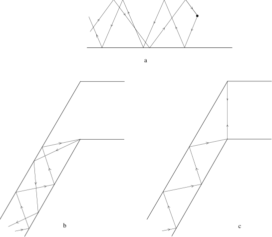
Figure 3: Typical diffractive rays. a, Primary rays reaching and leaving the diffractive point created by the pointlike impurity. b Primary rays reaching and leaving the diffractive point in the wedge. c Primary ray and the ray bouncing forth and back between the diffractive points.

The regularized Green function can be written semiclassically as a sum for all trajectories starting on and returning to the singularity[24]

$$\tilde{G}_{E}(q_{0},q_{0})\approx\sum_{r\;q_{0}\rightarrow q_{0}}\frac{(-1)^{n_{r}}}{\sqrt{8\pi kd_{r}}}e^{ikd_{r}-i3\pi/4}.$$ (43)

Accordingly the renormalized diffraction constant

$$\tilde{{\cal D}}={\cal D}+{\cal D}^{2}\tilde{G}_{0}(x_{0},y_{0}|x_{0},y_{0})+{\cal D}^{3}\tilde{G}_{0}^{2}(x_{0},y_{0}|x_{0},y_{0})+...$$ (44)

can be viewed as a sum for all returning rays having one, two, … etc. diffractions on their way.

It is very enlighting to study on this simple model how diffraction erodes the conductance steps close to Fermi wavelengths where new channels are opened $k\rightarrow\pi n/W$ ($k_{n}\rightarrow 0)$. Around these Fermi wavelengths the regularized Green function is dominated by a single term

$$\tilde{G}_{0}(q_{0},q_{0})\approx\frac{\Phi_{n}(y_{0})\Phi_{n}(y_{0})}{2ik_{n}}.$$ (45)

The squares of the reflection matrix elements can be approximated by

$$|r_{nm}|^{2}=\frac{k_{n}}{k_{m}}\frac{|\Phi_{m}(y_{0})|^{2}}{|\Phi_{n}(y_{0})|^{2}}\frac{1}{1+\frac{4k_{n}^{2}}{{\cal D}^{2}|\Phi_{n}(y_{0})|^{4}}}.$$ (46)

The nondiagonal reflection coefficients are small and vanish for $k_{n}\rightarrow+0$, while the diagonal is a Lorentzian of width $\Delta_{n}={\cal D}|\Phi_{n}(y_{0})|^{2}/2$

$$|r_{nn}|^{2}=\frac{1}{1+(k_{n}/\Delta_{n})^{2}},\qquad k_{n}>0.$$ (47)

Accordingly, the conductance steps have an eroded shape

$$G=\frac{2e^{2}}{h}(N-|r_{nn}|^{2})=\frac{2e^{2}}{h}\left(N-1+\frac{(k_{n}/\Delta_{n})^{2}}{1+(k_{n}/\Delta_{n})^{2}}\right).$$ (48)

We can see, that the average width of the erosion of the conductance steps is a primarily information about the level of diffraction in a waveguide (see Fig. 2a).

The diffraction theory is not exact for the broken-strip waveguide, but the conductance shows qualitatively the same behaviour (Fig. 2b). The main difference is that the diffraction constants here depends on the angle and reflection matrix elements are more complicated. The primary diffractive rays reaching and leaving the wedge are depicted on Fig. 3b. For $k$ just above $\pi n/W$ the initial angle is close to $\phi_{in}\approx\pi/2$ e.g. the electron is bouncing almost perpendicularly on the walls of the guide and cannot reach the upper wedge via bounces. On Fig. 3c a ray reaching the lower wedge by bounces and then going to the other wedge by diffraction is shown. When $k$ gets a bit larger, the initial angle decreases and rays reaching the other wedge directly should be considered. The sudden appearance of the new ray causes an abrupt change in $r_{11}$ at $k=1.5$ on Fig. 4.

For larger $k>>\pi n/W$ Fermi wavelengths the reflection matrix elements decrease rapidly and show oscillations small amplitude oscillations dominated by the oscillations coming from individual diffractive orbits (see Fig. 4).

Figure 4: The reflection matrix element $r_{11}$ as a function of the Fermi wavelength in units of $\frac{\pi}{W}$ a, for the strip waveguide with impurity b, for the broken-strip waveguide. (Re $r_{11}(k)$, Im $r_{11}(k)$ are denoted by solid and dashed lines, respectively.)

7 Diffractive periods in the power spectrum

For $k>>\pi n/W$ both $k_{n}$ and $k_{m}$ can be approximated with $k$. The primary diffractive rays are almost parallel with the walls of the guide $\phi\approx 0$. Since the Green functions of the rays have a prefactor proportional with $1/\sqrt{k}$, multiple diffractions are largely suppressed. The reflection matrix elements can be well approximated in leading $1/k$ order by keeping rays with one and two diffractive points only. Rays going trough two impurities while traversing the system are the most trivial examples. The first non-trivial contributions come from rays reaching a diffractive point and leaving it after making a loop.

In case of the point impurity this means that we keep terms proportional with the first and second power of the diffraction constant only:

$$r_{nm}\approx-\Phi_{n}(y_{0})\Phi_{m}(y_{0})\frac{1}{2ik}e^{ik_{n}|x-x_{0}|+ik_{m}|x-x_{0}|}\left({\cal D}+{\cal D}^{2}\tilde{G}_{E}(x_{0},y_{0}|x_{0},y_{0})\right).$$ (49)

The regularized Green function can be written as a sum for rays starting and ending on the impurity yielding

$$r_{nm}\approx-\Phi_{n}(y_{0})\Phi_{m}(y_{0})\frac{1}{2ik}e^{i2k|x-x_{0}|}\left({\cal D}+{\cal D}^{2}\sum_{q_{0}\rightarrow q_{0}}\frac{(-1)^{n_{r}}}{\sqrt{8\pi kd_{r}}}e^{ikd_{r}(q_{0},q_{0})-i3\pi/4}\right).$$ (50)

Beyond the trivial phase factor $e^{i2k|x-x_{0}|}$ coming from the ray reaching and leaving the impurity, the most important oscillations are caused by rays making a single loop starting and ending on the impurity. The length of these orbits can be calculated and can be grouped in three subcategories

$$d_{r} = 2y_{0}+2Wr,$$

$$d_{r} = 2(W-y_{0})+2Wr,$$ (51)

$$d_{r} = 2Wr,$$

where $r=0,1,2,...$. The amplitude of the oscillations is proportional with $1/\sqrt{d_{r}}\sim 1/\sqrt{r}$.

In the broken-strip waveguide the situation is somewhat more complicated. Loops starting and ending on the wedges can do it typically by making additional diffraction on the other wedge as shown on Fig. 2. But this diffraction process is somewhere in between a usual perpendicular bounce back from a wall and a diffraction in the corner. Therefore, the contributions of these orbits is not suppressed after one bounce. To see how the amplitude of these orbits decreases, we Fourier transformed the large $k$ tail of the reflection matrix element $r_{11}$ and calculated the power spectra

$$\tilde{r}_{11}(l)=\left|\int_{k_{0}}^{\infty}dkr_{11}(k)e^{-ikl}\right|,$$ (52)

where $k_{0}\approx 2\pi/W$ has been chosen. We have multiplied $r_{11}$ with a phase factor $e^{i2kL}$ in order to remove the main oscillation coming from the distance $L$ between the lower wedge and the starting point of our coordinate system. On Fig. 5 we can see that the contribution of the suspected orbits is the most significant.

Figure 5: The power spectrum of the reflection matrix element $r_{11}$ for the broken-strip waveguide. The heights of the peaks are proportional with the $l^{-1.5}$.

Their amplitude decay as $\sim 1/r^{3/2}$, which is faster than it is in the impurity case but slower than the exponential decay predicted for multiple diffraction.

We can conclude, that in these two pseudo integrable situations the non-trivial part of the power spectra of the reflection matrix elements shows a $\sim 1/l^{\beta}$ type scaling with $\beta=1/2$ and $\beta=3/2$. In a similar but chaotic situation the power spectrum decays much faster due to the exponential suppression of the amplitude of long orbits in the semiclassical Green function. The special half integer decays can probably be always associated with the presence of impurity and wedge diffraction.

8 Summary

In this paper we analyzed the conductance of mesoscopic devices where diffraction plays a major role. Such pseudo integrable systems are typical, when the form of the device is human designed. We derived formulas expressing the reflection and transition matrix elements for one and many diffractive points. We verified this for the special case of impurity and wedge diffraction. Diffraction can cause back scattering in situations, where usual semiclassical back scattering is absent causing an erodation of ideal conductance steps. The length of diffractive periodic orbits and diffractive loops can be detected in the power spectrum of the reflection matrix elements. The large $l$ part of the power spectrum shows $1/l^{1/2}$ decay due to impurity scattering and $1/l^{3/2}$ decay due to wedge scattering which we think is a universal sign of the presence of diffractive scattering in pseudo integrable waveguides.

9 Acknowledgments

We would like to thank K. Nakamura the opportunity to contribute to this special issue, T. Geszti, J. Hajdu, J. Kertész, P. Pollner, P. Szépfalusy, G. Tichy, G. Zaránd and A. Zawadovski their interest and encouragement and P. Dahlqvist the discussions. This work has been supported by the Hungarian Science Foundation OTKA (F019266/F17166/T17493), the Hungarian Ministry of Culture and Education (MKM 337) and the European Community under the PECO programme.

References

• [1] M. C. Gutzwiller, J. Math. Phys. 12, 343 (1971) M. C. Gutzwiller, Chaos in classical and quantum mechanics, Springer Verlag, New York (1990)
• [2] A. Voros, J. Phys. A21, 685 (1988)
• [3] K. B. Efetov, Advances in Physics 32, 53 (1983); R. Blümel, U. Smilansky, Phys. Rev. Lett. 64, 241 (1990)
• [4] V. B. Buslaev, Sov. Phys. Doklady 7 685 (1963).
• [5] J. B. Keller, J. Opt. Soc. Amer. 52 116 (1962)
• [6] J. B. Keller, in Calculus of Variations and its Application (American Mathematical Society, 1958) p.27
• [7] B. R. Levy and J. B. Keller, Comm. Pur. Appl. Math. XII, 159 (1959)
• [8] B. R. Levy and J. B. Keller, Cann. J. Phys. 38, 128 (1960)
• [9] G. Vattay, A. Wirzba and P. E. Rosenqvist, Phys. Rev. Lett. 73, 2304 (1994);
• [10] G. Vattay, A. Wirzba and P. E. Rosenqvist, in Dynamical Systems and Chaos Vol. 2. p. 463, Proceedings of ICDC Tokyo 23-27 May 1994, World Scientific, (1995)
• [11] P. E. Rosenqvist, G. Vattay and A. Wirzba, J. Stat. Phys. 83, 243 (1996)
• [12] N. Pavloff, C. Schmit, Phys. Rev. Lett. 75, 61 (1995); N. D. Whelan, Phys. Rev. Lett. 76, 2605 (1996)
• [13] H. Primack, H. Schanz, U. Smilansky, I. Ussishkin, Phys. Rev. Lett, 76, 1615 (1996)
• [14] C. W. Beenakker, H. van Houten in Solid State Physics, edited by H. Ehrenreich and D. Turnbull (Academic, New York, 1991), Vol. 44, pp. 1-228
• [15] G. Zaránd, L. Udvardi, Physica B218, 68 (1996)
• [16] P. Bagwell, Phys. Rev. B41, 10354 (1990), A. Kumar, P. Bagwell, Phys. Rev. B43, 9012 (1991); S. Chaudhuri, S. Bandyopadhyay, M. Cahay, Phys. Rev. B45, 11126 (1992); C. S. Chu, R. S. Sorbello, Phys. Rev. B40, 5941 (1989); H. Ishio, J. Burgdörfer, Phys. Rev. B51, 2013 (1995); P. Exner, P. $\check{{\rm S}}$eba, cond-mat/9607016; P. Exner, R. Gawlista, P. $\check{{\rm S}}$eba, M. Tater, cond-mat/9607017; Th. M. Nieuwenhuizen, A. Lagendijk, B. A. Tiggelen, Phys. Lett. A169, 191 (1992); T. Shigehara, Phys. Rev. E50, 4357 (1994); A. Mosk, Th. M. Nieuwenhuizen, C. Barnes, cond-mat/9601038
• [17] J.P. Carini, J. T. Londergan, K. Mullen, D. P. Murdock, Phys. Rev. B48, 4503 (1993); Y. Avishai, D. Bessis, B. G. Giraud, G. Mantica, Phys. Rev. B44, 8028 (1991)
• [18] R. Landauer, IBM J. Res. Dev. 1, 223 (1957); Phylos. Mag. 21, 863 (1970); M. Büttiker, Phys. Rev. Lett. 57, 1761 (1986)
• [19] H. Baranger and D. Stone, Phys. Rev. B40, 8169 (1989)
• [20] R. A. Jalabert, H. U. Baranger, A. D. Stone, Phys. Rev. Lett. 65, 2442 (1990); H. U. Baranger, R. A. Jalabert, A. D. Stone, CHAOS 3, 4 (1993)
• [21] J. Cserti and G. Vattay To be published
• [22] J. Cserti, G. Palla, G. Szalka and G. Vattay To be published
• [23] The probability to hit a point like impurity is zero.
• [24] The regularization removes the zero length trajectory from the point to itself, which causes the divergence of the Green function otherwise.