Minimal renormalization without $\epsilon$-expansion:
Amplitude functions for O($n$) symmetric systems
in three dimensions below $T_{\mathrm{c}}$

Abstract

Massive field theory at fixed dimension $d<4$ is combined with the minimal subtraction scheme to calculate the amplitude functions of thermodynamic quantities for the O$(n)$ symmetric $\phi^{4}$ model below $T_{\mathrm{c}}$ in two-loop order. Goldstone singularities arising at an intermediate stage in the calculation of O$(n)$ symmetric quantities are shown to cancel among themselves leaving a finite result in the limit of zero external field. From the free energy we calculate the amplitude functions in zero field for the order parameter, specific heat and helicity modulus (superfluid density) in three dimensions. We also calculate the $q^{2}$ part of the inverse of the wavenumber-dependent transverse susceptibility $\chi_{{}_{T}}(q)$ which provides an independent check of our result for the helicity modulus. The two-loop contributions to the superfluid density and specific heat below $T_{\mathrm{c}}$ turn out to be comparable in magnitude to the one-loop contributions, indicating the necessity of higher-order calculations and Padé-Borel type resummations.
PACS: 64.60.Ak, 67.40.Kh, 05.70.Jk
Keywords: O($n$) symmetry, $\phi^{4}$ theory, minimal renormalization, Goldstone modes, $d=3$ field theory, helicity modulus

, ,

1 Introduction

Field-theoretical calculations in the context of critical phenomena [1, 2] fall into two categories (i) those based on expansions about the upper [3] or lower [4] critical dimension ($\epsilon$-expansions) and (ii) those that are carried out at fixed dimension [5]. Within these two approaches, one can further distinguish between two types of renormalization: the use of renormalization conditions [6] and the minimal subtraction scheme [7]. Whereas the $\epsilon$-expansion has been used extensively with both types of renormalization, the theory at fixed dimension is usually presented within the framework of renormalization conditions [1, 5, 8, 9, 10, 11, 12, 13].

In this paper we shall use an approach [14, 15, 16, 17] that combines the theory at fixed dimension with the minimal subtraction scheme. While any renormalization scheme implies a (scheme-dependent) decomposition of correlation functions into exponential parts and amplitude functions our present approach is especially advantageous since here the exponential parts are determined entirely from pure dimensional poles which remain unchanged in extensions of the theory from $T>T_{\mathrm{c}}$ to $T<T_{\mathrm{c}}$ as well as to finite $k$, $\omega$ and $L$ (wavenumber, frequency and system size) [14, 15, 16, 17, 18, 19, 20, 21]. Accordingly, this concept of a minimally renormalized theory at fixed dimension has been applied successfully not only to static critical phenomena [22, 23, 24] but also to dynamics in equilibrium [15, 20, 25, 26, 27] and nonequilibrium [28], finite-size effects [29, 30, 31] and surface critical phenomena [32, 33]. Here, we use this approach to calculate static amplitude functions of O$(n)$ symmetric systems below $T_{C}$. For $n>1$ these systems are of particular interest because of the massless Goldstone modes [34] governing the long-distance properties.

The O($n$) symmetric $\phi^{4}$ model [1, 2] describes the most common examples of critical behavior: in liquid-gas systems ($n=1$), superfluid ⁴He ($n=2$) and isotropic magnets ($n=3$). Since the critical properties of ⁴He near the $\lambda$-transition can be measured with high accuracy not only near a single critical point $T_{\lambda}$ [35] but also near a whole (pressure-dependent) line $T_{\lambda}(P)$ of critical points [36] the opportunity exists for the universality predictions of the renormalization group (RG) theory to be tested at a highly quantitative level. Owing to the wide range of applicability of the RG concept [1] this test is of relevance not only to statistical physics but equally well to elementary particle physics and condensed matter physics. In an effort to obtain the most accurate data possible, high-precision measurements are to be carried out in a microgravity environment [37]. The corresponding theoretical challenge is to calculate as accurately as possible the properties of the $\phi^{4}$ model appropriate for a comparison with the helium data. This includes not only the well-known exponent functions [1, 2, 16] whose fixed points values determine the critical exponents but also the less well-known amplitude functions [14, 15, 16, 17, 22, 23] which determine the equation of state and which contain information about asymptotic ratios of leading and subleading amplitudes [38]. They are also needed for a description of nonasymptotic critical properties. The latter are important in order to distinguish universal from non-universal properties of critical behavior over a wide temperature range [19, 39].

Accurate RG calculations of amplitude functions for both $T>T_{\mathrm{c}}$ and $T<T_{\mathrm{c}}$ have been performed within the $d=3$ theory only for the case $n=1$ [10, 11, 12, 13, 22, 23]. In this case Borel resummations yielded accurate results because the perturbation series are known to high enough order (five loops). For $n>1$, only amplitude functions above $T_{C}$ have been obtained with comparable accuracy [10, 22]; below $T_{C}$, the complications due to Goldstone singularities have prevented calculations to sufficiently high order for resummation methods to yield accurate results. For example, the amplitude functions for the ($n>1$) order parameter and superfluid density have been computed in the $d=3$ theory only in one-loop order [17, 39] where Goldstone singularities do not yet arise.

Our aime here is to present the first step towards filling this gap of theoretical knowledge for $n>1$ below $T_{C}$ for the O($n$) symmetric $\phi^{4}$ model in three dimensions. Specifically, we calculate in two-loop order the amplitude functions of the order parameter, the specific heat and the helicity modulus introduced by Fisher, Barber and Jasnow [40]. We also calculate the $q^{2}$ part of $\mathaccent 28695{\chi}_{{}_{T}}(q)^{-1}$ where $\mathaccent 28695{\chi}_{{}_{T}}(q)$ is the wavenumber dependent transverse susceptibility. This quantity enters Josephson’s definition [41] of the superfluid density and provides an independent check of our calculation of the helicity modulus.

These calculations serve three purposes. First, by comparing the zero-, one- and two-loop terms we can study the reliability of the low-order perturbation theory. Whereas the two-loop contribution to the $q^{2}$ part of $\mathaccent 28695{\chi}_{{}_{T}}(q)^{-1}$ turns out to be very small we find that the two-loop contributions to the superfluid density and specific heat below $T_{\mathrm{c}}$ are comparable in magnitude to the one-loop contributions, thus indicating the necessity of higer-order calculations and Padé-Borel type resummations. Second, we can anticipate some of the technical difficulties that will also appear in higher-order calculations, where the amount of computational labor required is substantially greater. These difficulties include the removal of ultraviolet divergences in three dimensions and of spurious infrared (Goldstone) divergences, both of which first appear here at the two-loop level. Third, we provide part of the information for a future study of the $n$-dependence of amplitude functions below $T_{\mathrm{c}}$ beyond one-loop order to be carried out in a combined analysis of known Borel-summed amplitude functions for $n=1$ and of low-order contributions for $n>1$.

This paper is organized as follows. In Sec. 2, we summarize some relevant aspects of the theory at fixed dimension. In Sec. 3, because of our interest in computing the helicity modulus (superfluid density), we study the free energy for a state with a twisted order parameter. In Sec. 4, we use the free energy to derive the bare two-loop expression for the equation of state and the longitudinal susceptibility. We follow this, in Secs. 5 and 6, by a calculation of the specific heat, of the helicity modulus and of the $q^{2}$ part of $\mathaccent 28695{\chi}_{{}_{T}}(q)^{-1}$. We find several contributions (diagrams) that have Goldstone divergencies which we regulate by use of an external field. For rotationally invariant quantities we show that these divergencies cancel leaving a finite result in the limit of zero field. For the order parameter, specific heat, helicity modulus (superfluid density) and for the $q^{2}$ part of $\mathaccent 28695{\chi}_{{}_{T}}(q)^{-1}$, we determine their respective amplitude functions up to two-loop order. The results and conclusions are presented in Sec. 7 and details of the calculations are given in the appendices. Further details are given in Ref. [42]. A short summary of some of the results of the present paper has been presented in Ref. [43].

2 Field theory in three dimensions

In this section, we outline the strategy of our calculations within the minimally renormalized massive field theory at fixed $2<d<4$. Consider the O$(n)$ symmetric $\phi^{4}$ model in the presence of an external field $\vec{h}_{0}({\bf x})$, as described by the standard Landau-Ginzburg-Wilson functional [1, 2]

$${\cal H}\{\vec{\phi}_{0}({\bf x})\}=\int_{V}\mbox{d}^{d}x\left(\frac{1}{2}r_{0}\phi_{0}^{2}+\frac{1}{2}\sum_{i}(\nabla\phi_{0i})^{2}+u_{0}(\phi_{0}^{2})^{2}-\vec{h}_{0}\cdot\vec{\phi}_{0}\right),$$ (1)

where $\vec{\phi}_{0}({\bf x})=(\phi_{01}({\bf x}),\ldots,\phi_{0n}({\bf x}))$ is an $n$ component vector subject to the statistical weight $\sim\exp(-{\cal H})$ and $V$ is the volume. The spatial variations of $\vec{\phi}_{0}({\bf x})$ are restricted to wavenumbers less than some cutoff $\Lambda$. The Gibbs free energy per unit volume (divided by $k_{B}T$) is

$$F_{0}(r_{0},u_{0},\{\vec{h}_{0}({\bf x})\})=-V^{-1}\ln\int\!{\cal D}\vec{\phi_{0}}({\bf x})\,\exp(-{\cal H}\{\vec{\phi}_{0}({\bf x})\})$$ (2)

and is related to the Helmholtz free energy $\Gamma_{0}$ per unit volume via

$$\Gamma_{0}(r_{0},u_{0},\{\langle\vec{\phi}_{0}({\bf x})\rangle\}) = F_{0}(r_{0},u_{0},\{\vec{h}_{0}({\bf x})\})+V^{-1}\int_{V}\!\mbox{d}^{d}x\,\vec{h}_{0}({\bf x})\cdot\langle\vec{\phi}_{0}({\bf x})\rangle\,,$$ (3)

$$\langle\vec{\phi}_{0}({\bf x})\rangle = \mbox{}-V\,\frac{\delta F_{0}}{\delta\vec{h}_{0}({\bf x})}\,.$$ (4)

$\Gamma_{0}$ is the generating functional for vertex functions and can be obtained perturbatively from the negative sum of all one-particle irreducible (1PI) vacuum diagrams. We shall consider always the bulk limit $V\rightarrow\infty$. We shall further suppose that finite-cutoff effects are negligible (although this may not be justified in certain cases [21, 44, 45]) and that all integrals are evaluated in the limit $\Lambda\rightarrow\infty$ according to the prescriptions of dimensional regularization [1, 2]. The ultraviolet divergences are thus manifested as poles in the dimension $d$ at discrete values $d_{l}=4-2/l$ (where $l=2,3,\ldots)$ if the vertex functions are considered as functions of $r_{0}$ [10, 11, 16, 46]. Our ultimate goal is to calculate the vertex functions at $d=3$ as functions of the correlation length as this will ensure that the perturbative expansions have no poles and are (presumably) Borel resummable [10, 11, 16, 17]. Our strategy will be to treat the $d=3$ poles at the level of the bare free energy and use the resulting finite expression to derive bare expressions for the other quantities directly in three dimensions.

One way to remove the poles at $d_{l}<4$ is to rewrite the perturbation series in terms of the variable $r_{0}-r_{0{\mathrm{c}}}$ where $r_{0{\mathrm{c}}}$ is the critical value of $r_{0}=r_{0{\mathrm{c}}}+a_{0}t$ with $t=(T-T_{\mathrm{c}})/T_{\mathrm{c}}$ being the reduced temperature. The structure of $r_{0{\mathrm{c}}}$ is [46] $r_{0{\mathrm{c}}}=u_{0}^{2/\epsilon}S(\epsilon)$, where $S(\epsilon)$ is a dimensionless function which is finite for $\epsilon=4-d>0$ except for the poles at $d=d_{l}$ $(\epsilon=2/l)$ which cancel the poles mentioned above. The role played by $r_{0{\mathrm{c}}}$ in the $d=3$ theory was discussed in detail by Bagnuls and Bervillier [10], by Bagnuls et al. [11] and, in the context of the minimal renormalization, by Schloms and Dohm [16]. Another possibility, which we shall use below, is to use a shifted variable $r_{0}^{\prime}$ (given in Eq. (11) below) which differs from $r_{0}-r_{0{\mathrm{c}}}$ only by a conveniently chosen finite constant [11, 23]. Expressed in terms of the variables $r_{0}-r_{0{\mathrm{c}}}$ or $r_{0}^{\prime}$, the unrenormalized vertex functions are finite for $d<4$ but still have poles at $d=4$ which can be absorbed by the $Z$-factors either by use of ($d=3$) renormalization condititions [10, 11] or within the minimal subtraction scheme [14, 15, 16]. Although in the latter approach the $Z$ factors are determined by ($d=4$) pole terms $\sim\epsilon^{-n}$ this does not imply the necessity of an $\epsilon$ expansion, as shown in Ref. [16]. The $Z$-factors connect the bare and the renormalized quantities in the usual way

$$r=Z_{r}^{-1}(r_{0}-r_{0{\mathrm{c}}}),\quad u=\mu^{-\epsilon}A_{d}Z_{u}^{-1}Z_{\phi}^{2}u_{0},\quad\vec{\phi}=Z_{\phi}^{-1/2}\vec{\phi}_{0},$$ (5)

where in the minimal subtraction scheme to two-loop order [1, 2]

$$Z_{r}(u,\epsilon) = 1+4(n+2)\frac{1}{\epsilon}u+(n+2)\left[16(n+5)\frac{1}{\epsilon^{2}}-20\frac{1}{\epsilon}\right]u^{2}+O(u^{3}),$$ (6)

$$Z_{u}(u,\epsilon) = 1+4(n+8)\frac{1}{\epsilon}u+16\left[(n+8)^{2}\frac{1}{\epsilon^{2}}-(5n+22)\frac{1}{\epsilon}\right]u^{2}+O(u^{3}),$$ (7)

$$Z_{\phi}(u,\epsilon) = 1-4(n+2)\frac{1}{\epsilon}u^{2}+O(u^{3}).$$ (8)

In Eq. (5), $\mu^{-1}$ is a reference length and

$$A_{d}=\Gamma\left(1+\epsilon/2\right)\Gamma\left(1-\epsilon/2\right)S_{d}$$ (9)

is a convenient geometrical factor where $\Gamma$ is Euler’s gamma function. For applications to amplitude functions at $d<4$, this factor $A_{d}$ has considerable advantage [14, 15, 16, 17] over the more commonly used [1, 2] geometrical factor $S_{d}=[2^{d-1}\pi^{d/2}\Gamma(d/2)]^{-1}$.

Figure 1: Two-loop diagram of the two-point vertex function $\Gamma_{0}^{(2)}$ above $T_{\mathrm{c}}$ whose dimensionally regularized integral has a pole at $d=3$ as contained in Eqs. (96), (100) and (102) of App. A. This pole is also contained in similar diagrams of $\Gamma_{0}$ and $\Gamma_{0T}^{(2)}$ in Figs. 3 and 4.

The pole at $d=3$ in $r_{0{\mathrm{c}}}$ can be traced to two-loop diagrams of the type shown in Fig. 1. Having determined its coefficient (see Appendix A), we write

$$r_{0{\mathrm{c}}}=\frac{1}{\pi^{2}}(n+2)\frac{u_{0}^{2/\epsilon}}{\epsilon-1}+\tilde{S}(\epsilon,n)\,u_{0}^{2/\epsilon}$$ (10)

where $\tilde{S}(\epsilon,n)$ is finite for $\epsilon=1$. As shown previously [16] an explicit knowledge of the function $\tilde{S}(\epsilon,n)$ is not necessary since $\tilde{S}(\epsilon,n)$ does not enter the final expressions of thermodynamic quantities as functions of the reduced temperature $t$. For convenience, therefore, we use instead of $r_{0}-r_{0{\mathrm{c}}}$ the variable $r_{0}^{\prime}=r_{0}-\delta r_{0}$ where $\delta r_{0}$ contains the $d=3$ pole of $r_{0{\mathrm{c}}}$ but not the poles of $\tilde{S}(\epsilon,n)$ at $d\not=3$. Thus we take

$$r_{0}^{\prime}=r_{0}-\frac{1}{\pi^{2}}(n+2)\frac{u_{0}^{2/\epsilon}}{\epsilon-1}-C(n)\,u_{0}^{2/\epsilon}$$ (11)

with a conveniently chosen finite constant $C(n)$ whose value is given in Eq. (104). For $n=1$, this $r_{0}^{\prime}$ coincides with the variable $r_{0}^{\prime}$ used previously [11, 23]. The final results do not depend on the choice of $C(n)$.

When the perturbation series are expressed in terms of the variables $r_{0}-r_{0{\mathrm{c}}}$ (or $r_{0}^{\prime}$) the series at $d=3$ contain logarithms of $u_{0}$ arising from the nonanalytic $u_{0}$ dependence of $r_{0{\mathrm{c}}}$ (or $\delta r_{0}$). For higher-order calculations intended for resummation, such logarithms are inconvenient since the series are then not Borel-summable. Perturbation series that are free of these logarithmic terms (and which are also finite in $d=3$) can be obtained if they are instead expressed in terms of the correlation length [16, 17] (or some other physical quantity).

Above $T_{\mathrm{c}}$, the correlation length $\xi_{+}$ is defined as usual by

$$\xi_{+}^{2}=\left.\mathaccent 28695{\chi}_{+}(0)\,\partial\mathaccent 28695{\chi}_{+}(q)^{-1}/\partial q^{2}\right|_{q=0}$$ (12)

where $\mathaccent 28695{\chi}_{+}(q)$ is the bare susceptibility at finite wavenumber $q$. Below $T_{\mathrm{c}}$, a common definition of the correlation length for $n=1$ and $n>1$ is complicated by the fact that, for $n>1$, the spatial decay of the order parameter correlations is not exponential [38, 40, 47, 48]. Therefore, it is not straightforward to define an analogous quantity which plays the same role as $\xi_{+}$ above $T_{\mathrm{c}}$ in removing the logarithms in $u_{0}$ from the perturbation series obtained below $T_{\mathrm{c}}$. Here, we follow Schloms and Dohm [17] who have introduced a pseudo-correlation length $\xi_{-}$ which performs precisely this task. We use Eq. (12) and the definition of $\xi_{-}$ given in Ref. [17] to determine the two-loop expressions for $r_{0}^{\prime}$ as a function of $\xi_{+}$ and $\xi_{-}$ in three dimensions. The results are (see Appendix A)

$$r_{0}^{\prime}=\xi_{+}^{-2}\Bigg{\{} 1+(n+2)\left[\frac{1}{\pi}u_{0}\xi_{+}+\frac{1}{\pi^{2}}(u_{0}\xi_{+})^{2}\left(\frac{1}{27}+2\ln(24u_{0}\xi_{+})\right)\right]$$ (13)

$$+\,O(u_{0}^{3}\xi_{+}^{3})\Bigg{\}}\,,$$

$$-2r_{0}^{\prime}=\xi_{-}^{-2}\Bigg{\{} 1+(n+2)\left[\frac{1}{\pi}u_{0}\xi_{-}-\frac{1}{\pi^{2}}(u_{0}\xi_{-})^{2}\left(\frac{1385}{108}+4\ln(24u_{0}\xi_{-})\right)\right]$$ (14)

$$+\,O(u_{0}^{3}\xi_{-}^{3})\Bigg{\}}$$

for $T>T_{\mathrm{c}}$ and $T<T_{\mathrm{c}}$, respectively. For $n=1$, Eqs. (13) and (14) agree with Eqs. (A11) and (3.8) of Halfkann and Dohm [23]. These formulas are not to be regarded as relations between the correlation length and the reduced temperature $t$ but rather as an intermediate step in the calculation of the bare quantities as functions of the correlation lengths $\xi_{\pm}$. The bare quantities can finally be obtained as functions of $t$ via the connection between $\xi_{\pm}$ and $t$ as given in Appendix A.

For the purpose of deriving physical quantities as a function of $\xi_{\pm}$ in three dimensions it is not nessecary to calculate the perturbation series first as a function of $r_{0}^{\prime}$ at $d=3$ and then to substitute $r_{0}^{\prime}$ as a function of $\xi_{\pm}$. A more direct way would be to start from (unevaluated) diagrammatic expressions as a function of $r_{0}$ at $d\not=3$ and to substitute $r_{0}$ in the form of (unevaluated) diagrammatic expressions as a function of $\xi_{\pm}$ at $d\not=3$. The resulting perturbation series would consist of integral expressions that have both finite limits for $d\to 3$ and are free of logarithms in $u_{0}$. The advantage of this procedure is that it avoids an explicit treatment of $d=3$ poles and it requires an evaluation only of a simplified form of finite integral expressions at $d=3$. We have not chosen this more direct route of calculation in the present paper since at the two-loop level its advantage is not yet substantial. In future calculations beyond two-loop order, however, the simplification and reduction of computational labor implied by this procedure may become crucial. For present purposes, the intermediate expressions given in terms of $r_{0}^{\prime}$ illustrate the appearence of the $\ln u_{0}$ terms and enable us to make contact with the earlier work of Refs. [11] and [23].

Finally, let us note that there is some flexibility in the definition of $\xi_{-}$ for general $n$. While it would be natural to define $\xi_{-}$ so as to coincide, for $n=1$, with the usual correlation length of Ising-like systems below $T_{\mathrm{c}}$, a suitably modified definition of $\xi_{-}$ for $n>1$ could well absorb the poles at $d<4$ and the logarithms in $u_{0}$ and yet incorporate higher-order terms that are better adapted to the region $T<T_{\mathrm{c}}$ than those of $\xi_{-}$ of our paper. (The higher-order terms of our $\xi_{-}$ in Eq. (14) are determined essentially from $\mathaccent 28695{\chi}_{+}(q)$ above $T_{\mathrm{c}}$, see Appendix A.) A definition of $\xi_{-}$ for $n=1$ via the $q^{2}$ part of $\mathaccent 28695{\chi}_{-}(q)^{-1}$ could formally be extended to $n>1$, for example, by including only those diagrammatic contributions that cause an exponential spatial decay of the correlation function (i.e., by omitting those transverse parts of diagrams causing the algebraic decay). This may lead to a simplified representation of the amplitude functions of other physical quantities below $T_{\mathrm{c}}$ at higher order.

3 Bare free energy

Because of our interest in computing the superfluid density for ⁴He ($n=2$), we consider a state in which the order parameter $\langle\vec{\phi}_{0}({\bf x})\rangle$ has a uniform twist [40, 49] along a fixed direction specified by a wave-vector ${\bf k}$. For $n=2$, this twisted state is equivalent to the situation in ⁴He at constant superfluid velocity ${\bf v}_{\!s}=\hbar{\bf k}/m$ where the order parameter is a complex macroscopic wavefunction of plane wave structure $\langle\psi_{0}({\bf x})\rangle=\eta_{0}(r_{0},k)\exp\,({\mathrm{i}}{\bf k\!\cdot\!x})$. In three dimensions this case has been studied recently in one-loop order [24]. Here, however, the situation is more delicate than in the earlier work on account of the (spurious) Goldstone divergences that plague the perturbation theory beyond one-loop order.

We begin by introducing, for $n\geq 2$, an external field

$$\vec{h}_{0}({\bf x})=(h_{0}\cos{\bf k\!\cdot\!x},\,h_{0}\sin{\bf k\!\cdot\!x},\,0,\ldots,0)$$ (15)

which not only regulates the Goldstone divergencies but also generates the twist in the order parameter; the amplitude $h_{0}$ is independent of x. At the same time, we introduce a local rotation according to

$$\phi_{01}({\bf x}) = \phi_{01}^{\prime}({\bf x})\,\cos{\bf k\!\cdot\!x}\,\,-\,\,\phi_{02}^{\prime}({\bf x})\,\sin{\bf k\!\cdot\!x}\,,$$

$$\phi_{02}({\bf x}) = \phi_{01}^{\prime}({\bf x})\,\sin{\bf k\!\cdot\!x}\,\,+\,\,\phi_{02}^{\prime}({\bf x})\,\cos{\bf k\!\cdot\!x}\,,$$

$$\phi_{0i}({\bf x}) = \phi_{0i}^{\prime}({\bf x})\,,\mbox{\hskip 142.26378pt}(i\neq 1,2)\,.$$ (16)

Substituting Eqs. (15) and (16) into Eq. (1), we obtain

$${\cal H}\{\vec{\phi}_{0}({\bf x})\}={\cal H}^{\prime}\{\vec{\phi}_{0}^{\prime}({\bf x),k}\}=\int{\d}^{d}x\left[\frac{1}{2}r_{0}\phi_{0}^{\prime 2}+\frac{1}{2}k^{2}(\phi_{01}^{\prime 2}+\phi_{02}^{\prime 2})+\frac{1}{2}\sum_{i=1}^{n}(\nabla\phi_{0i}^{\prime})^{2}\right.$$ (17)

$$\phantom{{\cal H}\{\vec{\phi}_{0}({\bf x})\}={\cal H}^{\prime}\{\vec{\phi}_{0}^{\prime}({\bf x),k}\}=\int_{V}{\d}^{d}x\Bigg{[}}+\left.{\bf k\cdot j}+u_{0}(\phi_{0}^{\prime 2})^{2}-\vec{h}_{0}^{\prime}\cdot\vec{\phi}_{0}^{\prime}\right]$$

where ${\bf j}({\bf x})=\phi_{01}^{\prime}({\bf x})\nabla\phi_{02}^{\prime}({\bf x})-\phi_{02}^{\prime}({\bf x})\nabla\phi_{01}^{\prime}({\bf x})$. The advantage of working with the variables $\phi_{0i}^{\prime}({\bf x})$ is that $\vec{\phi}_{0}^{\prime}({\bf x})$ is coupled to the spatially homogeneous field $\vec{h}_{0}^{\prime}=(h_{0},0,\ldots,0)^{\prime}$ through $\vec{h}_{0}^{\prime}\cdot\vec{\phi}_{0}^{\prime}=h_{0}\phi_{01}^{\prime}$. We anticipate that the order parameter $\langle\vec{\phi}_{0}^{\prime}\rangle=(M_{0},0,\ldots,0)^{\prime}$ in the rotated system will also be homogeneous. In the original coordinate system, this corresponds to the twisted order parameter [40, 49]

$$\langle\vec{\phi}_{0}({\bf x})\rangle=(M_{0}\cos{\bf k\!\cdot\!x},\,M_{0}\sin{\bf k\!\cdot\!x},\,0,\ldots,0)$$ (18)

where $M_{0}$ is independent of ${\bf x}$; the ${\bf k}$-dependent terms in Eq. (17) represent the additional energy associated with the applied twist. This is the same situation as studied previously [24, 40, 49] except that now $M_{0}(r_{0},k,h_{0})$ depends not only on $r_{0}$ and $k$ but also on $h_{0}$. Since the twist affects only the orientation of the order parameter in the 1-2 plane of its $n$-dimensional space, there are $(n-2)$ equivalent transverse components left. Their equivalence will be manifested through terms proportional to $(n-2)$ in the expression for the free energy in Eq. (28) and Fig. 3.

We are now in a position to set up the perturbation theory. We make an expansion around the exact average $\langle\vec{\phi}_{0}^{\prime}\rangle$ according to

$$\vec{\phi}_{0}^{\prime}({\bf x})=\langle\vec{\phi}_{0}^{\prime}\rangle+\delta\vec{\phi}_{0}^{\prime}({\bf x})$$ (19)

so that $\langle\delta\vec{\phi}_{0}^{\prime}({\bf x})\rangle=0$. Substitution of Eq. (19) into Eq. (17) and use of the Fourier representation

$$\delta\vec{\phi}_{0}^{\prime}({\bf x})=\int_{{\bf p}}\delta\vec{\varphi}_{0}^{\prime}({\bf p})e^{{\mathrm{i}}{\bf p\!\cdot\!x}}$$ (20)

where $\int_{\mathbf{p}}\equiv(2\pi)^{-d}\int{\d}^{d}p$, leads to

$${\cal H}^{\prime}\{\vec{\phi}_{0}^{\prime}({\bf x),k}\} = {\cal H}^{\prime}\{\langle\vec{\phi}_{0}^{\prime}\rangle,{\bf k}\}+\int{\d}^{d}x\left.\frac{\delta{\cal H}^{\prime}\{\vec{\phi}_{0}^{\prime},{\bf k}\}}{\delta\vec{\phi}_{0}^{\prime}({\bf x})}\right|_{\vec{\phi}_{0}^{\prime}=\langle\vec{\phi}_{0}^{\prime}\rangle}\mbox{}\cdot\delta\vec{\phi}_{0}^{\prime}({\bf x})$$ (21)

$$+\,\frac{1}{2}\int_{\bf p}\delta\vec{\varphi}_{0}^{\prime}(-{\bf p})\tilde{K}({\bf p,k})\delta\vec{\varphi}_{0}^{\prime}({\bf p})$$

$$+\,\int{\d}^{d}x\left[4u_{0}(\langle\vec{\phi}_{0}^{\prime}\rangle\cdot\delta\vec{\phi}_{0}^{\prime})\delta\phi_{0}^{\prime 2}+u_{0}(\delta\phi_{0}^{\prime 2})^{2}-\vec{h}_{0}^{\prime}\cdot\delta\vec{\phi}_{0}^{\prime}\right]$$

where $\tilde{K}$ is the $n\times n$ matrix

$$\tilde{K}({\bf p,k})=\left(\begin{array}[]{cc}K({\bf p,k})&0\\[3.0pt] 0&\mbox{\hskip 8.53581pt}(\bar{r}_{0T}+p^{2})I_{n-2}\end{array}\right).$$ (22)

$I_{n-2}$ is the $(n-2)\times(n-2)$ unit matrix and

$$K({\bf p,k})=\left(\begin{array}[]{cc}\bar{r}_{0L}+k^{2}+p^{2}\mbox{\hskip 8.53581pt}&2i\,{\bf k\!\cdot\!p}\\ -2i\,{\bf k\!\cdot\!p}\mbox{\hskip 8.53581pt}&\bar{r}_{0T}+k^{2}+p^{2}\end{array}\right)\,,$$ (25)

$$\bar{r}_{0L}=r_{0}+12u_{0}M_{0}^{2}\,,\quad\bar{r}_{0T}=r_{0}+4u_{0}M_{0}^{2}$$ (26)

(see also Ref. [24]). For $k=0$, the diagonal elements of $K({\bf p,0})^{-1}$ yield the standard longitudinal and transverse propagators

$$G_{L}(p)=(\bar{r}_{0L}+p^{2})^{-1}\,,\quad G_{T}(p)=(\bar{r}_{0T}+p^{2})^{-1}\,.$$ (27)

The diagrammatic rules corresponding to Eqs. (21)–(27) are indicated in Fig. 2.

Figure 2: Propagators and vertices corresponding to Eqs. (21)–(27). $\delta_{\alpha\beta}$ is the Kronecker delta and $\alpha\,,\beta\,,\gamma\,,\delta\,\,=\,3,4,\ldots,n$. For $R_{L}$, $R_{T}$, $R_{LT}$, $R_{TL}$ and $G_{T}$ see Eqs. (140), (141) and (27), respectively.

The difference between the present perturbation theory and that for ${k=0}$ case lies in the ${\bf k}$-dependence of the propagators and in the greater number of vertices due to the three (rather than two) types of components for the order parameter. The resulting two-loop expression for the (bulk) Helmholtz free energy per unit volume reads (up to an unimportant additive constant)

$$\Gamma_{0}(r_{0},u_{0},M_{0},k)=\frac{1}{2}(r_{0}+k^{2})M_{0}^{2}+u_{0}M_{0}^{4}+\frac{1}{2}\int_{{\bf p}}\ln\left[\det K({\bf p,k})\right]$$ (28)

$$+\,\frac{1}{2}(n-2)\int_{{\bf p}}\ln(\bar{r}_{0T}+p^{2})+X_{0}(r_{0},u_{0},M_{0},k)+O(u_{0}^{2})$$

where $X_{0}$ is considered to be of $O(u_{0})$ and denotes the negative sum of the 1PI two-loop vacuum diagrams shown in Fig. 3.

Figure 3: Two-loop diagrams for the Helmholtz free energy $\Gamma_{0}$ in Eq. (28) for a state with a twisted order-parameter, Eq. (18). The crosses $(\times)$ indicate $\bf k$ dependent propagators, compare Fig. 2. Correspondig integral expressions for $X_{0i}$ are given in App. C. The $k^{2}$ parts of the diagrams C and I contain Goldstone divergencies [see Eqs. (74) and (75)].

We label these diagrams A, B, …, L and refer to the associated integral expressions as $X_{0A}$, $X_{0B}$, …, $X_{0L}$ [see App. C]. We have omitted diagrams with tadpole insertions since their sum, being equal to $\langle\delta\vec{\phi}_{0}^{\prime}({\bf x})\rangle$, vanishes according to Eq. (19). Eq. (28) provides the basis for deriving the helicity modulus in Sect. 6. For $k=0$, Eq. (28) reduces to the two-loop expression given by Chang and Houghton [50] and by Shpot [51].

Like the integral associated with Fig. 1, the integrals $X_{0H}$, $X_{0I}$ and $X_{0J}$ are ultraviolet divergent in three dimensions and thus have poles at $\epsilon=1$. We denote these integrals by $\mathaccent 28695{X}_{H}$, $\mathaccent 28695{X}_{I}$ and $\mathaccent 28695{X}_{J}$ when they are expressed as functions of $r_{0}^{\prime}$, Eq. (11). In order to collect all $d=3$ pole terms of $\Gamma_{0}(r_{0},u_{0},M_{0},0)$ we consider $\mathaccent 28695{X}_{H}$, $\mathaccent 28695{X}_{I}$ and $\mathaccent 28695{X}_{J}$ at $k=0$ and define

$$u_{0}^{2}M_{0}^{2}\,f(r_{0}^{\prime},u_{0},M_{0})=\lim_{\epsilon\rightarrow 1}\left[\frac{1}{2}M_{0}^{2}\delta r_{0}+\mathaccent 28695{X}_{H}+\mathaccent 28695{X}_{I}+\mathaccent 28695{X}_{J}\right]_{k=0}$$ (29)

where

$$\left[\mathaccent 28695{X}_{H}+\mathaccent 28695{X}_{I}+\mathaccent 28695{X}_{J}\right]_{k=0}=-16u_{0}^{2}M_{0}^{2}\frac{1}{\epsilon-1}r_{0L}^{1-\epsilon}\frac{\Gamma(\epsilon)}{(4\pi)^{d}}I(\epsilon)\,,$$ (30)

$$I(\epsilon) = \int_{0}^{1}\mbox{d}x\int_{0}^{1}\mbox{d}y\>y^{\epsilon/2-1}\>\frac{3+(n-1)[1-y\,(1-r_{0T}/r_{0L})]^{1-\epsilon}}{[\,1-y+y(x-x^{2})\,]^{2-\epsilon/2}}\,,$$ (31)

$$r_{0L} = r_{0}^{\prime}+12u_{0}M_{0}^{2}\,,\quad r_{0T}=r_{0}^{\prime}+4u_{0}M_{0}^{2}\,,$$ (32)

with $I(1)=2\pi(n+2)$. It is understood that $r_{0}$ is replaced by $r_{0}^{\prime}$ everywhere else in Eq. (28), the difference affecting only terms of higher order. Expanding $\mathaccent 28695{X}_{H}$, $\mathaccent 28695{X}_{I}$ and $\mathaccent 28695{X}_{J}$ around $\epsilon=1$, one finds that the pole term in Eq. (30) is cancelled by the pole of $\frac{1}{2}M_{0}^{2}\delta r_{0}$. The resulting quantity $f$ is given by

$$f(r_{0}^{\prime},u_{0},M_{0}) = \frac{3}{\pi^{2}}\ln\frac{r_{0L}^{1/2}}{24u_{0}}+\frac{n-1}{\pi^{2}}\ln\frac{r_{0L}^{1/2}+2r_{0T}^{1/2}}{72u_{0}}\,.$$ (33)

The contributions $\mathaccent 28695{X}_{D}$, $\mathaccent 28695{X}_{K}$ and $\mathaccent 28695{X}_{L}$ vanish at $k=0$ and the remaining two-loop contributions reduce to products of standard one-loop integrals. Thus, we obtain for the bare Helmholtz free energy per unit volume in two loop order at $k=0$ and $d=3$

$$\mathaccent 28695{\Gamma}(r_{0}^{\prime},u_{0},M_{0}) = \frac{1}{2}r_{0}^{\prime}M_{0}^{2}+u_{0}M_{0}^{4}-\frac{1}{12\pi}r_{0L}^{3/2}-\frac{1}{12\pi}(n-1)r_{0T}^{3/2}$$ (34)

$$+ \mbox{}\frac{3}{16\pi^{2}}u_{0}r_{0L}+\frac{1}{8\pi^{2}}(n-1)u_{0}r_{0L}^{1/2}r_{0T}^{1/2}+\frac{1}{16\pi^{2}}(n^{2}-1)u_{0}r_{0T}$$

$$+ \mbox{}u_{0}^{2}M_{0}^{2}\,f(r_{0}^{\prime},u_{0},M_{0})+O(u_{0}^{2},u_{0}^{2}\ln u_{0})\,.$$

For the case $n=1$, this expression reduces to the two-loop part of Eq. (3.18) of Bagnuls et al. [11] and of Eq. (3.3) of Halfkann and Dohm [23] and agrees with their coefficients $F_{blk}$ for $b=1$ and $b=2$. The latter agree also with those in Eq. (A1.1) of Guida and Zinn-Justin [13] for $n=1$. Eq. (34) contains logarithms of the coupling via $u_{0}^{2}M_{0}^{2}f(r_{0}^{\prime},u_{0},M_{0})\sim O(u_{0}\ln u_{0})$ as expected. Unlike the case $n=1$, however, the two terms proportional to $n-1$ in Eq. (34) depend nonanalytically on $r_{0T}$ through $r_{0T}^{3/2}$ and $r_{0T}^{1/2}$. These nonanalyticities lead to perturbative terms in the derivatives of the free energy (with respect to $M_{0}$) that diverge when $r_{0T}\rightarrow 0$. The origin of these divergences are the well-known Goldstone modes [34] that result from the fact that, for a bulk homogeneous system with a rotationally symmetric order parameter, there is no restoring force to a global rotation of the order parameter at $h_{0}=0$ [48]. For the rotationally invariant quantities that we consider here (square of the order parameter, specific heat, stiffness constant), the divergences of individual perturbative contributions should be spurious and should cancel among themselves leaving a finite result in the limit $h_{0}\rightarrow 0$, as required on general grounds [52, 53]. Within our two-loop calculation, we shall show that this is indeed the case. This is in contrast to the transverse and longitudinal susceptibilities which possess true physical singularities in this limit [48, 52, 54, 55, 56].

4 Order parameter

4.1 Bare theory

The bare perturbative expression for the order parameter $M_{0}$ at $k=0$ can be obtained either by evaluating the diagrams [51, 57] of the one-point vertex function $\Gamma_{0}^{(1)}$ (see Appendix B) or, as we do here, by differentiation of the bare free energy $\mathaccent 28695{\Gamma}$, Eq. (34), according to

$$h_{0}(r_{0}^{\prime},u_{0},M_{0})=\frac{\partial}{\partial M_{0}}\mathaccent 28695{\Gamma}(r_{0}^{\prime},u_{0},M_{0})\,.$$ (35)

In three dimensions, we obtain

$$\frac{1}{M_{0}}h_{0}(r_{0}^{\prime},u_{0},M_{0})=r_{0}^{\prime}+4u_{0}M_{0}^{2}-\frac{3}{\pi}u_{0}r_{0L}^{1/2}-\frac{1}{\pi}(n-1)u_{0}r_{0T}^{1/2}$$ (36)

$$+ \frac{3}{2\pi^{2}}(n-1)u_{0}^{2}\left[\left(\frac{r_{0T}}{r_{0L}}\right)^{-1/2}\!+\left(\frac{r_{0T}}{r_{0L}}\right)^{1/2}\!-\frac{r_{0T}}{r_{0L}+2(r_{0T}r_{0L})^{1/2}}\right]$$

$$+ 2u_{0}^{2}f(r_{0}^{\prime},u_{0},M_{0})+\frac{1}{2\pi^{2}}u_{0}^{2}\left[n^{2}-n+18-9\frac{r_{0T}}{r_{0L}}\right]+O(u_{0}^{3},u_{0}^{3}\ln u_{0})\,.$$

From the two-loop term $\sim r_{0T}^{-1/2}$, it appears that this perturbative expression, in its present form, is problematic for small $r_{0T}$. In particular, Eq. (36) cannot be used directly at $h_{0}=0$ to obtain $M_{0}$. To circumvent this problem we invert Eq. (36) iteratively at $h_{0}\neq 0$. This leads to the bare perturbative form of the (implicit) equation of state (for $M_{0}^{2}$ as a function of $r_{0}^{\prime}$ and $h_{0}$) in three dimensions

$$M_{0}^{2} = \frac{1}{4u_{0}}(-r_{0}^{\prime}+\mathaccent 28695{\chi}_{{}_{T}}^{-1})+\frac{3}{4\pi}(-2r_{0}^{\prime}+3\mathaccent 28695{\chi}_{{}_{T}}^{-1})^{1/2}+\frac{1}{4\pi}(n-1)\mathaccent 28695{\chi}_{{}_{T}}^{-1/2}$$ (37)

$$+\,\frac{1}{8\pi^{2}}(n-1)u_{0}\left[6w^{1/2}+3w(1+2w^{1/2})^{-1}-4\ln\frac{1+2w^{1/2}}{3}\right]$$

$$+\,\frac{1}{8\pi^{2}}u_{0}(10-n+9w)-\frac{1}{2\pi^{2}}(n+2)u_{0}\ln\frac{(-2r_{0}^{\prime}+3\mathaccent 28695{\chi}_{{}_{T}}^{-1})^{1/2}}{24u_{0}}$$

$$+\,O(u_{0}^{2},u_{0}^{2}\ln u_{0})\,,$$

$$w = \mathaccent 28695{\chi}_{{}_{T}}^{-1}(-2r_{0}^{\prime}+3\mathaccent 28695{\chi}_{{}_{T}}^{-1})^{-1}$$ (38)

where $h_{0}$ enters via the transverse susceptibility

$$\mathaccent 28695{\chi}_{{}_{T}}=M_{0}/h_{0}$$ (39)

and $w=O(h_{0})$ for $h_{0}\to 0$ and $r_{0}^{\prime}<0$.

Eq. (36) also yields the bare longitudinal susceptibility $\mathaccent 28695{\chi}_{{}_{L}}(r_{0}^{\prime},u_{0},M_{0})$ in two-loop order since

$$\mathaccent 28695{\chi}_{{}_{L}}^{-1}(r_{0}^{\prime},u_{0},M_{0})=\frac{\partial}{\partial M_{0}}h_{0}(r_{0}^{\prime},u_{0},M_{0})\,.$$ (40)

Combining this with Eq. (37), we find the perturbative form of $\mathaccent 28695{\chi}_{{}_{L}}^{-1}$ in three dimensions

$$\mathaccent 28695{\chi}_{{}_{L}}^{-1} = -2r_{0}^{\prime}+3\mathaccent 28695{\chi}_{{}_{T}}^{-1}-\frac{1}{2\pi}u_{0}(-2r_{0}^{\prime}+3\mathaccent 28695{\chi}_{{}_{T}}^{-1})^{1/2}\left[(n-1)w^{-1/2}(1-5w)-3-9w\right]$$ (41)

$$+ \frac{1}{4\pi^{2}}u_{0}^{2}\left[(n-1)^{2}w^{-1}+8(n-1)w^{-1/2}+(36-4n-5n^{2})+W(w)\right]$$

$$- \frac{4}{\pi^{2}}u_{0}^{2}\left[(n+2)\ln\frac{(-2r_{0}^{\prime}+3\mathaccent 28695{\chi}_{{}_{T}}^{-1})^{1/2}}{24u_{0}}-(n-1)\ln 3\right]+O(u_{0}^{3},u_{0}^{3}\ln u_{0})$$

where the function

$$W(w) = \frac{3w^{1/2}}{(1+2w^{1/2})^{2}}\,\Big{[}\,4(n-1)+(8n-11)w^{1/2}-6(n+1)w-30n\,w^{3/2}$$ (42)

$$-(30n+42)w^{2}-72w^{5/2}\,\Big{]}-16(n-1)\ln(1+2w^{1/2})$$

vanishes for $w=0$. Note that the one- and two-loop terms in Eq. (41) diverge as $w^{-1/2}$ and $w^{-1}$ for $h_{0}\to 0$ below $T_{\mathrm{c}}$. This apparent breakdown of perturbation theory signals the Goldstone singularity of the longitudinal susceptibility [54, 55, 56] in this limit. An appropriate description of this singularity near $T_{\mathrm{c}}$ is nontrivial [52] and will be studied elsewhere.

The behavior of $\mathaccent 28695{\chi}_{{}_{L}}$ should be contrasted with that for the order parameter $M_{0}$. In deriving Eq. (37) from Eq. (36) or, equivalently, from the vertex function $\Gamma_{0}^{(1)}$ (see App. B) we encounter terms below $T_{\mathrm{c}}$ that diverge as $\mathaccent 28695{\chi}_{{}_{T}}^{1/2}\sim h_{0}^{-1/2}$ for $h_{0}\to 0$ but which cancel among themselves. A similar cancellation of $\ln\mathaccent 28695{\chi}_{{}_{T}}$ terms near four dimensions was noted previously by Brézin, Wallace and Wilson [58]. In three dimensions, we obtain from Eq. (37) the finite result

$$M_{0}^{2} = \frac{1}{8u_{0}}(-2r_{0}^{\prime})+\frac{3}{4\pi}(-2r_{0}^{\prime})^{1/2}-\frac{1}{2\pi^{2}}(n+2)u_{0}\ln\frac{(-2r_{0}^{\prime})^{1/2}}{24u_{0}}$$ (43)

$$+\,\frac{1}{8\pi^{2}}u_{0}\left[10-n+4(n-1)\ln 3\right]+O(u_{0}^{2},u_{0}^{2}\ln u_{0})$$

for $r_{0}^{\prime}<0$ and $h_{0}\to 0$. The final step is to rewrite of Eq. (43) in terms of the correlation length $\xi_{-}$ in order to remove the logarithms in $u_{0}$. Using Eq. (14) for $r_{0}^{\prime}$ as a function of $\xi_{-}$, we obtain the following two-loop expression for the square of the bare order parameter at $h_{0}=0$

$$M_{0}^{2}(\xi_{-},u_{0},3)=\xi_{-}^{-1}\,\Bigg{\{} \frac{1}{8u_{0}\xi_{-}}+\frac{1}{8\pi}(n+8)-\left[\frac{1}{864\pi^{2}}(1169n+1042)\right.$$ (44)

$$-\left.\frac{1}{2\pi^{2}}(n-1)\ln 3\right]u_{0}\xi_{-}+O(u_{0}^{2}\xi_{-}^{2})\,\Bigg{\}}$$

in three dimensions. For $n=1$ this agrees with Eq. (3.13) and Table 2 of Halfkann and Dohm [23].

4.2 Amplitude function of $M_{0}^{2}$ in two-loop order

The square of the renormalized order parameter $M^{2}$ is obtained from $M_{0}^{2}(\xi_{-},u_{0},d)$ according to [17]

$$M^{2}(\xi_{-},u,\mu,d) = Z_{\phi}^{-1}M_{0}^{2}(\xi_{-},\mu^{\epsilon}A_{d}^{-1}Z_{u}Z_{\phi}^{-2}u,d)$$ (45)

$$= \xi_{-}^{2-d}f_{\phi}(\mu\xi_{-},u,d)$$ (46)

where $f_{\phi}$ is the amplitude function and where the renormalized parameters are defined in Eqs. (5)–(9). Solution of the RG equation for $M^{2}$ implies the following decomposition of the bare order parameter in three dimensions

$$M_{0}^{2}(\xi_{-},u_{0},3) = Z_{\phi}(u,1)\,\xi_{-}^{-1}\,f_{\phi}(1,u(l_{-}),3)\exp\left[-\int_{u}^{u(l_{-})}\frac{\zeta_{\phi}(u^{\prime})}{\beta_{u}(u^{\prime},1)}{\mathrm{d}}u^{\prime}\right]\,,$$ (47)

$$\zeta_{\phi}(u) = \left.\mu\partial_{\mu}\ln Z_{\phi}^{-1}\right|_{0}\,,$$ (48)

$$\beta_{u}(u,\epsilon) = -\epsilon u+\tilde{\beta}(u)=u\left[-\epsilon+\left.\mu\partial_{\mu}\ln\,(Z_{u}^{-1}Z_{\phi}^{2})\right|_{0}\,\right]$$ (49)

where $\zeta_{\phi}$ and $\beta_{u}$ are the well known RG functions [16]. The flow parameter $l_{-}$ is chosen according to $l_{-}\mu\xi_{-}=1$ and the effective coupling $u(l)$ is determined by Eq. (110). We recall that the exponential part in Eq. (47) is determined, within the minimal subtraction scheme, entirely by the $d=4$ poles carried by $Z_{\phi}$ and $Z_{u}$ and that the renormalization of $u_{0}$ likewise involves only the pure poles contained within the product $Z_{u}Z_{\phi}^{-2}$. Since these poles are the same above and below $T_{\mathrm{c}}$, we may use the $Z$-factors as given in Eqs. (6)–(8), without further calculation, to determine the amplitude function. In three dimensions, $f_{\phi}$ is given by

$$f_{\phi}(1,u,3)=Z_{\phi}^{-1}\,\xi_{-}\,M_{0}^{2}(\xi_{-},4\pi\xi_{-}^{-1}Z_{u}Z_{\phi}^{-2}u,3)$$ (50)

where we have used

$$A_{3}=(4\pi)^{-1}$$ (51)

and where $Z_{\phi}(u,1)$ and $Z_{u}(u,1)Z_{\phi}(u,1)^{-2}$ are given by Eqs. (7) and (8) evaluated at $\epsilon=1$. Using Eq. (44) we obtain from Eq. (50)

$$f_{\phi}(1,u,3)=\frac{1}{32\pi u}+\left[\frac{1}{27\pi}(160-82n)+\frac{2}{\pi}(n-1)\ln 3\right]u+O(u^{2})$$ (52)

for the amplitude function in two-loop order. For $n=1$, this agrees with Eq. (3.21) and Table 3 of Halfkann and Dohm [23]. Note that the vanishing of the one-loop term in Eq. (52) is due to the choice of the geometric factor $A_{d}$ in the definition of the renormalized coupling [17] in Eq. (5).

5 Specific heat

5.1 Bare theory

Although the two-loop results for the amplitude functions of the specific heat (at $h_{0}=0$) have been given previously [14, 17], we present here, for completeness, their derivation within the present approach. The bare specific heat $\mathaccent 28695{C}^{\pm}$ above (+) and below ($-$) $T_{\mathrm{c}}$ is given by

$$\mathaccent 28695{C}^{\pm}=C_{B}-a_{0}^{2}\,\mathaccent 28695{\Gamma}_{\pm}^{(2,0)}$$ (53)

where $C_{B}$ is a noncritical background value and $a_{0}$ is a constant defined by $(r_{0}-r_{0{\mathrm{c}}})=a_{0}t$. The vertex functions $\mathaccent 28695{\Gamma}_{\pm}^{(2,0)}$ can be obtained either from the sum of 1PI vacuum diagrams with two $\phi_{0}^{2}$ insertions or by differentiation of the free energy, Eq. (34), according to

$$\mathaccent 28695{\Gamma}_{\pm}^{(2,0)}=\frac{\d^{2}}{({\mathrm{d}}r_{0}^{\prime})^{2}}\,\mathaccent 28695{\Gamma}(r_{0}^{\prime},u_{0},M_{0}(r_{0}^{\prime},u_{0}))\,.$$ (54)

Using Eqs. (34) and (43) we obtain

$$\mathaccent 28695{\Gamma}_{+}^{(2,0)} = -\frac{n}{16\pi}r_{0}^{\prime\,-1/2}+O(u_{0}^{2},u_{0}^{2}\ln u_{0})\,,$$ (55)

$$\mathaccent 28695{\Gamma}_{-}^{(2,0)} = -\frac{1}{8u_{0}}-\frac{1}{4\pi}(-2r_{0}^{\prime})^{-1/2}+\frac{1}{4\pi^{2}}(n+2)u_{0}(-2r_{0}^{\prime})^{-1}+O(u_{0}^{2},u_{0}^{2}\ln u_{0})$$

in three dimensions for $r_{0}^{\prime}>0$ and $r_{0}^{\prime}<0$, respectively. As expected, Eqs. (55) and (LABEL:eq:G20-) contain no logarithms in $u_{0}$ since, at this order, there are no diagrams of $\mathaccent 28695{\Gamma}_{\pm}^{(2,0)}$ with $d=3$ poles. Nevertheless, in anticipation of future Borel summations, we rewrite the above expressions for $\mathaccent 28695{\Gamma}^{(2,0)}_{\pm}$ in terms of the correlation lengths $\xi_{\pm}$ in Eqs. (13) and (14). Thus, we obtain

$$\mathaccent 28695{\Gamma}_{+}^{(2,0)}(\xi_{+},u_{0},3) = \xi_{+}\left[-\frac{n}{16\pi}+\frac{n}{32\pi^{2}}(n+2)u_{0}\xi_{+}+O(u_{0}^{2}\xi_{+}^{2})\right]\,,$$ (57)

$$\mathaccent 28695{\Gamma}_{-}^{(2,0)}(\xi_{-},u_{0},3) = \xi_{-}\left[-\frac{1}{8u_{0}\xi_{-}}-\frac{1}{4\pi}+\frac{3}{8\pi^{2}}(n+2)u_{0}\xi_{-}+O(u_{0}^{2}\xi_{-}^{2})\right]$$ (58)

in three dimensions. In an earlier calculation [14] of the specific heat in three dimensions below $T_{\mathrm{c}}$ (performed on the basis of the static distribution function of model C [59]) Goldstone singularities of individual diagrams were found to cancel among themselves, in accord with Eq. (LABEL:eq:G20-).

5.2 Amplitude functions of $\mathaccent 28695{C}^{\pm}$ in two-loop order

The renormalized vertex functions $\Gamma_{\pm}^{(2,0)}$ are obtained from $\mathaccent 28695{\Gamma}_{\pm}^{(2,0)}(\xi_{\pm},u_{0},d)$ according to [17]

$$\Gamma_{\pm}^{(2,0)}(\xi_{\pm},u,\mu,d)=Z_{r}^{2}\,\mathaccent 28695{\Gamma}_{\pm}^{(2,0)}(\xi_{\pm},\mu^{\epsilon}Z_{u}Z_{\phi}^{-2}A_{d}^{-1}u,d)\,-\,\frac{1}{4}\mu^{-\epsilon}A_{d}A(u,\epsilon)$$ (59)

where, in two-loop order, the RG function

$$A(u,\epsilon)=-2n\frac{1}{\epsilon}-8n(n+2)\frac{1}{\epsilon^{2}}u+O(u^{2})$$ (60)

absorbs the additive poles in both $\mathaccent 28695{\Gamma}_{+}^{(2,0)}$ and $\mathaccent 28695{\Gamma}_{-}^{(2,0)}$ (see Eqs. (3.20) and (5.9) of Ref. [14] and Eq. (2.18) of Ref. [22]). Dimensionless amplitude functions $F_{\pm}$ can then be defined according to

$$\Gamma_{\pm}^{(2,0)}(\xi_{\pm},u,\mu,d)=-\frac{1}{4}\mu^{-\epsilon}A_{d}F_{\pm}(\mu\xi_{\pm},u,d)$$ (61)

so that the quantities of interest $F_{\pm}(1,u,3)$ are given by

$$F_{\pm}(1,u,3)=-16\pi Z_{r}^{2}\,\xi_{\pm}^{-1}\,\mathaccent 28695{\Gamma}_{\pm}^{(2,0)}(\xi_{\pm},4\pi\xi_{\pm}^{-1}Z_{u}Z_{\phi}^{-2}u,3)\,+\,A(u,1)\,.$$ (62)

Use of Eqs. (57) and (58) together with the $Z$-factors $Z_{r}(u,1)$, $Z_{u}(u,1)$, $Z_{\phi}(u,1)$ and the additive function $A(u,1)$ of Eq. (60) leads to the two-loop formulas for the amplitude functions in three dimensions [14, 17]

$$F_{+}(1,u,3) = -n-2n(n+2)u+O(u^{2})\,,$$ (63)

$$F_{-}(1,u,3) = \frac{1}{2u}-4+8(10-n)u+O(u^{2})\,.$$ (64)

Note that the first two terms of $F_{\pm}(1,u,3)$ remain valid for general $d\leq 4$ due to the choice of the geometric factor $A_{d}$ in the definition of the renormalized coupling [14].

6 Helicity modulus and superfluid density (stiffness constant)

6.1 Bare theory

The helicity modulus $\Upsilon$ measures the change of the free energy resulting from a small twist imposed on the order parameter [40, 49]. This can be obtained from the change in the bare Gibbs free energy per unit volume $F_{0}(r_{0},u_{0},h_{0},k)$ [see Eq. (2)] caused by the $\mathbf{k}$ dependence of the field described by Eq. (15). For small $k$, this change is [40, 49]

$$\Delta F_{0}\equiv F_{0}(r_{0},u_{0},h_{0},k)-F_{0}(r_{0},u_{0},h_{0},0)={\textstyle\frac{1}{2}}\Upsilon k^{2}+O(k^{4})\,.$$ (65)

We are interested primarily in the physical case at $h_{0}=0$ for superfluid ⁴He $(n=2)$. In the presence of a uniform superfluid velocity ${\bf v}_{s}=\hbar{\bf k}/m$ (relative to the motion of the normal fluid), phenomenological considerations within the two-fluid model identify the additional energy density as the kinetic energy density $\frac{1}{2}\rho_{s}v_{s}^{2}=k_{B}T\Delta F_{0}$. This implies that, for small $k$ and $h_{0}=0$, the superfluid density $\rho_{s}$ should be related to $\Upsilon$ by [40]

$$\rho_{s}=k_{B}T\left(m/\hbar\right)^{2}\,\Upsilon\,.$$ (66)

For O($n$) symmetric magnetic systems $\rho_{s}$ is the stiffness constant [38, 60].

It turns out that at two-loop order our perturbative treatment is plagued by spurious Goldstone singularities for $h_{0}=0$, $T<T_{\mathrm{c}}$. To circumvent this defect of perturbation theory we shall first work at $h_{0}\neq 0$ and define the helicity modulus as

$$\Upsilon=\left.2\frac{\partial}{\partial k^{2}}F_{0}(r_{0},u_{0},h_{0},k)\right|_{k=0}.$$ (67)

We shall see that the Goldstone singularities are cancelled in the limit $h_{0}\to 0$.

In order to relate $\Upsilon$ to the Helmholtz free energy $\Gamma_{0}$ we consider the Legendre transform $\Gamma_{0}(r_{0},u_{0},M_{0},k)=F_{0}(r_{0},u_{0},h_{0},k)+M_{0}h_{0}$. Differentiating $F_{0}=\Gamma_{0}-M_{0}h_{0}$ with respect to $k^{2}$ at fixed $h_{0}$ and making use of $\partial\Gamma_{0}/\partial M_{0}=h_{0}$, we obtain $(\partial F_{0}/\partial k^{2})_{h_{0}}=(\partial\Gamma_{0}/\partial k^{2})_{M_{0}}$ and hence the bare helicity modulus

$$\Upsilon=\left.2\frac{\partial}{\partial k^{2}}\Gamma_{0}(r_{0},u_{0},M_{0},k)\right|_{k=0}$$ (68)

where, in two-loop order, $\Gamma_{0}$ is given by Eq. (28). Thus, from Eq. (68), we obtain

$$\Upsilon = M_{0}^{2}+\Theta+2\lim_{k\rightarrow 0}\left(\frac{\partial X_{0}}{\partial k^{2}}\right)_{\!\!M_{0}}+O(u_{0}^{2},u_{0}^{2}\ln u_{0})\,,$$ (69)

$$\Theta = \int_{\bf p}\frac{1}{\bar{r}_{0L}+p^{2}}+\int_{\bf p}\frac{1}{\bar{r}_{0T}+p^{2}}-\frac{4}{k^{2}}\int_{\bf p}\frac{({\bf k\cdot p})^{2}}{(\bar{r}_{0L}+p^{2})(\bar{r}_{0T}+p^{2})}$$ (70)

where $\bar{r}_{0L}$ and $\bar{r}_{0T}$ are given by Eq. (26) and the two-loop diagrams representing $X_{0}$ are given in Fig. 3. The $d=3$ poles enter only through the order parameter $M_{0}^{2}$ since, being independent of k, they drop out of $X_{0}$ upon differentiation. In $d=3$, therefore, $M_{0}^{2}$ is given for $h_{0}\to 0$ by Eq. (43) while in $\Theta$ and $X_{0}$ we may simply replace $r_{0}$ by $r_{0}^{\prime}$, the difference affecting only terms of higher order. With this replacement, we write the one-loop contribution as $\Theta(r_{0},u_{0},M_{0},k)=\mathaccent 28695{\Theta}(r_{0}^{\prime},u_{0},M_{0},k)+O(u_{0}^{2},u_{0}^{2}\ln u_{0})$; the corresponding two-loop contributions to the free energy are denoted by $\mathaccent 28695{X}_{A},\mathaccent 28695{X}_{B},\ldots,\mathaccent 28695{X}_{L}$ (see Sec. 3 and App. C).

Both $\mathaccent 28695{\Theta}$ and $2\partial\mathaccent 28695{X}/\partial k^{2}|_{k=0}$ contain Goldstone singularities $\sim\mathaccent 28695{\chi}_{{}_{T}}^{1/2}\sim h_{0}^{-1/2}$ for $h_{0}\to 0$ below $T_{\mathrm{c}}$. Expanding $\mathaccent 28695{\Theta}$ up to $O(u_{0})$ we obtain for $r_{0}^{\prime}<0$

$$\mathaccent 28695{\Theta} = \left[\frac{1}{12\pi}(-2r_{0}^{\prime})^{1/2}+O(\alpha^{1/2})\,\right]+\mathaccent 28695{\Theta}_{1}+O(u_{0}^{2},u_{0}^{2}\ln u_{0})\,,$$ (71)

$$\mathaccent 28695{\Theta}_{1} = \mbox{}-\frac{1}{8\pi^{2}}u_{0}\left[3\alpha^{-1/2}+n-12+O(\alpha^{1/2})\right]\,,$$ (72)

$$\alpha = \mathaccent 28695{\chi}_{{}_{T}}^{-1}(-2r_{0}^{\prime}+2\mathaccent 28695{\chi}_{{}_{T}}^{-1})^{-1}=w(1-w)^{-1}\,.$$ (73)

The other divergent terms come from diagrams C and I in Fig. 3 and are given (see App. C) by

$$2\partial_{k^{2}}\mathaccent 28695{X}_{C} = \frac{1}{8\pi^{2}}u_{0}\left[\alpha^{-1/2}-\frac{8}{3}+O(\alpha^{1/2})\right]\,,$$ (74)

$$2\partial_{k^{2}}\mathaccent 28695{X}_{I} = \frac{1}{8\pi^{2}}u_{0}\left[2\alpha^{-1/2}-\frac{13}{3}-\frac{16}{3}\ln 2+O(\alpha^{1/2})\,\right]\,,$$ (75)

These divergencies, however, are cancelled in the sum

$$\lim_{h_{0}\rightarrow 0}\left[\mathaccent 28695{\Theta}_{1}+2\partial_{k^{2}}\mathaccent 28695{X}_{C}+2\partial_{k^{2}}\mathaccent 28695{X}_{I}\right]=\frac{1}{8\pi^{2}}u_{0}\left[5-n-\frac{16}{3}\ln 2\right]\,.$$ (76)

The remaining terms are all finite for $h_{0}\rightarrow 0$ [see Appendix C] and their sum, along with Eq. (76), gives

$$\Upsilon = \frac{(-2r_{0}^{\prime})}{8u_{0}}+\frac{5}{6\pi}(-2r_{0}^{\prime})^{1/2}-\frac{1}{2\pi^{2}}(n+2)u_{0}\ln\frac{(-2r_{0}^{\prime})^{1/2}}{24u_{0}}$$ (77)

$$-\,\frac{1}{6\pi^{2}}u_{0}\left[n-15-3(n-3)\ln 3\right]+O(u_{0}^{2},u_{0}^{2}\ln u_{0})\,.$$

for $h_{0}\to 0$ and $r_{0}^{\prime}<0$. Rewriting this in terms of the correlation length $\xi_{-}$ to absorb the logarithms of $u_{0}$ we obtain finally

$$\Upsilon(\xi_{-},u_{0},3)=\xi_{-}^{-1}\,\Bigg{\{} \,\frac{1}{8u_{0}\xi_{-}}+\frac{1}{24\pi}(3n+26)-\left[\frac{1}{864\pi^{2}}(1169n-110)\right.$$ (78)

$$-\left.\frac{1}{2\pi^{2}}(n-3)\ln 3\right]u_{0}\xi_{-}+O(u_{0}^{2}\xi_{-}^{2})\,\Bigg{\}}$$

for the helicity modulus in three dimensions.

6.2 Amplitude function of $\Upsilon$ in two-loop order

The renormalization of the helicity modulus $\Upsilon(\xi_{-},u_{0},3)$ or superfluid density $\rho_{s}(\xi_{-},u_{0},3)$ requires only the renormalization of the coupling constant $u_{0}$. In renormalized form, $\Upsilon_{R}$ is obtained from $\Upsilon(\xi_{-},u_{0},d)$ according to

$$\Upsilon_{R}(\xi_{-},u,\mu,d) = \Upsilon(\xi_{-},\mu^{\epsilon}Z_{u}Z_{\phi}^{-2}A_{d}^{-1}u,d)$$ (79)

$$= \xi_{-}^{2-d}A_{d}G(\mu\xi_{-},u,d)\,.$$ (80)

The quantity of interest here is the dimensionless amplitude function $G(1,u,d)$ which enters the final expression for $\Upsilon$ given below in Eq. (83). From Eqs. (78)–(80) with $Z_{u}(u,1)$ and $Z_{\phi}(u,1)$ in Eqs. (7) and (8) we obtain

$$G(1,u,3)=\frac{1}{8u}+\frac{1}{3}+\left[\frac{1}{54}(2378-683n)+8(n-3)\ln 3\right]u+O(u^{2})$$ (81)

for the amplitude function in three dimensions. The first two terms agree with the previous [17, 39] one-loop result. The solution of the RG equation

$$\left[\partial_{\mu}+\beta_{u}\partial_{u}\right]\Upsilon_{R}(\xi_{-},u,\mu,d)=0\,,$$ (82)

together with the choice $l_{-}\mu\xi_{-}=1$ for the flow parameter, yields the following $(d=3)$ representation for the temperature dependence of $\Upsilon$ near $T_{\mathrm{c}}$

$$\Upsilon=(4\pi)^{-1}\xi_{-}^{-1}G(1,u(l_{-}),3)$$ (83)

where the effective coupling $u(l_{-})$ is determined by Eq. (110).

6.3 Amplitude function of $\partial\mathaccent 28695{\chi}_{{}_{T}}(q)^{-1}/\partial q^{2}$ in two-loop order

For $\rho_{s}$, there exists an alternative definition due to Josephson [41] in terms of the transverse susceptibility $\mathaccent 28695{\chi}_{{}_{T}}(q)$ at finite wavenumber $q$

$$\rho_{s} = k_{B}T\left(\frac{m}{\hbar}\right)^{2}M_{0}^{2}\left.\frac{\partial}{\partial q^{2}}\left[\mathaccent 28695{\chi}_{{}_{T}}(q)^{-1}\right]\right|_{q=0}\,,$$ (84)

$$\mathaccent 28695{\chi}_{{}_{T}}(q) = \int\!\mbox{d}^{d}x\,\e^{{\mathrm{i}}{\bf q\cdot x}}\langle\phi_{0i}({\bf x})\phi_{0i}(0)\rangle\,,\mbox{\hskip 28.45274pt}i\neq 1$$ (85)

where the system is considered to be in a homogeneous state with $h_{0}\not=0$ (that is, with $k$ in Eqs. (15) and (18) set to zero). The inverse of $\mathaccent 28695{\chi}_{{}_{T}}(q)$ is equal to the transverse two-point vertex function

$$\Gamma_{0T}^{(2)}(q) = \bar{r}_{0T}+q^{2}+4u_{0}\int_{\bf p}\!G_{L}(p)+4(n+1)u_{0}\int_{\bf p}\!G_{T}(p)$$ (86)

$$-\,64u_{0}^{2}M_{0}^{2}\int_{\bf p}\!G_{L}(|{\bf p\!+\!q}|)G_{T}(p)+u_{0}^{2}\Phi(q)+O(u_{0}^{3})$$

where $u_{0}^{2}\Phi(q)$ represents the negative sum of 22 two-loop digrams with two amputated transverse legs shown in Fig. 4.

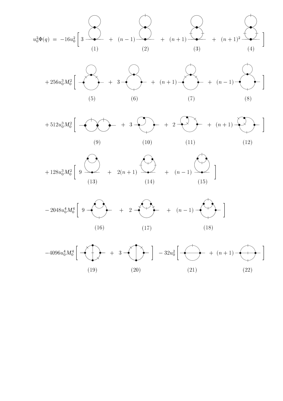
Figure 4: Two-loop diagrams for the two-point vertex function $\Gamma_{0T}^{(2)}(q)$, Eq. (86), with longitudinal and transverse propagators $G_{L}=$    and $G_{T}=$          , Eq. (27). The diagrams (5), (12), (17), (18), (19) and (22) contain Goldstone singularities for $h_{0}\to 0$ [see Eqs. (163)–(168)].

These diagrams are labelled by (1), (2), …, (22). The corresponding diagrams have also been given in Fig. 7 of Bervillier [57] where, however, our diagram (8) is missing and where the diagram corresponding to our diagram (4) has an incorrect prefactor. [These errors do not affect $\partial\Gamma_{0T}^{(2)}/\partial q^{2}|_{q=0}$, see Eq. (172).] Bervillier [57] calculated these diagrams within the $\epsilon=4-d$ expansion. Here we shall evaluate them in three dimensions.

We do not know of a rigorous proof of the equivalence between Josephson’s definition of $\rho_{s}$, Eq. (84), and the helicity modulus defined in Eqs. (65) and (66), but we shall verify this equivalence here in two-loop order by calculating $\partial\mathaccent 28695{\chi}_{{}_{T}}(q)^{-1}/\partial q^{2}|_{q=0}$ from Eq. (86). The result obtained for $\rho_{s}$ from Eq. (84) provides an important independent check of our calculation of the helicity modulus. Since the calculation is nontrivial we also provide some of the intermediate results in Appendix D. In particular, we present in Eqs. (163)–(168) the Goldstone divergencies. They are more complicated than those of $\Upsilon$ but they are finally cancelled in the sum of the diagrammatic contributions. When expressed as a function of $r_{0}^{\prime}$ we denote $\Gamma_{0T}^{(2)}(q)$ by $\mathaccent 28695{\Gamma}_{T}^{(2)}(q)$. After a long calculation, requiring considerably more computational effort than the calculation of $\Upsilon$ from the free energy, we obtain in three dimensions for $h_{0}\to 0$ and $r_{0}^{\prime}<0$

$$\left.\frac{\partial}{\partial q^{2}}\mathaccent 28695{\Gamma}_{T}^{(2)}(q)\right|_{q=0} = 1+\frac{2}{3\pi}u_{0}(-2r_{0}^{\prime})^{-1/2}+\frac{1}{3\pi^{2}}(\,18-n-24\ln 3\,)u_{0}^{2}(-2r_{0}^{\prime})^{-1}$$ (87)

$$\mbox{}+O(u_{0}^{3},u_{0}^{3}\ln u_{0})\,.$$

Eq. (87) contains no logarithms in $u_{0}$ since, at this order, there are no $d=3$ poles of $\partial\Gamma_{0T}^{(2)}(q)/\partial q^{2}|_{q=0}$. In terms of the correlation length $\xi_{-}$ we obtain

$$\left.\frac{\partial}{\partial q^{2}}\mathaccent 28695{\Gamma}_{T}^{(2)}(\xi_{-},u_{0},q,3)\right|_{q=0} = 1+\frac{2}{3\pi}u_{0}\xi_{-}+\frac{2}{3\pi^{2}}(\,8-n-12\ln 3\,)u_{0}^{2}\xi_{-}^{2}$$ (88)

$$+\,O(u_{0}^{3}\xi_{-}^{3})\,.$$

Using Eqs. (84) and (44) this indeed reproduces $\Upsilon(\xi_{-},u_{0},3)$ as given in Eq. (78) and thereby proves Eq. (66) up to two-loop order.

The renormalized vertex function $\Gamma_{T}^{(2)}$ is obtained from $\mathaccent 28695{\Gamma}_{T}^{(2)}$ according to

$$\Gamma_{T}^{(2)}(\xi_{-},u,\mu,q,d)=Z_{\phi}\mathaccent 28695{\Gamma}_{T}^{(2)}(\xi_{-},\mu^{\epsilon}A_{d}^{-1}Z_{u}Z_{\phi}^{-2}u,q,d)\,.$$ (89)

On the basis of dimensional arguments we define the dimensionless amplitude function $f_{T}$ as [17]

$$\left.\frac{\partial}{\partial q^{2}}\Gamma_{T}^{(2)}(\xi_{-},u,\mu,q,d)\right|_{q=0}=f_{T}(\mu\xi_{-},u,d)\,.$$ (90)

Using Eqs. (89) and (90) and substituting $Z_{u}(u,1)$ and $Z_{\phi}(u,1)$ we obtain in two-loop order in three dimensions

$$f_{T}(1,u,3)=1+\frac{8}{3}u+\left[\frac{488}{3}-4n-128\ln 3\right]u^{2}+O(u^{3})\,.$$ (91)

The first two terms agree with the earlier one-loop result [17, 39]. Multiplying Eq. (91) by the amplitude function $f_{\phi}$ in Eq. (52) we indeed recover Eq. (81) from Eqs. (66), (83) and (84) according to

$$G(1,u,3)=4\pi f_{\phi}(1,u,3)f_{T}(1,u,3)\,.$$ (92)

7 Results and discussion

Within the minimally renormalized field theory in three dimensions we have derived the two-loop contributions to the amplitude functions of the following $O(n)$ symmetric quantities of the $O(n)$ symmetric $\phi^{4}$ model at vanishing external field:

• the square of the order parameter $M_{0}^{2}=\langle\vec{\phi}_{0}\rangle^{2}$, Eq. (52),

• the helicity modulus $\Upsilon$, Eq. (81),

• the $q^{2}$ part of the inverse of the transverse susceptibility $\mathaccent 28695{\chi}_{{}_{T}}(q)$, Eq. (91), which yields the superfluid density $\rho_{s}$ (stiffness constant), Eq. (84),

• the specific heat $\mathaccent 28695{C}^{\pm}$ above and below $T_{\mathrm{c}}$, Eqs. (63) and (64).

Goldstone singularities arising in an intermediate stage of the calculations have been shown to cancel among themselves. The resulting amplitude functions are applicable to the asymptotic critical region as well as to the non-asymptotic region well away from criticality (apart from corrections arising from finite-cutoff effects, from $\phi^{6}$ terms and other higher-order couplings in $\cal H$, Eq. (1), and from analytic terms). They provide the basis for

• calculations of two-loop contributions to universal ratios $A_{i}/A_{k}$ and $a_{i}/a_{k}$ of leading and subleading amplitudes $A_{i}$ and $a_{i}$ which appear in the asymptotic representations [38]

  $$M_{0} = A_{{}_{M}}|t|^{\beta}\left(1+a_{{}_{M}}|t|^{\Delta}+\ldots\right)\,,$$ (93)

  $$\rho_{s} = A_{\rho_{s}}|t|^{(d-2)\nu}\left(1+a_{\rho_{s}}|t|^{\Delta}+\ldots\right)\,,$$ (94)

  $$\mathaccent 28695{C}^{\pm} = B+\frac{A^{\pm}}{\alpha}|t|^{-\alpha}\left(1+a_{{}_{C}}^{\pm}|t|^{\Delta}+\ldots\right)\,,$$ (95)

• nonlinear RG analyses of non-asymptotic critical phenomena of O($n$) symmetric systems above and below $T_{\mathrm{c}}$ (for the general strategy of such analyses see Ref. [19]).

These applications are of particular relevance to future experimental tests of the RG predictions of critical-point universality along the $\lambda$ line of ⁴He $(n=2)$ [37].

The various amplitude functions are plotted in Figs. 5–9 vs the renormalized coupling $u$ for the examples $n=1$ and $n=2$. In order to indicate the relative magnitude of the two-loop contributions we have also plotted the corresponding zero- and one-loop approximations and, where available, the Borel resummed results (for $n=1$ and $n=2$ above $T_{\mathrm{c}}$ [22] and for $n=1$ below $T_{\mathrm{c}}$ [23]). The curves terminate at the fixed points [16] $u^{\star}=0.0405$ for $n=1$ and $u^{\star}=0.0362$ for $n=2$ (although extensions to $u>u^{\star}$ may be needed in certain cases [21, 44, 45]). We comment on these curves as follows.

Figure 5: Amplitude function $G(u)\equiv G(1,u,3)$ for the superfluid density ($n=2$), Eq. (81), multiplied by $u$, as a function of the renormalized coupling $u$ in zero-, one- and two-loop order.

For the superfluid density $(n=2)$, the one- and two-loop corrections for $G(1,u,3)$, see Fig. 5, each contribute about 10% of the zero-loop term $1/8u^{\star}$ at the fixed point. (For $n=3$ corresponding corrections are about 9% and 5%, respectively, at $u^{\star}=0.0328$.) The fact that the one- and two-loop contributions are of comparable magnitude suggests that higher-loop calculations including a Padé-type analysis or a Borel resummation are necessary before a reliable quantitative prediction can be made for amplitude ratios such as [17] $R_{\xi}^{T}$ or $a_{{}_{C}}^{-}/a_{\rho_{s}}$. A preliminary analysis [61] of experimental data [62, 63] for $\rho_{s}$ and $\mathaccent 28695{C}^{\pm}$, similar to the analyses in Refs. [19, 39, 64], indicate that the one-loop approximation for $G(1,u^{\star},3)$ is closer to the experimental result than the two-loop approximation. Since $G(1,u,3)$ can be considered as consisting of two factors $4\pi f_{\phi}$ and $f_{T}$ according to Eq. (92), it is interesting to discuss the latter amplitude functions separately.

Figure 6: Amplitude function $f_{\phi}(u)\equiv f_{\phi}(1,u,3)$ for the square of the order parameter ($n=1,\>2$), Eq. (52), multiplied by $u$, as a function of the renormalized coupling $u$ in zero-, one- and two-loop order. The dot-dashed curve is the Borel summation result given for $n=1$ in Ref. [23].

For the order parameter, we first consider $f_{\phi}$ for the case $n=1$ for which the Borel summation result is known [23]. It is shown in Fig. 6 as the dot-dashed curve. As pointed out previously [23], the Borel result deviates only very little (by about 3% at the fixed point) from the zero- and one-loop result whereas the two-loop result is about 15% larger at $u^{\star}$. Obviously, the leading order approximation is the better one in this case. We conjecture that this feature of the leading term will remain true also when $n>1$ since the zero-loop term does not depend on $n$ and since the one-loop term vanishes for general $n$ [due to the choice of the geometric factor $A_{d}$ in Eq. (9)]. We note that for $n=2$ the two-loop result for $f_{\phi}$ shown in Fig. 6 lies about 9% above the zero- and one-loop results, similar to the two-loop term for the case $n=1$. Our experience with other amplitude functions above $T_{\mathrm{c}}$ for which Borel summation results are available [22] is that the order in perturbation theory which is closest to the Borel results seems to be the same for $n=1$, 2, 3. Clearly, in order to make reliable quantitative predictions a higher-order calculation and Borel summation of the order parameter for $n>1$ are necessary.

Figure 7: Amplitude function $f_{T}(u)\equiv f_{T}(1,u,3)$ for $\partial\mathaccent 28695{\chi}_{{}_{T}}(q)^{-1}/\partial q^{2}|_{q=0}$ for $n=2$, Eq. (91), as a function of the renormalized coupling $u$ in zero-, one- and two-loop order.

Consider now the amplitude function $f_{T}$ of the transverse susceptibility shown in Fig. 7. For $n=2$, the one-loop contribution at $u^{\star}$ is about 10% whereas the two-loop correction is much smaller, being only about 1%. (For $n=3$ the corresponding corrections are about 9% and 1%, respectively.) We regard the smallness of the two-loop term as an indication of the quantitative reliability of the low-order formula for $f_{T}$ in Eq. (91). We infer from this and from our observations for $f_{\phi}$ that the considerable two-loop contribution to the amplitude function $G$ is mostly due to the large two-loop term in $f_{\phi}$ and hence that the one-loop approximation for $G$ is probably the most reliable at the present time. A substantiation of this conjecture by higher-order calculations and Borel resummations would be highly desirable. From a practical point of view, the presumed reliability of the low-order result of $f_{T}$ is quite important since higher-order calculations of $f_{\phi}$ for $n>1$ require considerably less computational effort than those of $f_{T}$ or of $G$. Thus, in a first step of future calculations of the amplitude function of the superfluid density, it will be sufficient to perform higher-order calculations only of $f_{\phi}$ for $n>1$ before embarking on a long-term project of much more difficult higher-order calculations of $\mathaccent 28695{\chi}_{{}_{T}}(q)$ or of $\Upsilon$. We consider this important conclusion as a major result of our two-loop analysis.

These considerations give some support to the good agreement obtained previously [39] between the one-loop formula for the superfluid density and experimental data [62, 63] for ⁴He in the (nonasymptotic) temperature range $10^{-6}\,\raisebox{-2.84526pt}{$\stackrel{{\scriptstyle{\textstyle<}}}{{{\textstyle\sim}}}$}\,t\,\raisebox{-2.84526pt}{$\stackrel{{\scriptstyle{\textstyle<}}}{{{\textstyle\sim}}}$}\,10^{-2}$ at several pressures near the $\lambda$-line. A quantitative description of the nonasymptotic region, however, depends not only on amplitude functions like $G$ but also, crucially, on an accurate knowledge of the effective coupling $u(l)$, which can be obtained from the experimentally determined specific heat [14, 64] . The formulas used to extract the nonuniversal initial value of the effective coupling as a function of the pressure involve not only the RG exponent functions, which are known accurately from Borel summations [16], but also the amplitude functions of the specific heat $F_{\pm}(1,u,3)$, which are given here to two-loop order in Eqs. (63) and (64).

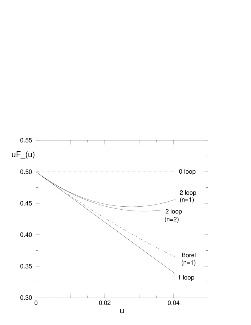
Figure 8: Amplitude function $F_{-}(u)\equiv F_{-}(1,u,3)$ for the specific heat below $T_{\mathrm{c}}$ ($n=$1, 2), Eq. (64), multiplied by $u$, as a function of the renormalized coupling $u$ in zero-, one- and two-loop order. The dot-dashed curve is the Borel summation result given for $n=1$ in Ref. [23].

Figure 9: Amplitude function $F_{+}(u)\equiv F_{+}(1,u,3)$ for the specific heat above $T_{\mathrm{c}}$ ($n=$1, 2), Eq. (63), as a function of the renormalized coupling $u$ in one- and two-loop order. The dot-dashed curves are the Borel summation results given in Ref. [22].

Figure 8 shows the amplitude function $F_{-}$ of the specific heat below $T_{\mathrm{c}}$ as a function of the renormalized coupling. As for the order parameter, we may use the known Borel summation results [23] for $n=1$ (dot-dashed curve in Fig. 7) to infer the reliability of the low order approximations for $n=2$. As noted previously [23], the one-loop approximation is the better one, differing from the Borel result at the fixed point by about 5% of the zero-loop term $1/2u^{\star}$ compared with about 16% for the two-loop result. Evidently, the derivative of $F_{-}$ at $u=u^{\star}$, which is needed for universal correction-to-scaling ratios [17], is also not well-approximated at two-loop order. Thus higher-order calculations of $F_{-}$ for $n>1$ are urgently needed.

In Fig. 9, we plot the amplitude function $F_{+}$ of the specific heat above $T_{\mathrm{c}}$, where Borel results are available for $n\geq 1$, as a function of the renormalized coupling [22]. Here, it is the two-loop rather than the one-loop approximation which is closer to the Borel results. This demonstrates that it is not clear a priori which (low) order of perturbation theory will provide the best approximation.

Let us note finally that the Borel results [22, 23] for $F_{+}$ ($n\geq 1$) and for $F_{-}$ ($n=1$) in three dimensions neglect the leading poles (in four dimensions) of the additive renormalization $A(u,\epsilon)$ in Eq. (60) beyond two-loop order. Since a resummation of the (as yet unknown) higher-order terms in the RG function $B(u)$ associated with $A(u,\epsilon)$ (see Eqs. (2.32) and (2.33) in Ref. [17]) is expected to yield a small correction [65] of O($\eta$), we do not expect these Borel results for $F_{\pm}$ to be affected strongly by this approximation [22]. However, at the level of accuracy anticipated in future experiments [37], it is likely that the present uncertainties regarding $B(u)$ will become significant, thus $B(u)$ itself will also be needed with the improved accuracy provided by a resummation of its high-order perturbation series. We recall that the function $B(u)$ enters not only the formulas for the universal amplitude ratios [17, 38] such as $A^{+}/A^{-},\>R^{T}_{\xi},\>a_{{}_{C}}^{+}/a_{{}_{C}}^{-}$ and $a_{{}_{C}}^{-}/a_{\rho_{s}}$ but also the formulas needed to determine the effective coupling $u(l)$ from the specific heat [14, 19, 64].

In conclusion, our new two-loop results for $n>1$ below $T_{\mathrm{c}}$ provide additional motivation and specific information on the strategy and direction of higher-order calculations planned for future theoretical research parallel to the considerable effort on the experimental side to test the fundamental law of critical-point universality [37].

Appendix A Correlation lengths

In this Appendix we derive Eqs. (13) and (14) and relate $\xi_{\pm}$ to $t$. Above $T_{\mathrm{c}}$, we obtain $\xi_{+}$ from Eq. (12) and the two-point vertex function [16] $\Gamma_{0}^{(2)}(q,r_{0},u_{0})=\mathaccent 28695{\chi}_{+}(q)^{-1}$. In two-loop order we have

$$\Gamma_{0}^{(2)}(q,r_{0},u_{0})=r_{0}+q^{2}-\frac{4}{\epsilon}(n+2)A_{d}u_{0}r_{0}^{1-\epsilon/2}+\frac{16}{\epsilon^{2}}(n+2)^{2}(1-\frac{\epsilon}{2})A_{d}^{2}u_{0}^{2}r_{0}^{1-\epsilon}$$ (96)

$$- 32(n+2)\frac{\Gamma(\epsilon)}{(4\pi)^{d}}\left[\frac{J_{0}(\epsilon)}{\epsilon-1}-J_{2}(\epsilon)q^{2}+O(q^{4})\right]u_{0}^{2}r_{0}^{1-\epsilon}+O(u_{0}^{3})\,,$$

$$J_{0}(\epsilon) = \int_{0}^{1}\mbox{d}x\int_{0}^{1}\mbox{d}y\frac{y^{\epsilon/2-1}}{[1-y+y(x-x^{2})]^{2-\epsilon/2}}\,,$$ (97)

$$J_{2}(\epsilon) = \int_{0}^{1}\mbox{d}x\int_{0}^{1}\mbox{d}y\frac{y^{\epsilon/2}(1-y)(x-x^{2})}{[1-y+y(x-x^{2})]^{3-\epsilon/2}}$$ (98)

which leads to

$$\xi_{+}^{-2} = r_{0}\left\{1-4(n+2)\frac{1}{\epsilon}A_{d}u_{0}r_{0}^{-\epsilon/2}+16(n+2)^{2}\left[\frac{1}{\epsilon^{2}}-\frac{1}{2\epsilon}\right]A_{d}^{2}u_{0}^{2}r_{0}^{-\epsilon}\right.$$ (99)

$$\phantom{r_{0}\Big{[}}-\left.a_{2}(\epsilon)u_{0}^{2}r_{0}^{-\epsilon}+O(u_{0}^{3})\right\}\,,$$

$$a_{2}(\epsilon) = 32(n+2)\Gamma(\epsilon)(4\pi)^{-d}\left[J_{0}(\epsilon)(\epsilon-1)^{-1}+J_{2}(\epsilon)\right]$$ (100)

where $J_{0}(1)=2\pi$ and $J_{2}(1)=2\pi/27$. Inversion of Eq. (99) gives for $\xi_{+}^{-2}\not=0$

$$r_{0} = \xi_{+}^{-2}\left[1+4(n+2)\frac{1}{\epsilon}A_{d}u_{0}\xi_{+}^{\epsilon}+a_{2}(\epsilon)(u_{0}\xi_{+}^{\epsilon})^{2}+O\!\left((u_{0}\xi_{+}^{\epsilon})^{3}\right)\right]\,,$$ (101)

where

$$a_{2}(\epsilon)=\frac{n+2}{\pi^{2}}(\epsilon-1)^{-1}\left[1+O(\epsilon-1)\right]$$ (102)

determines the coefficient of the $d=3$ pole of $r_{0{\mathrm{c}}}$ in Eq. (10). Subtracting $\delta r_{0}=r_{0}-r_{0}^{\prime}$ [see Eq. (11)] from Eq. (101) and letting $\epsilon\rightarrow 1$ we obtain

$$r_{0}^{\prime} = \xi_{+}^{-2}\,\Bigg{\{}\,1+\frac{1}{\pi}(n+2)u_{0}\xi_{+}+\frac{1}{27\pi^{2}}(n+2)(u_{0}\xi_{+})^{2}\left[1+54\ln(24u_{0}\xi_{+})\right]$$ (103)

$$+\left[32(n+2)\frac{\partial}{\partial\epsilon}\left.\frac{\Gamma(\epsilon)}{(4\pi)^{d}}J_{0}(\epsilon)\right|_{\epsilon=1}\!\!\!-\frac{2}{\pi^{2}}(n+2)\ln 24-C(n)\,\right](u_{0}\xi_{+})^{2}$$

$$+\,O(u_{0}^{3},u_{0}^{3}\ln u_{0})\,\Bigg{\}}\,.$$

Here we have added and subtracted a logarithmic term $2\pi^{-2}(n+2)(u_{0}\xi_{+})^{2}\ln 24$ in order to conform with the representation of $r_{0}^{\prime}$ in Refs. [11] and [23] for $n=1$ in terms of the bare coupling $g_{0}=24u_{0}$ of Ref. [11]. Now a convenient choice for $C(n)$ is such that the term in the square brackets of Eq. (103) vanishes, i. e.

$$C(n)=\frac{1}{\pi^{2}}(n+2)\left[1-C_{\mathrm{E}uler}+\ln\frac{4\pi}{9}-2\ln 24\right]\,.$$ (104)

This yields Eq. (13) and corresponds to the choice $C_{1}=0$ in Eq. (A2) of Ref. [11] for $n=1$.

Below $T_{\mathrm{c}}$, $\xi_{-}$ is defined, according to Eqs. (3.1)–(3.6) of Ref. [17], as

$$r_{0}^{\prime}=\xi_{-}^{-2}R_{0+}(u_{0}\xi_{-}^{\epsilon},\epsilon)-\frac{3}{2}\xi_{-}^{-2}Z_{r}(u(l_{-}),\epsilon)-\delta r_{0}\,,$$ (105)

(see also Eq. (A4) in Ref. [23]) where the function $R_{0+}(u_{0}\xi_{+}^{\epsilon},\epsilon)$ is defined above $T_{\mathrm{c}}$ and represents the series of $r_{0}$ in integer powers of $u_{0}\xi_{+}^{\epsilon}$ whose first three terms are given in the square brackets of Eq. (101). The effective coupling $u(l_{-})$ as a function of the flow parameter $l_{-}$ is determined by Eq. (110) below. For $\epsilon=1$, the function $\xi_{-}^{-2}R_{0+}(u_{0}\xi_{-},1)-\delta r_{0}$ can be read off, up to two-loop order, from the right-hand side of Eq. (13) which represents $\xi_{+}^{-2}R_{0+}(u_{0}\xi_{+},1)-\delta r_{0}$. Thus it remains to rewrite $Z_{r}(u(l_{-}),1)$ as a function of $u_{0}\xi_{-}$ (see Eq. (A7) of Ref. [23]). This leads to Eq. (14).

The connection between $\xi_{\pm}$ and $t$ is given by [16, 17]

$$at = \xi_{+}^{-2}\,Q_{+}(1,u(l_{+}),d)\,\exp\int_{l_{+}}^{1}\zeta_{r}(u(l))\frac{dl}{l},\quad t>0,$$ (106)

$$-2at = \xi_{-}^{-2}\,Q_{-}(1,u(l_{-}),d)\,\exp\int_{l_{-}}^{1}\zeta_{r}(u(l))\frac{dl}{l},\quad t<0,$$ (107)

$$a = Z_{r}(u,\epsilon)^{-1}a_{0}\,,$$ (108)

$$\zeta_{r}(u) = \left.\mu\partial_{\mu}\ln Z_{r}(u,\epsilon)^{-1}\right|_{0}\,,$$ (109)

$$l_{\pm}{\d}u(l_{\pm})/{\d}l_{\pm} = \beta_{u}(u(l_{\pm}),\epsilon)\,,$$ (110)

where $Q_{\pm}(1,u,d)$ are the amplitude functions of the correlation lengths $\xi_{\pm}$. They are related according to $Q_{-}(1,u,d)=3-2Q_{+}(1,u,d)$. A convenient representation for $Q_{+}(1,u,3)$ is given in Eq. (3.5) of Ref. [22].

Appendix B Diagrams of $\Gamma_{0}^{(1)}$

In this appendix, we show the cancellation of (spurious) Goldstone divergences when the order parameter is calculated from the one-point vertex function $\Gamma_{0}^{(1)}(r_{0},u_{0},M_{0})=h_{0}$ as given by the sum of 1PI diagrams with one amputated external leg. These diagrams have been given to two-loop order by Bervillier in Fig. 5 of Ref. [57] and by Shpot in Eq. (17) of Ref. [51] where they were evaluated by use of an $\epsilon=4-d$ expansion. Here we shall work at $d=3$. The analytic expression,up to order $O(u_{0}^{2})$, is

$$\frac{h_{0}}{M_{0}}=r_{0}+4u_{0}M_{0}^{2}+12u_{0}\int_{\bf p}G_{L}(p)+4(n-1)u_{0}\int_{\bf p}G_{T}(p)+u_{0}^{2}Y_{0}$$ (111)

where $Y_{0}=Y_{0a}+Y_{0b}+\ldots+Y_{0i}$ is the sum of the two-loop contributions

$$Y_{0a} = -144\int_{\bf p_{1}}G_{L}(p_{1})\int_{\bf p_{2}}G_{L}(p_{2})^{2}\,,$$ (112)

$$Y_{0b} = -48(n-1)\int_{\bf p_{1}}G_{T}(p_{1})\int_{\bf p_{2}}G_{L}(p_{2})^{2}\,,$$ (113)

$$Y_{0c} = -16(n-1)\int_{\bf p_{1}}G_{L}(p_{1})\int_{\bf p_{2}}G_{T}(p_{2})^{2}\,,$$ (114)

$$Y_{0d} = -16(n^{2}-1)\int_{\bf p_{1}}G_{T}(p_{1})\int_{\bf p_{2}}G_{T}(p_{2})^{2}\,,$$ (115)

$$Y_{0e} = -96\int_{\bf p_{1}}\int_{\bf p_{2}}G_{L}(p_{1})\,G_{L}(p_{2})\,G_{L}(|\bf p_{1}\!+\!p_{2}|)\,,$$ (116)

$$Y_{0f} = -32(n-1)\int_{\bf p_{1}}\int_{\bf p_{2}}G_{T}(p_{1})\,G_{T}(p_{2})\,G_{L}(|\bf p_{1}\!+\!p_{2}|)\,,$$ (117)

$$Y_{0g} = 3456u_{0}M_{0}^{2}\int_{\bf p_{1}}\int_{\bf p_{2}}G_{L}(p_{1})^{2}\,G_{L}(p_{2})\,G_{L}(|\bf p_{1}\!+\!p_{2}|)\,,$$ (118)

$$Y_{0h} = 384(n-1)u_{0}M_{0}^{2}\int_{\bf p_{1}}\int_{\bf p_{2}}G_{T}(p_{1})\,G_{T}(p_{2})\,G_{L}(|{\bf p_{1}\!+\!p_{2}}|)^{2}\,,$$ (119)

$$Y_{0i} = 256(n-1)u_{0}M_{0}^{2}\int_{\bf p_{1}}\int_{\bf p_{2}}G_{T}(p_{1})^{2}\,G_{T}(p_{2})\,G_{L}(|\bf p_{1}\!+\!p_{2}|)$$ (120)

with $G_{L}(p)$ and $G_{T}(p)$ given by Eq. (27). Eqs. (111)–(119) agree with Refs. [51] and [57]. The prefactor $256(n-1)u_{0}M_{0}^{2}$ in Eq. (120) agrees with the prefactor of the corresponding diagram of Shpot [51] who corrected the corresponding prefactor of Bervillier [57].

The quantities $Y_{0e}$ and $Y_{0f}$ contain $d=3$ poles, but since $Y_{0e}=2(u_{0}^{2}M_{0}^{2})^{-1}X_{0H}$ and $Y_{0f}=2(u_{0}^{2}M_{0}^{2})^{-1}(X_{0I}+X_{0J})$ for $k=0$ [see Eqs. (132)–(134)], the substitution $r_{0}=r_{0}^{\prime}+\delta r_{0}$ in Eq. (111) leads to the cancellation of these poles in the same way as in Eq. (29). Thus,

$$\lim_{\epsilon\to 1}\,\left[\delta r_{0}+u_{0}^{2}(\mathaccent 28695{Y}_{e}+\mathaccent 28695{Y}_{f})\right]=2u_{0}^{2}f(r_{0}^{\prime},u_{0},M_{0})$$ (121)

with $f(r_{0}^{\prime},u_{0},M_{0})$ given by Eq. (33). At this stage, one has the choice of performing the integrations before or after solving iteratively for $M_{0}^{2}$. Carrying out the integrations first, one is led to Eq. (36). Inverting first, one finds

$$M_{0}^{2} = \frac{1}{4u_{0}}(-r_{0}^{\prime}+\mathaccent 28695{\chi}_{{}_{T}}^{-1})+\frac{3}{4\pi}(-2r_{0}^{\prime}+3\mathaccent 28695{\chi}_{{}_{T}}^{-1})^{1/2}+\frac{1}{4\pi}(n-1)\mathaccent 28695{\chi}_{{}_{T}}^{-1/2}+u_{0}\mathaccent 28695{Y}_{1}$$ (122)

$$-\,\frac{u_{0}}{4}\left[\mathaccent 28695{Y}-\mathaccent 28695{Y}_{e}-\mathaccent 28695{Y}_{f}\right]-\frac{u_{0}}{2}\tilde{f}(r_{0}^{\prime},u_{0},\mathaccent 28695{\chi}_{{}_{T}})+O(u_{0}^{2},u_{0}^{2}\ln u_{0})$$

where

$$\tilde{f}(r_{0}^{\prime},u_{0},\mathaccent 28695{\chi}_{{}_{T}})=\frac{n+2}{\pi^{2}}\ln\frac{(-2r_{0}^{\prime}+3\mathaccent 28695{\chi}_{{}_{T}}^{-1})^{1/2}}{24u_{0}}+\frac{n-1}{\pi^{2}}\ln\frac{1+2w^{1/2}}{3}\,,$$ (123)

with $w$ given by Eq. (38), that is, $\tilde{f}=f$ in Eq. (33) in lowest order in $u_{0}$, and

$$u_{0}\mathaccent 28695{Y}_{1} = \frac{u_{0}}{8\pi^{2}}\left\{27+(n-1)\left[n-1+9w^{1/2}+3w^{-1/2}\right]\right\}$$ (124)

is the $O(u_{0})$ contribution from the expansion of the integrals in Eq. (111) at one-loop order. In three dimensions we obtain for finite $w$

$$\mathaccent 28695{Y}_{a} = 9\,(2\pi^{2})^{-1}\,,$$ (125)

$$\mathaccent 28695{Y}_{b} = 3\,(2\pi^{2})^{-1}(n-1)w^{1/2}\,,$$ (126)

$$\mathaccent 28695{Y}_{c} = (2\pi^{2})^{-1}(n-1)w^{-1/2}\,,$$ (127)

$$\mathaccent 28695{Y}_{d} = (2\pi^{2})^{-1}(n^{2}-1)\,,$$ (128)

$$\mathaccent 28695{Y}_{g} = 9\,(2\pi^{2})^{-1}(1-w)\,,$$ (129)

$$\mathaccent 28695{Y}_{h} = 3\,(2\pi^{2})^{-1}(n-1)(1-2w^{1/2})(1-w)(1-4w)^{-1}\,,$$ (130)

$$\mathaccent 28695{Y}_{i} = \pi^{-2}(n-1)(w^{-1/2}-2)(1-w)(1-4w)^{-1}\,.$$ (131)

Goldstone divergences $\sim w^{-1/2}$ arise from Eqs. (124), (127), and (131) for $h_{0}\to 0$. They cancel among themselves in $\mathaccent 28695{Y}_{1}-{\textstyle\frac{1}{4}}(\mathaccent 28695{Y}_{c}+\mathaccent 28695{Y}_{i})$. Summing the remaining terms, one obtains the same result, Eq. (37), as derived via the free energy $\mathaccent 28695{\Gamma}$.

Appendix C Two-loop diagrams of $\Gamma_{0}$ at $\bf k\not=0$

The contributions $X_{0A}$, $X_{0B}$, …, $X_{0L}$ in Eq. (28) at finite $k$ are represented by the two-loop diagrams in Fig. 3. Diagrams A–G consist of products of exactly calculable one-loop integrals [24]. The integral expressions of the diagrams H–L read

$$X_{0H} = -48u_{0}^{2}M_{0}^{2}\int_{\bf p_{1}}\int_{\bf p_{2}}R_{L}(p_{1})\,R_{L}(p_{2})\,R_{L}(|{\bf p_{1}+p_{2}}|)\,,$$ (132)

$$X_{0I} = -16u_{0}^{2}M_{0}^{2}\int_{\bf p_{1}}\int_{\bf p_{2}}R_{T}(p_{1})\,R_{T}(p_{2})\,R_{L}(|{\bf p_{1}+p_{2}}|)\,,$$ (133)

$$X_{0J} = -16(n-2)u_{0}^{2}M_{0}^{2}\int_{\bf p_{1}}\int_{\bf p_{2}}G_{T}(p_{1})\,G_{T}(p_{2})\,R_{L}(|{\bf p_{1}+p_{2}}|)\,,$$ (134)

$$X_{0K} = -96u_{0}^{2}M_{0}^{2}\int_{\bf p_{1}}\int_{\bf p_{2}}R_{LT}(p_{1})\,R_{LT}(p_{2})\,R_{L}(|{\bf p_{1}+p_{2}}|)\,,$$ (135)

$$X_{0L} = -32u_{0}^{2}M_{0}^{2}\int_{\bf p_{1}}\int_{\bf p_{2}}R_{LT}(p_{1})\,R_{TL}(p_{2})\,R_{T}(|{\bf p_{1}+p_{2}}|)\,.$$ (136)

Here we have used the elements of the matrix $K^{-1}$ of $\mathbf{k}$-dependent propagators

$$K({\mathbf{p},k})^{-1} = \left(\begin{array}[]{cc}R_{L}(p)&R_{LT}(p)\\ R_{TL}(p)&R_{T}(p)\end{array}\right)\,,$$ (139)

$$R_{L}(p) = \frac{\bar{r}_{0T}+p^{2}+k^{2}}{\det K({\bf p,k})}\,,\qquad R_{LT}(p)=\frac{-2i\,\bf k\!\cdot\!p}{\det K({\bf p,k})}\,,$$ (140)

$$R_{T}(p) = \frac{\bar{r}_{0L}+p^{2}+k^{2}}{\det K({\bf p,k})}\,,\qquad R_{TL}(p)=-R_{LT}(p)$$ (141)

where $K(\bf p,k)$, $\bar{r}_{0L}$, $\bar{r}_{0T}$, $G_{L}(p)$ and $G_{T}(p)$ are given in Eqs. (25)–(27), respectively. The contributions $\partial\mathaccent 28695{X}_{j}/\partial k^{2}|_{k=0}$ to the helicity modulus, Eq. (69), will be denoted by $\partial_{k^{2}}\mathaccent 28695{X}_{j}$. The quantities $\partial_{k^{2}}\mathaccent 28695{X}_{C}=\partial_{k^{2}}[2u_{0}\int_{\bf p_{1}}R_{L}(p_{1})\int_{\bf p_{2}}R_{T}(p_{2})]$ and $\partial_{k^{2}}\mathaccent 28695{X}_{I}$ are divergent for $h_{0}\to 0$. While $\partial_{k^{2}}\mathaccent 28695{X}_{C}$ is easily evaluated in terms of standard one-loop integrals, $\partial_{k^{2}}\mathaccent 28695{X}_{I}$ is given, in three dimensions, by

$$2\partial_{k^{2}}\mathaccent 28695{X}_{I} = \frac{-4/3}{(4\pi)^{3}}\,u_{0}\Big{[}\,8(1+\alpha)I_{1}+(1+4\alpha)I_{2}+4\alpha I_{3}-(6+8\alpha)I_{4}\,\Big{]}\,,$$ (142)

$$I_{i} = \int_{0}^{1}{\d}x\int_{0}^{1}{\d}y\>\frac{y^{-1/2}\,f_{i}(x,y)}{[1-y+y(x-x^{2})]^{3/2}}\,,$$ (143)

$$f_{1}(x,y) = \ln(y+\alpha)-\ln(1-y+\alpha)\,,\quad f_{2}(x,y)=xy\,(xy+\alpha)^{-1}\,,$$ (144)

$$f_{3}(x,y) = \ln\alpha-\ln(1-y+\alpha)\,,\quad f_{4}(x,y)=xy\,(1-y+\alpha)^{-1}\,,$$ (145)

where $\alpha$ is given by Eq. (73). To illustrate the evaluation of these integrals, we consider $I_{4}$. Thus,

$$I_{4} = \int_{0}^{1}{\d}x\int_{0}^{1}{\d}y\frac{y^{1/2}x\,(1-y+\alpha)^{-1}}{[1-y+y(x-x^{2})]^{3/2}}$$ (146)

$$= \int_{1/4}^{\infty}{\d}z\int_{0}^{1/2}{\d}u\frac{(z-u^{2})^{3/2}}{[z-1/4+\alpha(z+3/4)]}$$ (147)

$$= \int_{1/4}^{\infty}\frac{{\d}z}{z}\,\frac{(4z-1)^{-1/2}}{[z-1/4+\alpha(z+3/4)]}$$ (148)

$$= \frac{8}{1+\alpha}\int_{0}^{\infty}{\d}t\,\,\frac{1}{(t^{2}+1)}\,\frac{1}{(t^{2}+4\alpha(1+\alpha)^{-1})}$$ (149)

$$= \frac{2\pi}{1-3\alpha}\left[\alpha^{-1/2}(1+\alpha)^{1/2}-2\right]\,.$$ (150)

In going from (146) to (150) we have used the substitutions $z=y^{-1}-3/4$, $u=x-1/2$, then $u=z^{1/2}\sin w$ and finally $z=(t^{2}+1)/4$. While $I_{4}$ exhibits a divergence for $h_{0}\to 0$, the other contributions to $\partial_{k^{2}}\mathaccent 28695{X}_{I}$ are finite in this limit and lead to Eq. (75).

The remaining contributions are finite for $h_{0}\to 0$. For $j=$ A, B and F they are readily evaluated in three dimensions as

$$2\partial_{k^{2}}\mathaccent 28695{X}_{A} = \textstyle 2\partial_{k^{2}}\Big{[}3u_{0}\left(\int_{\bf p}R_{L}(p)\right)^{2}\Big{]}=-(8\pi^{2})^{-1}u_{0}\,,$$ (151)

$$2\partial_{k^{2}}\mathaccent 28695{X}_{B} = \textstyle 2\partial_{k^{2}}\Big{[}3u_{0}\left(\int_{\bf p}R_{T}(p)\right)^{2}\Big{]}=3\,(8\pi^{2})^{-1}u_{0}\,,$$ (152)

$$2\partial_{k^{2}}\mathaccent 28695{X}_{F} = \textstyle 2\partial_{k^{2}}\Big{[}2(n-2)u_{0}\int_{\bf p_{1}}\!R_{T}(p_{1})\!\int_{\bf p_{2}}\!G_{T}(p_{2})\Big{]}=(8\pi^{2})^{-1}(n-2)u_{0}\,.$$ (153)

$\partial_{k^{2}}\mathaccent 28695{X}_{E}=\partial_{k^{2}}[2(n-2)u_{0}\int_{\bf p_{1}}R_{L}(p_{1})\int_{\bf p_{2}}G_{T}(p_{2})]$ vanishes for $h_{0}\to 0$, $\mathaccent 28695{X}_{G}=n(n-2)u_{0}\,[\int_{\bf p}G_{T}(p)]^{2}$ is $k$-independent, and $\mathaccent 28695{X}_{D}=4u_{0}\,[\int_{\bf p}R_{LT}(p)]^{2}=0$. For $j=$ H, J, K and L we use splitting by partial fraction and obtain in three dimensions for $h_{0}\to 0$

$$2\partial_{k^{2}}\mathaccent 28695{X}_{H} = -(8\pi^{2})^{-1}u_{0}\,,$$ (154)

$$2\partial_{k^{2}}\mathaccent 28695{X}_{J} = -(24\pi^{2})^{-1}(n-2)u_{0}\,,$$ (155)

$$2\partial_{k^{2}}\mathaccent 28695{X}_{K} = \pi^{-2}(1-\ln 3)u_{0}\,,$$ (156)

$$2\partial_{k^{2}}\mathaccent 28695{X}_{L} = (3\pi^{2})^{-1}(2\ln 2-1)u_{0}\,.$$ (157)

Appendix D Contributions to $\partial\Gamma_{0T}^{(2)}/\partial q^{2}$

We denote the integral expressions of the two-loop contribution $\Phi(q)$ in Eq. (86) by $\Phi_{i}$, $i=1$, 2, …, 22. The derivative of $\Gamma_{0T}^{(2)}$ with respect to $q^{2}$ at $q=0$ yields

$$\left.\partial_{q^{2}}\Gamma_{0T}^{(2)}(q)\right|_{q=0} = 1+u_{0}\Psi+u_{0}^{2}\left.\partial_{q^{2}}\,\Phi(q)\right|_{q=0}+O(u_{0}^{3})\,,$$ (158)

$$\Psi = \frac{8}{d}\cdot\frac{\epsilon\bar{r}_{0T}+d\bar{r}_{0L}}{(\bar{r}_{0L}-\bar{r}_{0T})^{2}}\int_{\bf p}\left[G_{T}(p)-G_{L}(p)-(\bar{r}_{0L}-\bar{r}_{0T})G_{L}(p)^{2}\right]$$ (159)

$$-\,\frac{32}{d}\bar{r}_{0L}\int_{\bf p}\!G_{L}(p)^{3}\,.$$

Expanding $\Psi$ with respect to $u_{0}$ and replacing $r_{0}$ by $r_{0}^{\prime}$ we obtain in three dimensions

$$u_{0}\Psi = \frac{2}{3\pi}u_{0}\tau\left[1+O(\alpha^{1/2})\right]+u_{0}^{2}\Psi_{1}+O(u_{0}^{3})\,,$$ (160)

$$\Psi_{1} = -\frac{1}{\pi^{2}}\tau^{2}\left[3\alpha^{-1/2}+n-8+O(\alpha^{1/2})\right]\,,$$ (161)

$$\tau = (-2r_{0}^{\prime}+2\mathaccent 28695{\chi}_{{}_{T}}^{-1})^{-1/2}\,.$$ (162)

Eq. (161) exhibits a Goldstone singularity $\sim\alpha^{-1/2}$ with $\alpha$ given by Eq. (73). Further Goldstone singularities are contained in the two-loop diagrams (5), (12), (17), (18), (19) and (22) in Fig. 4. We find, in three dimensions,

$$\partial_{q^{2}}\Phi_{5} = \pi^{-2}\tau^{2}\left[\alpha^{-1/2}-4+O(\alpha^{1/2})\right],$$ (163)

$$\partial_{q^{2}}\Phi_{12} = -2\,(27\pi^{2})^{-1}(n+1)\tau^{2}\left[\alpha^{-1}-9\ln(9\alpha)-12+O(\alpha^{1/2})\right],$$ (164)

$$\partial_{q^{2}}\Phi_{17} = (6\pi^{2})^{-1}\tau^{2}\left[12\alpha^{-1/2}-7-80\ln 2+O(\alpha^{1/2})\right],$$ (165)

$$\partial_{q^{2}}\Phi_{18} = (27\pi^{2})^{-1}(n-1)\tau^{2}\left[\alpha^{-1}-18\ln(9\alpha)-33+O(\alpha^{1/2})\right],$$ (166)

$$\partial_{q^{2}}\Phi_{19} = (54\pi^{2})^{-1}\tau^{2}\left[4\alpha^{-1}-72\ln(36\alpha)-87+O(\alpha^{1/2})\right]\,,$$ (167)

$$\partial_{q^{2}}\Phi_{22} = (27\pi^{2})^{-1}(n+1)\tau^{2}\alpha^{-1}\,,$$ (168)

where $\partial_{q^{2}}\Phi_{i}=\partial\Phi_{i}/\partial q^{2}|_{q=0}$. Summing up these contributions we get the finite result for $h_{0}\to 0$

$$\lim_{h_{0}\to 0}\,\left\{\Psi_{1}+\partial_{q^{2}}\left[\Phi_{5}+\Phi_{12}+\Phi_{17}+\Phi_{18}+\Phi_{19}+\Phi_{22}\right]\right\}$$ (169)

$$= (3\pi^{2})^{-1}(-2r_{0}^{\prime})^{-1}\left[10-4n-48\ln 2\right]\,.$$

The $q$-independent diagrams (1)–(4) and (13)–(15) do not contribute. The remaining diagrams give for $h_{0}\to 0$ in three dimensions

$$\partial_{q^{2}}\Phi_{6} = 3\pi^{-2}(-2r_{0}^{\prime})^{-1}\,,$$ (170)

$$\partial_{q^{2}}\Phi_{7} = (n+1)\pi^{-2}(-2r_{0}^{\prime})^{-1}\,,$$ (171)

$$\partial_{q^{2}}\Phi_{8} = 0\,,$$ (172)

$$\partial_{q^{2}}\Phi_{9} = -8\,(3\pi^{2})^{-1}(-2r_{0}^{\prime})^{-1}\,,$$ (173)

$$\partial_{q^{2}}\Phi_{10} = -(2\pi^{2})^{-1}(-2r_{0}^{\prime})^{-1}\left[1+8\ln(3/2)\right]\,,$$ (174)

$$\partial_{q^{2}}\Phi_{11} = \pi^{-2}(-2r_{0}^{\prime})^{-1}\left[3-8\ln 2\right]\,,$$ (175)

$$\partial_{q^{2}}\Phi_{16} = (2\pi)^{-2}(-2r_{0}^{\prime})^{-1}\left[48\ln(3/2)-1\right]\,,$$ (176)

$$\partial_{q^{2}}\Phi_{20} = -\pi^{-2}(-2r_{0}^{\prime})^{-1}\left[1+16\ln(3/4)\right]\,,$$ (177)

$$\partial_{q^{2}}\Phi_{21} = (12\pi^{2})^{-1}(-2r_{0}^{\prime})^{-1}\,.$$ (178)

This leads to Eq. (87).

References

- [1] J. Zinn-Justin, Quantum Field Theory and Critical Phenomena (Clarendon Press, Oxford, 1989).
- [2] D. J. Amit, Field Theory, the Renormalization Group and Critical Phenomena (World Scientific, 1984).
- [3] K. G. Wilson and M. E. Fisher, Phys. Rev. Lett. 28 (1972) 240.
- [4] E. Brézin and J. Zinn-Justin, Phys. Rev. Lett. 36 (1976) 691.
- [5] G. Parisi, in Proceedings of the 1973 Cargèse Summer Institute; J. Stat. Phys. 23 (1980) 49.
- [6] E. Brézin, J. C. Le Guillou and J. Zinn-Justin, in: C. Domb and M. S. Green, eds., Phase Transitions and Critical Phenomena (Academic Press, New York, 1976) vol. 6, 125.
- [7] G. ’t Hooft and M. Veltman, Nucl. Phys. B 44 (1972) 189; G. ’t Hooft, Nucl. Phys. B 61 (1973) 455.
- [8] G. A. Baker, B. G. Nickel, M S. Green and D. I. Meiron, Phys. Rev. Lett. 36 (1973) 1351; B. G. Nickel, D. I. Meiron and G. B. Baker, Univ. of Guelph Report (1977).
- [9] J. C. Le Guillou and J. Zinn-Justin, Phys. Rev. Lett. 39 (1977) 95; Phys. Rev. B 21 (1980) 3976.
- [10] C. Bagnuls and C. Bervillier, Phys. Rev. B 32 (1985) 7209.
- [11] C. Bagnuls, C. Bervillier, D. I. Meiron and B. G. Nickel, Phys. Rev. B 35 (1987) 3585.
- [12] G. Münster and J. Heitger, Nucl. Phys. B 424 (1994) 582; C. Gutsfeld, J. Küster and G. Münster, Nucl. Phys. B 479 (1996) 654.
- [13] R. Guida and J. Zinn-Justin, Nucl. Phys. B, to be published.
- [14] V. Dohm, Z. Phys. B 60 (1985) 61.
- [15] V. Dohm, Z. Phys. B 61 (1985) 193.
- [16] R. Schloms and V. Dohm, Nucl. Phys. B 328 (1989) 639.
- [17] R. Schloms and V. Dohm, Phys. Rev. B 42 (1990) 6142.
- [18] C. De Dominicis and L. Peliti, Phys. Rev. B 18 (1978) 353.
- [19] V. Dohm, J. Low Temp. Phys. 69 (1987) 51.
- [20] J. Pankert and V. Dohm, Phys. Rev. B 40 (1989) 10856.
- [21] V. Dohm, Physica Scripta T49 (1993) 46.
- [22] H. J. Krause, R. Schloms and V. Dohm, Z. Phys. B 79 (1990) 287; B 80 (1990) 313.
- [23] F. J. Halfkann and V. Dohm, Z. Phys. B 89 (1992) 79.
- [24] R. Haussmann and V. Dohm, Phys. Rev. B 46 (1992) 6361; Phys. Rev. Lett. 72 (1994) 3060; Phys. Rev. Lett. 77 (1996) 980; Czech. J. Phys. 46, Suppl. S1 (1996) 171.
- [25] V. Dohm, Phys. Rev. B 44 (1991) 2697.
- [26] U. C. Täuber and F. Schwabl, Phys. Rev. B 46 (1992) 3337; B 48 (1993) 186; A. M. Schorgg and F. Schwabl, Phys. Rev. B 49 (1994) 11682.
- [27] G. Moser, V. Dohm and J. Pankert, to be published.
- [28] R. Haussmann and V. Dohm, Phys. Rev. Lett. 67 (1991) 3404; Z. Phys. B 87 (1992) 229.
- [29] A. Esser, V. Dohm and X. S. Chen, Physica A 222 (1995) 355.
- [30] X. S. Chen, V. Dohm and N. Schultka, Phys. Rev. Lett. 77 (1996) 3641; X. S. Chen and V. Dohm, Physica A 235 (1997) 555.
- [31] W. Koch, V. Dohm and D. Stauffer, Phys. Rev. Lett. 77 (1996) 1789.
- [32] D. Frank and V. Dohm, Phys. Rev. Lett. 62 (1989) 1864; Z. Phys. B 84 (1991) 443; P. Sutter and V. Dohm, Physica B 194-196 (1994) 613.
- [33] U. Mohr, V. Dohm and D. Stauffer, Czech. J. Phys. 46, Suppl. S1 (1996) 111.
- [34] J. Goldstone, Nuovo Cimento 19 (1961) 154.
- [35] J. A. Lipa, D. R. Swanson, J. A. Nissen, T. C. P. Chui and U. E. Israelsson, Phys. Rev. Lett. 76 (1996) 944.
- [36] See, for example, G. Ahlers, in: J. Ruvalds and T. Regge, eds., Quantum Liquids (North Holland, Amsterdam, 1978).
- [37] J. A. Lipa, V. Dohm, U. E. Israelsson and M. J. DiPirro, NASA Proposal, NRA 94–OLMSA–05 (1995).
- [38] V. Privman, P. C. Hohenberg and A. Aharony, in: C. Domb and J. Lebowitz, eds., Phase Transitions and Critical Phenomena (Academic Press, New York, 1991) vol. 14, 1.
- [39] R. Schloms and V. Dohm, Europhys. Lett. 3 (1987) 413.
- [40] M. E. Fisher, M. N. Barber and D. Jasnow, Phys. Rev. B 8 (1973) 1111.
- [41] B. D. Josephson, Phys. Lett. 21 (1966) 608.
- [42] M. Strösser, Diplom thesis, RWTH Aachen (1996).
- [43] S. S. C. Burnett, M. Strösser and V. Dohm, Czech. J. Phys. 46, Suppl. S1 (1996) 169.
- [44] C. Bagnuls and C. Bervillier, Phys. Lett. A 195 (1994) 163.
- [45] M. A. Anisimov, A. A. Povodyrev, V. D. Kulikov and J. V. Sengers, Phys. Rev. Lett. 75 (1995) 3146.
- [46] K. Symanzik, Lett. Nuovo Cimento 8 (1973) 771; M. C. Bergère and F. David, Ann. Phys. 142 (1982) 416.
- [47] P. C. Hohenberg and P. C. Martin, Ann. Phys. (N.Y.) 34 (1965) 281.
- [48] A. Z. Patashinskii and V. L. Pokrovskii, Zh. Eksp. Teor. Fiz. 64 (1973) 1445 [Sov. Phys. JETP 37 (1973) 733]; V. L. Pokrovskii, Adv. Phys. 28 (1978) 595.
- [49] J. Rudnick and D. Jasnow, Phys. Rev. B 16 (1977) 2032.
- [50] M. C. Chang and A. Houghton, Phys. Rev. B 21 (1980) 1881.
- [51] N. A. Shpot, Zh. Eksp. Teor. Fiz. 98 (1990) 1762 [Sov. Phys. JETP 71 (1990) 989].
- [52] I. D. Lawrie, J. Phys. A 14 (1981) 4576.
- [53] F. David, Commun. Math. Phys. 81 (1981) 149; S. Elitzur, Nucl. Phys. B 212 (1983) 501; I. D. Lawrie, J. Phys. A 18 (1985) 1141.
- [54] E. Brézin and D. J. Wallace, Phys. Rev. B 7 (1973) 1967.
- [55] D. R. Nelson, Phys. Rev. B 13 (1976) 2222.
- [56] L. Schäfer and H. Horner, Z. Phys. B 29 (1978) 251.
- [57] C. Bervillier, Phys. Rev. B 14 (1976) 4964.
- [58] E. Brézin, D. J. Wallace, and K. G. Wilson, Phys. Rev. B 7 (1973) 232.
- [59] B. I. Halperin, P. C. Hohenberg, and S. K. Ma, Phys. Rev. B 10 (1974) 139.
- [60] P. C. Hohenberg, A. Aharony, B. I. Halperin, and E. D. Siggia, Phys. Rev. B 13 (1976) 2986.
- [61] S. S. C. Burnett, V. Dohm, M. Strösser (1996).
- [62] D. S. Greywall and G. Ahlers, Phys. Rev. Lett. 28 (1972) 1251; Phys. Rev. A 7 (1973) 2145.
- [63] W. Y. Tam and G. Ahlers, Phys. Rev. B 32 (1985) 5932.
- [64] V. Dohm, Phys. Rev. Lett. 53 (1984) 1379; 2520; in: U. Eckern, A. Schmidt, W. Weber, and H. Wühl, eds., Proceedings of the International Conference on Low Temperature Physics (North Holland, Amsterdam, 1984) 953; in: L. Garrido, ed., Applications of Field Theory to Statistical Mechanics (Springer, Berlin, 1985) 263; R. Schloms, J. Eggers, and V. Dohm, Jpn. J. Appl. Phys. Suppl. 26-3 (1987) 49.
- [65] J. F. Nicoll and P. C. Albright, Phys. Rev. B 31 (1985) 4576.