TIFR/TH/95-58

Abstract

We study a model of assisted diffusion of hard-core particles on a line. Our model is a special case of a multispecies exclusion process, but the long-time decay of correlation functions can be qualitatively different from that of the simple exclusion process, depending on initial conditions. This behaviour is a consequence of the existence of an infinity of conserved quantities. The configuration space breaks up into an exponentially large number of disconnected sectors whose number and sizes are determined. The decays of autocorrelation functions in different sectors follow from an exact mapping to a model of the diffusion of hard-core random walkers with conserved spins. These are also verified numerically. Within each sector the model is reducible to the Heisenberg model and hence is fully integrable. We discuss additional symmetries of the equivalent quantum Hamiltonian which relate observables in different sectors. We also discuss some implications of the existence of an infinity of conservation laws for a hydrodynamic description.

Keywords : One-dimensional stochastic lattice gases, infinity of conservation laws, many-sector-decomposability, integrability, quantum spin chains.

1 Introduction

The behaviour of an interacting, many-particle system at large length scales and times is best described by the evolution equations for its hydrodynamic modes. The density fields required for such a coarse-grained description are determined by the quantities conserved by the microscopic dynamics. For example, the conservation of particle number, momentum and energy in molecular collisions give rise to the Navier-Stokes equations. What are the appropriate variables for a hydrodynamic description of a system with an infinity of conservation laws ? This question assumes significance in the context of models in which the phase space is Many-Sector-Decomposable (MSD), such as the recently investigated model for the deposition and evaporation of k-mers on a line [1, 2]. In this class of models [3-7], the existence of an infinity of conservation laws implies that the phase space can be decomposed into a very large number of disconnected sectors, with the number of such sectors typically growing exponentially with the size of the system[8]. As a result, ergodicity is strongly broken, and time-averaged properties such as correlation functions vary from sector to sector and do not equal averages over the full phase space.

The best studied model in this class is the trimer deposition- evaporation (TDE) model[3, 6]. The infinity of conservation laws in this model can equivalently be encoded in a single conservation law of the so-called “irreducible string” [6]. The long-time decay of the density-density autocorrelation function was found to differ from sector to sector. To explain this diversity of dynamical behaviour, it was argued in [3] that the long-time behaviour of autocorrelation functions in the TDE model is the same as that in a model for diffusing hard-core random walkers with conserved spin (HCRWCS), the spin sequence of the random walkers being the same as that of the irreducible string of the TDE model. While this conjecture has been very successful in describing the decay of autocorrelation functions in the TDE model, its precise justification has not been available so far.

In this paper, we define a model of diffusing, reconstituting dimers on a line which shares many of the features of the TDE model. These include the MSD property, conservation laws encoded in an irreducible string, and different decays of autocorrelation functions in different sectors, which can be understood using its connection to the HCRWCS model. However, unlike the TDE model, the present model is exactly solvable, and its stochastic matrix can be written as the Hamiltonian of a quantum spin-$1/2\/$ chain with three-body interactions. It is closely related to the Bariev model [9], another integrable quantum spin model with three-spin interactions. We show that our model has an exact equivalence with the ferromagnetic Heisenberg model. Interestingly, however, the number of sites in the original model and the equivalent Heisenberg spin chain are not equal. We show that the equivalence to HCRWCS is exact for this model, and hence deduce the different behaviour of the autocorrelation function in different sectors. Our model can be viewed as a special case of the more general symmetric exclusion process with several species of particles, which has been defined earlier by Boldrighini et al. [10], and has attracted some attention recently[11, 12, 13] .

The quantum spin Hamiltonian corresponding to our model is of interest for two other reasons: firstly, in one-dimensional models, integrability is usually established by constructing a one-parameter family of commuting transfer matrices through finding an $R$ matrix which satisfies the Yang-Baxter Equation [14]. In our model, as also in some other models like the TDE model, we can construct such a family of nontrivial commuting matrices without invoking an $R$ matrix. Secondly, the model shows the existence of three different sets of conservation laws. The number of conservation laws in each set is proportional to the number of sites, and becomes infinite in the thermodynamic limit. The first set consists of conservation laws which are implied by the conservation of the irreducible string in our model. It is responsible for the decomposition of phase space into an exponentially large number of sectors. Further, in each sector, corresponding to a particular irreducible string, the model is equivalent to a Heisenberg spin chain. The latter is known to be an integrable model and has an infinite number of independent constants of motion which commute with the Hamiltonian. For each of these observables, there is a corresponding constant of motion in our dimer diffusion model. These constants of motion constitute the second infinite set. The third set of constants of motion of the model is related to the existence of a special symmetry in the model, which relates the time evolution in different sectors.

This paper is organized as follows: In section 2 we define the model. In section 3, after discussing the nature of the steady states in the MSD models, we define the irreducible string for our model and show that it is a constant of motion. We determine the number and sizes of sectors into which the phase space breaks up due to the conservation of the irreducible string. In section 4, we demonstrate the precise equivalence of the model to the HCRWCS model and show that it can be viewed as a special case of a generalized symmetric exclusion process with several species of particles. In Section 5, we write the transition rate matrix for our model as the Hamiltonian of a quantum spin chain, and show that within any specified sector, this Hamiltonian is the familiar Heisenberg Hamiltonian, known to be completely diagonalizable using the Bethe ansatz. In Section 6, we discuss the three sets of conservation laws of the quantum Hamiltonian. In Section 7, we use known results for the symmetric exclusion process (of one species) on a line to show how time-dependent correlation functions in any arbitrary sector in our model can be determined. In some selected representative sectors, we have explicitly calculated the behaviour of the time-dependent density-density autocorrelation function for large times. These show different behaviour on different sublattices, and different asymptotic decay laws ($t^{-1/4},~{}t^{-1/2}$, and sometimes a stretched exponential decay of the form $\exp[-(t/\tau)^{1/2}]$ for intermediate times). These predictions are verified by Monte Carlo simulations which are discussed in Section 8. Section 9 contains a discussion of how the hydrodynamic limit of the equations of motion for coarse-grained fields is influenced by the existence of an infinity of conservation laws. Finally, Section 10 contains a summary of our results, a discussion of their significance, and possible extensions of our analysis to other models having the MSD property.

2 Definition of the Model

The model is defined as follows: We consider a line of $L$ sites. At each site $i$ of the chain, we define an integer variable $n_{i}$ which takes the value 1 if the site is occupied by a single particle and 0 if it is unoccupied. A configuration of particles is characterized by the set $\{n_{i}\}$, which may alternatively be written as an $L$-bit binary string, e.g.

$$\ldots 0100010011011110010110\ldots$$ (2.1)

Clearly there are $2^{L}$ distinct configurations of the system. The system undergoes a stochastic evolution under a Markovian dynamics specified by the following transition rates: In a small time interval $dt$, any triplet 011 of consecutive sites in a configuration can change to 110 with probability $\lambda dt$; it remains unchanged with probability $1-\lambda dt$. Likewise, a triplet 110 changes to 011 with probability $\lambda dt$ and remains unchanged with probability $1-\lambda dt$. These processes may be represented by a “chemical” equation

$$011\rightleftharpoons 110.$$ (2.2)

By rescaling time, we set $\lambda=1$. Thus the model may be thought of as a lattice gas model, where pairs of particles (also called dimers) can diffuse, but not single particles. However, these pairings are impermanent and the dimers can ‘reconstitute’. For example, in the sequence of transitions

$$11010\rightarrow 01110\rightarrow 01011,$$ (2.3)

the middle particle is paired with the particle to the left in the first transition and with the particle on the right in the second transition. Our model is thus a model for diffusing, reconstituting dimers (DRD) on a line.

An alternative description of the DRD dynamics is in terms of assisted hopping of particles to next-nearest neighbor sites: a particle jumps two steps to the left or right to an empty site at unit rate, if and only if the intervening site is occupied. In still another description, it may be thought of as hopping of 0’s by 2 steps left or right at a constant rate, if no other 0’s intervene.

It is useful to compare the DRD dynamics with the TDE dynamics. In the latter case, the allowed transitions are given by the chemical equation

$$111\rightleftharpoons 000.$$ (2.4)

In this paper unless otherwise stated, we shall assume fixed end boundary conditions throughout, so that no particles can enter or leave the system at the ends of the chain.

Higher dimensional generalizations of DRD dynamics are obvious, but are not very amenable to analytical treatment yet. They will be discussed briefly in the last section.

3 Phase-Space Decomposition and the IrreducibleString

In the steady state of a stochastic system with equal transition probabilities between pairs of configurations, all configurations accessible to the system occur with equal probability. Thus the left eigenvector $(1,1,1,1,\ldots)$, is also a right eigenvector, and represents a steady state. Many-sector decomposability implies the existence of an exponentially large (in the system size) number of degenerate left (and hence right) eigenvectors and therefore an infinitely large number of steady states in the limit of infinite system size. In MSD systems, therefore, the right eigenvector $(1,1,1,1,\ldots)^{T}$ with all components equal to 1 is best thought of as a linear combination of steady states in each sector.

The dynamics of the DRD model is strongly nonergodic : It is not possible to reach all the $2^{L}$ configurations of the $L$-site chain from any starting configuration using the rules of the dynamics. For example, the dynamics clearly conserves the number of particles, and configurations having different numbers of particles belong to different sectors. In fact, it is easy to see that in a two-sublattice decomposition of the linear chain, the total numbers of occupied sites on the odd and even sublattices are separately conserved.

These, and many more conservation laws, are concisely expressed as the conservation law of a quantity called the Irreducible String (IS). The IS corresponding to a given configuration is defined as follows: We start with the $L$-bit binary string of 0’s and 1’s specifying the configuration. If there is any pair of adjacent 1’s in the string, both these characters are deleted, reducing the length of the string by 2. The procedure is repeated until no further deletions are possible. The resulting string is called the IS corresponding to the configuration. For example, corresponding to the configuration $0100101101110011110$, the IS is $01001001000$.

It is easy to see that we get the same IS for a given initial string, whatever the choice of pairs to be deleted and whatever their order of deletion. If we get configuration ${\cal C}^{\prime}$ from configuration ${\cal C}$ in one elementary step, ${\cal C}$ and ${\cal C}^{\prime}$ have the same IS. Thus the IS is a constant of motion.

One may note the similarity of the construction of the irreducible string in our problem with that in the TDE case where all occurrences of 000 or 111 are recursively deleted. However, in the present case, unlike the TDE model, it is sufficient to scan the configuration from left to right only once to obtain the IS.

We now show that if two configurations ${\cal C}$ and ${\cal C}^{\prime}$ have the same IS, one can be changed to the other using the steps of the DRD dynamics. Using the dynamical rules, we can push any dimer towards one end of the string (say the right), and thus transform any configuration to a standard configuration in the sector, in which the configuration is the IS followed by all the dimers. As the dynamical steps are reversible, if ${\cal C}$ and ${\cal C}^{\prime}$ have the same IS, they can be transformed into the same standard configuration, and thus into each other. This implies that the decomposition of phase space into disjoint sectors using the conservation law of the IS is maximal, and one cannot find additional conservation laws which will break the sector further into subsectors. Thus the set of all possible irreducible strings is in one-to-one correspondence with the sectors of the phase space and provides a convenient way to label them uniquely.

Let $F_{n}(1)$ and $F_{n}(0)$ be the number of allowed irreducible strings of length $n$, whose first character is 1 and 0 respectively. As there are no two consecutive 1’s in the IS, the F’s satisfy the recursion relations

$$F_{n}(0) = F_{n-1}(0)+F_{n-1}(1),$$

$$F_{n}(1) = F_{n-1}(0).$$ (3.1)

With the boundary conditions

$$F_{1}(0)=F_{1}(1)=1,$$ (3.2)

these recursion equations are easily solved. We see that $F_{n}(1)$ is the $n^{\rm th}$ Fibonacci number. The total number of distinct IS’s of length $n$ is given by

$$N_{n}=F_{n}(0)+F_{n}(1).$$ (3.3)

Thus $N_{n}$ increases as $\mu^{n}$, for large $n$, where $\mu=(\sqrt{5}+1)/2$.

For a line of length $L$, the largest possible value of $n$ is $L$. All configurations corresponding to $n=L$ cannot evolve to any other configuration. These are said to be fully jammed and each constitutes a separate sector having only one configuration. In a sector with $r$ diffusing dimers, the length of the IS is $L-2r$. Summing over $r$, we get the total number of sectors in our model to be

$$N_{\rm total}=\sum^{[L/2]}_{r=0}N_{L-2r}.$$ (3.4)

Thus $N_{\rm total}$ also increases as $\mu^{L}$, for large $L$.

The definition of the IS is slightly more complicated for periodic boundary conditions. It is easily seen that if two irreducible strings are related to each other by an even number of cyclic shifts, they have to be considered as equivalent. Thus for the configuration $10100111$ on a ring with $L=8$, the irreducible strings $1000$ and $0010$ have to be considered as equivalent, but these are different from $0100$ or $0001$. This makes the counting of sectors for periodic boundary conditions a bit more complicated.

4 Equivalence to a Model of Hard-Core Random Walkers with Conserved Spin

In the algorithm to determine the irreducible string corresponding to a given configuration, the choice of which pair of adjacent 1’s to delete is immaterial. One is therefore free to use additional precedence rules to select which characters in a sequence of consecutive 1’s are deleted. Let us adopt the convention that we scan the string from left to right, and delete a pair of 1’s whenever they are first encountered. Using this convention, for any given configuration of the DRD model, the position of characters which are not deleted is also uniquely determined. As the configuration evolves in time, the positions of these undeleted characters change, but their number and relative order is conserved. The elements of the IS may then be viewed as a set of interacting hard core particles (random walkers), which undergo diffusive motion on a line, but cannot cross each other.

Conservation of the IS implies that there is a one-to-one correspondence between a configuration of the DRD model, and $\{X_{i}(t)\}$ where $X_{i}(t)$ denotes the position of the $i^{\rm th}$ unreduced character from the left (called the $i^{\rm th}$ walker). The number of walkers equals the length of the IS in the sector and does not change with time. Each walker $i$ carries a ‘spin’ label $S_{i}$ ($S_{i}=0$ or 1), which is conserved. More precisely, if in a given sector the IS is $S_{1}S_{2}\ldots S_{\ell}$, and the position of the $\ell$ walkers are $X_{i}(t)\/$ with $i=1~{}{\rm to}~{}\ell$, then correspondingly, in the DRD model, the configuration $\{n_{i}\}$ is given by

$$\begin{array}[]{l}n_{j}=S_{i},~{}{\rm~{}if~{}the~{}}i^{th}{\rm~{}walker~{}is~{}at~{}site~{}}j\\ ~{}~{}~{}~{}=1,~{}{\rm~{}~{}if~{}no~{}walker~{}is~{}at~{}site~{}}j.\end{array}$$

This establishes the equivalence of the DRD model with the model of hard-core random walkers with conserved spin (HCRWCS).

The evolution rules for this equivalent HCRWCS model are easily written down, and are seen to be a special case of the general $k$-type exclusion process introduced first by Boldrighini et al. [10]. This exclusion process (XP) is defined in the following way. We consider a lattice in which each site is occupied by one of $k$ different types of particles. Particles can interchange positions with other particles at neighboring sites at a rate which depends on the types of particles interchanged. In general, the rate at which particles of type $m$ and type $n$ change position is $\gamma_{mn}=\gamma_{nm}$. In this model it is assumed that $\gamma_{mn}$ is only a function of $min(m,n)$. The case with only 2 types of particles is the ordinary symmetric exclusion process, where the two types are usually called particles and vacancies. Asymmetric versions of this model, where $\gamma_{mn}\not=\gamma_{nm}$, have also been studied.

The DRD model corresponds to a special 3-type exclusion process. This is seen as follows: In the HCRWCS model, if there is a walker with conserved spin label 1 (say at site $X_{i}$) then there must also be a random walker with spin label 0 at site $X_{i}+1$. Therefore

$$X_{i+1}=X_{i}+1.$$ (4.1)

Thus the $i^{\rm th}$ and $(i+1)^{\rm th}$ walker always move together if the $i^{\rm th}$ walker has the spin label 1. It is thus advantageous to think of these two walkers as a single walker. But then there are two kinds of walkers: ‘double’ walkers of the 10 type which occupy two adjacent sites (we shall call these particles of type B); and single site occupying walkers (isolated vacancies, to be called type C particles). All pairs of sites not occupied by particles in the HCRWCS picture may be said to be occupied by particles of type A, which also occupy two adjacent sites each. These are the dimers which are deleted in the construction of the IS.

A configuration of this 3-type exclusion process is then given by a string of characters of the kind $\ldots ABCBAABCBB\ldots$. The corresponding unique DRD configuration is determined by the direct substitution $A\rightarrow 11,B\rightarrow 10$ and $C\rightarrow 0$. It is easy to see that DRD dynamics corresponds to the rule that type A particles can exchange positions with type B or type C neighbors with equal rate. Type B and C particles cannot exchange positions, and thus their relative order is preserved by the dynamics.

With periodic boundary conditions, all DRD configurations can be decomposed uniquely into A, B and C type particle configurations. With free boundary conditions it is possible to get a single unpaired 1 at the right end, which cannot be combined with a 1 or 0 to give rise to an A or B type particle. This can be taken care of by choosing a boundary condition in which the last site on the chain is always 0, which does not evolve.

The conservation law of the IS in this language is the simple statement that in a given configuration specified by a string composed of characters A, B or C, deleting all occurrences of A’s leaves us with an invariant string which specifies the relative order of B and C type particles in the initial state. The MSD property of the DRD model follows simply from this property.

Using this picture of a 3-type exclusion process, it is straightforward to determine the number of configurations which constitute a given particular sector. Consider free boundary conditions for convenience. In a sector in which there are $N_{A}$ particles of type A, $N_{B}$ particles of type B, and $N_{C}$ particles of type C, the total number of distinct configurations with relative orders of B and C specified is the same as the number of configurations of $N_{A}$ type A particles and $(N_{B}+N_{C})$ non-A particles in a 2-type exclusion process. Denoting this number by $\Omega^{\rm free}$ $(N_{A},N_{B},N_{C})$ we have

$$\Omega^{\rm free}(N_{A},N_{B},N_{C})=(N_{A}+N_{B}+N_{C})!/N_{A}!(N_{B}+N_{C})!$$ (4.2)

The total size of the lattice in the DRD model is $L=2N_{A}+2N_{B}+N_{C}$ and the number of zeros is $N_{B}+N_{C}$.

5 Quantum Spin Hamiltonian Corresponding to the Rate Matrix

It is straightforward to write down the relaxation matrix as the Hamiltonian of a quantum spin chain [15]. Let $P({\cal C},t)$ be the probability that a classical system undergoing Markovian evolution is in the configuration ${\cal C}$ at time $t$. These probabilities evolve in time according to the master equation

$${\partial P({\cal C},t)\over\partial t}=\sum_{{\cal C}^{\prime}}\left[-W({\cal C}\rightarrow{\cal C}^{\prime})\,P({\cal C},t)+W({\cal C}^{\prime}\rightarrow{\cal C})\,P({\cal C}^{\prime},t)\right]$$ (5.1)

where the summation over ${\cal C}^{\prime}$ is over all possible configurations of the system and $W({\cal C}\rightarrow{\cal C}^{\prime})$ is the transition rate from configuration ${\cal C}$ to configuration ${\cal C}^{\prime}$.

We construct a Hilbert space, spanned by basis vectors $|{\cal C}\rangle$, which are in one to one correspondence with the configurations ${\cal C}$ of the system. A state with probability weight $P({\cal C},t)$ for the configuration $C$ is represented in this space by a vector

$$|P(t)\rangle=\sum_{{\cal C}}P({\cal C},t)|{\cal C}\rangle$$ (5.2)

The master equation can then be written as

$${\partial|P(t)\rangle\over\partial t}=-{\hat{H}}|P(t)\rangle$$ (5.3)

This equation can be viewed as an imaginary-time Schodinger equation for the evolution of the state vector $|P(t)\rangle$ under the action of the quantum Hamiltonian ${\hat{H}}$.

The $2^{L}$ configurations of the DRD model on a line are in one-to-one correspondence with the configurations of a spin-$1/2$ chain of $L$ sites. At the site $i$, the spin variable is $\sigma_{i}^{z}=2n_{i}-1$ taking values $+1$ and $-1$. It is then straightforward to write ${\hat{H}}$ as the Hamiltonian of the spin chain in terms of the Pauli spin matrices $\sigma_{i}$. We find that ${\hat{H}}$ has local 2-spin and 3-spin couplings, and is given by

$${\hat{H}}=-\frac{1}{4}\sum_{i}\left[\vec{\sigma}_{i-1}\cdot\vec{\sigma}_{i+1}-1\right]\,(1+\sigma^{z}_{i})$$ (5.4)

The relationship of this Hamiltonian to the Hamiltonian of an integrable spin model with three-spin couplings proposed and solved by Bariev[9], will be discussed in the final section.

It is useful to write this Hamiltonian in terms of fermion operators $c^{+}_{i}$ and $c_{i}$ defined by the standard Jordan-Wigner transformation. In terms of these fermion operators, ${\hat{H}}$ can be written as

$${\hat{H}}=\sum_{i}\left[c^{+}_{i-1}n_{i}c_{i+1}+c^{+}_{i+1}n_{i}c_{i-1}+n_{i}(n_{i-1}-n_{i+1})^{2}\right]$$ (5.5)

where $n_{i}=c^{+}_{i}c_{i}$ is the number operator at site $i$. The first two terms of this Hamiltonian represent assisted hopping over an occupied site, and the last term describes two- and three- body potential interaction between nearby sites. Similar hopping terms are encountered in a model studied by Hirsch in the context of hole superconductivity[16].

6 Conservation Laws for the DRD Model

In the previous section, we have seen that the evolution of probabilities in a classical Markov process can be cast as the evolution of the wavefunctions of a suitably defined quantum mechanical problem. However, the concept of constants of motion has somewhat different meanings in these two cases. This is explained below.

An observable ${\cal O}$ of the classical stochastic process is a function which assigns a real number ${\cal O}(C)$ to each possible configuration $C$ of the system. We say that ${\cal O}$ is a classical constant of motion if its value ${\cal O}(C)$ does not change, even as the configuration changes with time. In a quantum mechanical formulation, observables are represented by matrices $\hat{\cal O}$, and the quantities of interest are the expectation values at time $t$ obtained through the formula

$$\langle\hat{\cal O}\rangle_{t}=\langle 1|\hat{\cal O}|P(t)\rangle$$ (6.1)

where $\langle 1|$ is the row vector with all entries 1. We say that ${\cal O}$ is a quantum mechanical constant of motion if $\hat{\cal O}$ commutes with the Hamiltonian $\hat{H}$. In this case, it is easy to see that the expectation value in Eq. (6.1) does not change in time. [Note that we are using a different prescription for evaluating expectation values than in standard quantum mechanics.]

Clearly the class of all possible quantum mechanical constants of motion is much larger than that of classical constants of motion. The latter corresponds to diagonal matrices in the natural basis of the system, i.e. that given by basis vectors $|C\rangle$. The quantum mechanical operators are in general not diagonal in this basis.

In the DRD model, both kinds of constants of motion are found. To be specific, we find three different classes of constants of motion. We discuss them below.

A. The classical constants of motion

Let us consider two matrices $A(0)$ and $A(1)$, such that

$$A(1)A(1)A(0)=A(0)A(1)A(1)$$ (6.2)

For any configuration $C$ of the DRD model, specified by occupation number $\{n_{i}\}$, we associate a matrix $I_{L}$ given by

$$I_{L}=\prod^{L}_{j=1}A(n_{j}),$$ (6.3)

where the matrix product is ordered from left to right in order of increasing $j$.

As $A(1)^{2}$ commutes with $A(0)$, it follows that the matrix elements of $I_{L}$ are classical constants of motion of the DRD model. We may choose $A(0)$ and $A(1)$ to be $2\times 2$ matrices. Then Eq. (6.2) does not determine the matrices completely as these constitute only 4 equations for 8 variables. Thus, we can choose $A(0)$ and $A(1)$ to depend on a real parameter $\lambda$, satisfying Eq. (6.2) for all values of $\lambda$. A simple choice satisfying Eq. (6.2) is

$$A(0)=\left[\matrix{1-\lambda&\lambda\cr 1&-1}\right];\,\,\,\,\,A(1)=\left[\matrix{1&0\cr 0&-1}\right]$$ (6.4)

It is easy to see that specification of $I_{L}(\lambda)$ specifies the irreducible string and that the correspondence between these is one to one. We thus introduce the $(2\times 2)$ matrix-valued classical operator (it is diagonal in the configuration basis)

$$\hat{I}_{L}(\lambda)=\prod^{L}_{j=1}A(\hat{n}_{j},\lambda)$$ (6.5)

where $\hat{n}_{j}=\sigma^{+}_{j}\sigma^{-}_{j}$ is the number operator at site $j$. Then $\hat{I}_{L}$ commutes with $\hat{H}$, and is a classical constant of motion. Since $\hat{I}_{L}$ is a polynomial in $\lambda$, we can write it as

$$\hat{I}_{L}(\lambda)=\sum^{L}_{r=0}\hat{Q}_{r}\lambda^{r}$$ (6.6)

where $\hat{Q}_{r}$ are $2\times 2$ matrices, each element of which is a classical constant of motion of the DRD model. In the limit of $L\rightarrow\infty$, we get an infinite number of classical commuting operators $\{Q_{r}\}$ which also commute with the Hamiltonian $\hat{H}$.

In fact, if two configurations have the same values of $\hat{Q}$ for all $Q$, then they have the same irreducible string, and must belong to the same sector. As the IS provides the maximal decomposition of phase space, there can be no other independent classical constants of motion in our model.

B. The quantum-mechanical constants of motion in a fixed sector

Since ${\hat{H}}$ commutes with ${\hat{I}}_{L}(\lambda)$, it has a block-diagonal structure, with each block corresponding to a sector of the phase space, and to a particular IS. The task of diagonalizing ${\hat{H}}$ then reduces to that of diagonalizing it in each of the sectors separately. Consider any one of these sectors. Let the IS ${\cal I}$ for this sector, in the 3-species exclusion process notation, be a string of $q\,B$’s and $r\,C$’s in some order, say ${\cal I}=BCBBCBCC\ldots$ The number of diffusing dimers in this sector then is $p=(L-2q-r)/2$. A typical configuration in this sector is specified by a string of length $(p+q+r)$ with $p\,A$’s interspersed between the characters of the IS, e.g. BCABAABCBCAC $\ldots$.

We define a chain of spin-1/2 quantum spins ${\tau_{i}}$, with $i$ ranging from $1\/$ to $L_{\tau}=(p+q+r)$. For each configuration in the sector ${\cal I}$, we define a corresponding configuration of the $\tau$-spin chain by the rule that $\tau_{j}^{z}=+1$ if the $j^{\rm th}$ character in the string specifying the configuration is $A$. For $\tau^{z}_{j}=-1$, the corresponding character can be either $B$ or $C$. But this degeneracy is completely removed by using the known order of these elements in the irreducible string ${\cal I}$. Thus there is a one-to-one correspondence between the configurations of the DRD model in the sector ${\cal I}$, and the configurations of the $\tau$-chain with exactly $p$ spins up.

The action of the Hamiltonian $\hat{H}$ on the subspace of configurations in the sector ${\cal I}$ looks much simpler in terms of the $\tau$-spin variables. We have already noted, in Section IV, that the evolution in terms of the $\tau$-variables is that of a simple exclusion process. The quantum Hamiltonian for this process is the well known Heisenberg Hamiltonian

$${\hat{H}}_{Heis}=-\sum^{L_{\tau}-1}_{i=1}\left(\vec{\tau}_{i}\cdot\vec{\tau}_{i+1}-1\right).$$ (6.7)

Note that ${\hat{H}}_{Heis}\/$ looks different for sectors with differing $\L_{\tau}$’s.

We would now like to construct a one-parameter family of operators that commute with ${\hat{H}}_{Heis}$. This is a well-known construction for the Heisenberg model [17]. We use periodic boundary conditions for convenience. Define $2\times 2$ matrices $L_{j}(\mu)$ whose elements are operators acting on the spin $\tau_{j}$, and $\mu$ is a parameter

$$L_{j}(\mu)=\Biggl{(}\matrix{1+i\tau_{j}^{z}\mu&i\mu\tau^{-}_{j}\cr i\mu\tau_{j}^{+}&1-i\tau^{z}_{j}\mu}\Biggr{)},$$ (6.8)

and define

$$\hat{\cal T}(\mu)=Tr\prod^{L_{\tau}}_{j=1}L_{j}(\mu).$$ (6.9)

Then it can be shown that [17] for all $\mu,\mu^{\prime}$

$$\left[\hat{\cal T}(\mu),\hat{\cal T}(\mu^{\prime})\right]=0.$$ (6.10)

Writing $\ln\hat{\cal T}(\mu)=\sum^{\infty}_{r=1}\mu^{r}\hat{J}_{r}$ we get $\left[\hat{J}_{r},\hat{J}_{s}\right]=0$, for all $r,s$ and $\hat{J}_{2}={\hat{H}_{Heis}}$. Thus the set of operators $\{\hat{J}\}$ constitute a set of quantum mechanical constants of motion for the Hamiltonian ${\hat{H}}_{Heis}\/$ in each sector separately, and hence for ${\hat{H}}\/$.

Note that for all these operators $\{\hat{J}\}$, the corresponding matrices in the configuration basis have a block diagonal structure, where the blocks correspond to different sectors, but are off-diagonal within a block.

C. The Inter-sector Quantum Mechanical Constants of Motion

The Hamiltonian ${\hat{H}}$ has still another additional infinite set of constants of motion. These are related to the existence of an additional symmetry in the model. Clearly, replacing a $B$-type particle by a $C$-type particle does not affect the dynamics of the exclusion process. Thus, the full spectrum of eigenvalues of ${\hat{H}}$ in any two sectors of the DRD model with different irreducible strings, but having the same values of $p$ and $(q+r)$, is exactly the same. Such a symmetry may be viewed as a local gauge symmetry between the ‘$B$’ and ‘$C$’ “colors”. Changing the character in the IS from $B$ to $C$ (or vice versa) changes the length of $L$ by 1. This symmetry therefore relates two sectors of the DRD model with different sizes of the system.

The simplest inter-sector operators which preserve the total length of the chain $L$ are operators which interchange two characters of the IS. Let ${\hat{K}}_{j}$ be the operator which interchanges the $j^{\rm th}$ and $(j+1)^{\rm th}$ characters of the IS. Then clearly, we have

$$\left[{\hat{H}},{\hat{K}}_{j}\right]=0\,\,{\rm for}\,\,j=1\,\,{\rm to}\,\,L_{\tau}-1.$$ (6.11)

For a fixed value of $q$ and $r$, there are $(q+r)!/(q!r!)$ different irreducible strings, and as many different sectors. The ‘color’ symmetry implies that the spectrum of ${\hat{H}}$ is the same in each of these sectors.

We have not attempted to write down explicit expressions for the operators ${\hat{J}}_{j}$ and ${\hat{K}}_{j}$ in terms of the original variables $\{\sigma_{k}\}$. This seems quite difficult, as the transformation between these variables is highly nonlinear (though easy to implement as an algorithm), and it does not seem to be particularly instructive at this stage.

7 Time-dependent Correlation Functions

The autocorrelation function of the DRD model shows interesting variations from one sector to another. Such variations occur despite the fact that, in each sector, there is a mapping between the DRD model and the simple exclusion process whose dynamics is known to be governed by diffusion. As we will see below, this mapping leads to a correspondence between tagged hole correlation functions (defined below) in the two problems, but the form of autocorrelation function decays can be quite different.

Consider a particular sector with IS ${\cal I}$. Let the number of diffusing A, B and C particles in the equivalent 3-species exclusion process be $p,q,$ and $r\/$ respectively. A hole (vacant site) is associated with a $B$ or $C$ particle. In the IS, let $b(k)$ be the number of B’s to the left of the $k$-th hole. Evidently, the function $b(k)$ specifies the IS completely.

Different configurations in the sector are obtained from different distributions of A’s in the background of B’s and C’s. If there are $a_{k}$ A’s to the left of the k’th hole, the location of this hole in the DRD and XP problems is

$$y_{XP}(k,t) = k+a_{k}(t),$$ (7.1)

$$y_{DRD}(k,t) = k+b(k)+2a_{k}(t).$$ (7.2)

Notice that $b(k)$ (unlike $a_{k}$) is time-independent. Defining a tagged-hole correlation function for the XP and DRD problems in analogy with the conventional tagged-particle correlation function[18] through

$$\sigma^{2}(t)=<[y(k,t)-y(k,0)]^{2}>,$$ (7.3)

we see that the simple relationship

$$\sigma_{DRD}(t)=2\sigma_{XP}(t)$$ (7.4)

holds. However, no simple, exact equivalence between the two problems can be established for tagged-particle correlations or single-site autocorrelation functions. This is because the transformation between spatial coordinates in the DRD and related XP problems is nonlinear; a fixed site in the former problem corresponds to a site whose position changes with time in the latter.

Let $x\/$ and $\xi\/$ denote spatial locations in the DRD and XP problems respectively and let $a_{\xi}$ be the number of A’s to the left of $\xi$. Evidently, the number of holes (B’s and C’s) to the left of this site is $(\xi-a_{\xi})\/$. In the equivalent configuration in the DRD problem, each A corresponds to two particles, while the $(\xi-a_{\xi})\/$ B’s and C’s occupy a length $b(\xi-a_{\xi})+\xi-a_{\xi}\/$ which depends on the IS in question. Thus

$$x=a_{\xi}+b(\xi-a_{\xi})+\xi,$$ (7.5)

while the number of particles $a_{x}$ to the left of $x$ is given by

$$a_{x}=2a_{\xi}+b(\xi-a_{\xi}).$$ (7.6)

The transformation between the integrated particle densities $a_{x}$ and $a_{\xi}$ is therefore quite complicated. It depends on the IS through the function $b\/$ and is highly non-linear.

The correlation functions involving $a_{\xi}$ are quite simple. The density-density correlation function for the XP in steady state is defined as

$$C_{XP}(\xi,t)=<n^{\prime}(\xi_{0}+\xi,t_{0}+t)n^{\prime}(\xi_{o},t_{0})>.$$ (7.7)

where $n^{\prime}$ is a particle occupation number and an average over $\xi_{0}$ and $t_{0}$ is implicit. $C_{XP}$ satisfies the simple diffusion equation.

$$\frac{\partial C_{XP}(\xi,t)}{\partial t}=\nabla^{2}_{\xi}C_{XP}(\xi,t),$$ (7.8)

where $\nabla^{2}_{\xi}$ is the discrete second-difference operator. For large $t$, therefore, $C_{XP}$ decays as $t^{-1/2}$. Since $a_{\xi}$ is a space integral over $n^{\prime}(\xi)$, correlation functions involving $a_{\xi}$’s can be obtained as well. However, the change of variables from $a_{\xi}$ to $a_{x}$ (Eqs. 7.5 and 7.6) is difficult to perform explicitly. Nevertheless, we can determine the asymptotic behaviour of correlation functions $C_{DRD}(x,t)$, defined analogously to Eq. 7.7. This is illustrated below for various sectors.

The simplest sector is the one characterized by the IS $101010\ldots$ of length $\ell$ which is a finite fraction of the total length $L$. In this sector, all the odd sites are always occupied and the dynamics on the even sites is that of the simple exclusion process. Thus $C_{DRD}(0,t)$ is zero for $x_{0}$ on the odd sublattice, while it decays as $t^{-1/2}$ on the even sublattice.

Next consider the case where the IS consists of zeros $0000\ldots$, and is of a length $\ell$ which is a nonzero fraction of $L$. The $t^{-1/2}$ decay of $C_{XP}$ then implies a similar behaviour for $C_{DRD}$.

Now consider the general case of an IS whose $j^{\rm th}$ character is $\alpha_{j}=0,1$. Let us assume that at time $t_{0}$, the site $x_{0}$ is occupied by a particular character of the IS. Between the time $t_{0}$ and $t_{0}+t$, let the net number of dimers which cross the point $x_{0}$ towards the right be $m$ (a leftward crossing being counted as a contribution $-1$ to $m$). For large times $t$, it is known that the distribution of $m$ is approximated by a Gaussian whose width increases as $t^{1/4}$, i.e.

$${\rm Prob}(m|t)\approx{1\over\sqrt{2\pi}\Delta_{t}}\exp\left[{-m^{2}\over 2\Delta^{2}_{t}}\right].$$ (7.9)

where $\Delta_{t}$ increases as $t^{1/4}$ for large $t$[18]. If $m$ dimers move to the right, a site occupied by $\alpha_{j}$ at time $t_{0}$ will now be occupied by $\alpha_{j+2m}$ at time $t_{0}+t$. Hence the autocorrelation function $C(t)$ is approximated by

$$C(t)=\sum^{\infty}_{m=-\infty}\overline{\alpha_{j}\alpha_{j+2m}}\cdot{\rm Prob}(m|t),$$ (7.10)

where $\overline{\alpha_{j}\alpha_{j+2m}}$ is the average value of the correlations of characters in the IS averaged over $j$. This can have different values for even and odd $j$’s as a particular element of the IS always stays on one sublattice. Define $\gamma_{\buildrel{\rm odd}\over{\rm even}}(m)=\overline{\alpha_{j}\alpha_{j+2m}}$, averaged over odd/even sites. We have

$$C_{{\buildrel{\rm odd}\over{\rm even}}}(\tau)=\sum_{m}\gamma_{{\buildrel{\rm odd}\over{\rm even}}}(m)\,{\rm Prob}(m|t).$$ (7.11)

If $\gamma(m)$ is a rapidly decreasing function of $m$, then only small values of $m$ contribute to $C(t)$. Thus $C_{DRD}$ varies as $t^{-1/4}$ whenever correlations in the IS are short ranged. In the general case, we can have $C_{DRD}(t)\/$ decaying as $t^{-\alpha}\/$, with $0.25\leq\alpha\/$ by generating irreducible strings with $\gamma(m)\/$ such that its Fourier transform ${\tilde{\gamma}}(k)\/$ varies as $k^{4\alpha-1}\/$ as $|k|\rightarrow 0\/$, in such a way that Eq. 7.11 yields the desired power of $C_{DRD}\/$.

Finally consider the sector with the periodic IS $100010001000\ldots$. In this case only the even sublattice has density fluctuations, and so on this sublattice $C_{DRD}$ decays as $t^{-1/2}$. On the odd sublattice, $\gamma_{m}$ has a term proportional to $(-1)^{m}$ which leads to a contribution $\exp(-\sqrt{t/\tau})$ in $C_{DRD}$. However, the $t^{-1/2}$ diffusive tail arising from the density correlation fluctuations dominates at very large times.

8 Numerical Results

We have tested the predictions of the previous section by extensive numerical simulations. Our simulations were performed on lattices of size $L=99996$, using periodic boundary conditions. The initial configuration with a given IS was generated by different methods. The basic update step is as follows: We choose a site at random out of the $L$ sites. If this site is empty, another is chosen. If it is occupied, its two neighbors are interchanged. If the neighbors are both empty or both occupied, this does not change the configuration. if they are different, the effect is to move a dimer one unit to the left or right. A sequence of $L$ such updates defines a single Monte Carlo step (MCS).

In our simulations, we typically allowed the initial configuration to evolve over $2\times 10^{4}$ MCS before collecting data, which was done at interval of 10 MCS. Autocorrelations were separately computed for even and odd sublattices, averaged over 100 - 500 different histories, and over all sites of a sublattice. The calculated autocorrelation functions were further binned to reduce scatter in the data.

Figure 1: Autocorrelation function $C(t)\/$ vs. $t\/$ for the sector with irreducible string $\ldots 10101010\ldots\/$. The straight line of slope $-1/2$ is a guide to the eye.

Figure 2: Autocorrelation function $C(t)\/$ vs. $t\/$ for the sector with irreducible string $\ldots 0000\ldots\/$. The straight line of slope $-1/2$ is a guide to the eye.

Figure 3: Autocorrelation function $C(t)\/$ vs. $t\/$ for the random sector. The straight line is a guide to the eye and has slope $-0.28\/$.

Figure 4: Autocorrelation function $C(t)\/$ vs. $t\/$ for the sector with irreducible string $\ldots 100010000\ldots\/$. The two curves are for the different sublattices A and B (see text).

In Fig. 1, we show the normalized autocorrelation function $C(t)$ in the sector where the IS is $101010\ldots$ of length 0.4L. In this sector, the odd sites are always occupied, and thus the autocorrelation function on odd sites is trivial. Our data for $C_{\rm even}(t)$ shows a clear $t^{-1/2}$ decay for times $t\>\raisebox{-2.15277pt}{$\stackrel{{\scriptstyle\textstyle>}}{{\sim}}$}\>20MCS$. This is in perfect agreement with the expected diffusive behaviour in this sector.

In Fig. 2, we show the results for the sector where the IS is $0000\ldots$ To generate the initial configuration in this case, we used the fact that in the equivalent exclusion process involving only dimers and vacancies (A and C particles), the steady state satisfies product measure. For determining the autocorrelation function, rather than taking time averages over the evolution of a single initial configuration, we found it more efficient to average over an ensemble of different initial conditions generated with the steady state distribution. We see a diffusive behaviour $C(t)\sim t^{-1/2}$ for both the even and odd sublattices, in agreement with the results of section 8.

In Fig. 3, we display the results for a randomly generated initial configuration with equal numbers of 0’s and 1’s. The initial configurations for this sector were generated by adding $L/2$ 1’s to an initially empty lattice to ensure exact 1/2 filling for all configurations. Numerical fits to the data show that $C_{\alpha}(t)\sim t^{-.28}$ for large $t$, through the convergence to this value is slow. This is consistent with the theoretically expected $t^{-1/4}$ behaviour.

In Fig. 4, we show the results for the IS $100010001000\ldots$ The data are consistent with the predictions stretched exponential relaxation of the form $\exp\left(-\sqrt{t/\tau}\right)$ for intermediate timescales ($10<t<1000$) on the odd sublattice, and diffusive $t^{-1/2}$ relaxation on both sublattices at large times.

9 Hydrodynamical Description of Many Sector Decomposable Systems

The present study allows us to answer, at least partially, the question posed in the introduction concerning the hydrodynamical description of a system with an infinity of conservation laws.

In the DRD model, such a hydrodynamical description would be in terms of coarse-grained density fields $\rho_{1}(x,t)$ and $\rho_{2}(x,t)$, the local densities of zeros on the odd and even sublattices respectively, where $x$ is a continuous variable $(0\leq x\leq L)$. Equivalently, we may use the integrated density fields $m_{1}(x,t)$ and $m_{2}(x,t)$, where

$$m_{1}(x,t)=\int^{x}_{0}dx^{\prime}\rho_{1}(x^{\prime},t)$$ (9.1)

and a similar equation for $m_{2}(x,t)$.

To write down the evolution equations, we first have to specify the IS corresponding to the sector. The hydrodynamical part of the information contained in the IS may be specified by two functions $\ell_{1}(m)$ and $\ell_{2}(m)$. These gives the positions of the $m^{\rm th}$ odd- and even-zero on the IS counting from left [we call a zero an even or odd zero depending on whether it is at an even or odd position on the IS]. As $\ell$ and $m$ are both much larger than 1, we think of $\ell_{1}(m)$ and $\ell_{2}(m)$ as real-valued monotonic increasing functions of a real argument. From the definition, it is clear that

$$\ell_{1}(0)=\ell_{2}(0)=0$$ (9.2)

and

$$d\ell_{1}/dm\geq 2,\,\,d\ell_{2}/dm\geq 2.$$ (9.3)

The fact that elements of the IS cannot cross each other immediately implies that the fields $m_{1}$ and $m_{2}$ satisfy the constraint equation

$$\ell_{1}(m_{1}(x,t))=\ell_{2}(m_{2}(x,t)),\,\,{\rm for~{}all}\,x,t.$$ (9.4)

The coordinate $\xi$ of the $XP$ is given in terms of $x$ by the equation

$$\xi=\left[x-\ell_{1}(m_{1}(x,t))\right]/2+m_{1}(x,t)+m_{2}(x,t)$$ (9.5)

For a fixed $t$, on increasing $x$ by a small amount $\Delta x$, the corresponding increases in $\xi,m_{1}$ and $m_{2}$ are given by

$$\Delta\xi={1\over 2}\,\Delta x+\Delta m_{2}+\Delta m_{1}\left[1-{1\over 2}\ell^{\prime}_{1}(m_{1})\right]$$ (9.6)

where the prime denotes differentiation. The density of zeros in the exclusion process $\rho_{{}_{XP}}(\xi,t)$ is given by $(\Delta m_{1}+\Delta m_{2})/\Delta\xi$. From Eq. (9.6), we get

$$\rho_{{}_{XP}}(\xi,t)=(\rho_{1}+\rho_{2})/\left[{1\over 2}+\rho_{1}+\rho_{2}-{\rho_{1}\over 2}\,\ell^{\prime}_{1}(m_{1})\right]$$ (9.7)

where we have suppressed the arguments $(x,t)$ of the fields on the right hand side of the equation. The density field $\rho_{{}_{XP}}(\xi,t)$ satisfies a simple diffusion equation, so that its inhomogeneities give rise to a diffusion current $j$. We write

$$j=-D{\partial\rho_{{}_{XP}}\over\partial\xi}=-D\left[{1\over 2}+\rho_{1}+\rho_{2}-{\rho_{1}\over 2}\,\ell^{\prime}_{1}(m_{1})\right]^{-1}\,\,{\partial\rho_{{}_{XP}}\over\partial x}$$ (9.8)

Here the diffusion constant $D$ is independent of densities $\rho_{1}$ and $\rho_{2}$. Finally, in the current $j$, the odd and even zeroes move with some local drift velocity, but their densities are in the ratio $\rho_{1}:\rho_{2}$. So the equation of motion for the fields $m_{1}$ is

$${\partial m_{1}\over\partial t}=-j_{1}(x,t)={-\rho_{1}\over\rho_{1}+\rho_{2}}\,j(x,t)$$ (9.9)

where $j(x,t)$ is given by Eq. (9.8), and a similar equation holds for $m_{2}$. Differentiating (9.4) with respect to $x$, we get

$$\ell^{\prime}_{1}(m_{1})\cdot\rho_{1}(x,t)=\ell^{\prime}_{2}(m_{2})\cdot\rho_{2}(x,t)$$ (9.10)

Using this equation, it is easy to verify that the evolution equation for $m_{1}$ and $m_{2}$ maintain the constraint condition Eq. (9.4), as they should.

We see that these equations differ from the usual hydrodynamical equations in that the arbitrary functions $\ell_{1}(m)$ and $\ell_{2}(m)$ appear explicitly in the equations of motion. These functions specify the IS, and are completely determined by the initial conditions. The existence of the infinity of constants of motion given by the IS manifests itself in hydrodynamics as these arbitrary functions which are specified by the values of the constants of motion. For the density fields $\rho_{1}$ and $\rho_{2}$, the hydrodynamical description is seen to depend only on the ‘classical’ conservation law of IS. The observable consequences, if any, of the quantum-mechanical constants of motion of our model for the hydrodynamical description are not very clear at present.

10 Summary and Concluding Remarks

In summary, we have introduced a model of diffusing, reconstituting dimers on a line. The dynamics of this model satisfies the MSD property i.e. it is strongly non-ergodic, and the phase space can be decomposed into an exponentially large number of mutually disconnected sectors. We determined the sizes and numbers of these exactly. We showed that these sectors could be distinguished from each other by different values of a conserved quantity, the Irreducible String. The exact equivalence of the model to a model of diffusing hard-core random walkers with conserved spin allowed us to determine the sector-dependent behaviour of time-dependent correlation functions in different sectors. In any given sector, we showed that the stochastic rate matrix was equivalent to the quantum Hamiltonian of a spin$-1/2$ Heisenberg chain (whose length depends on the sector), and thus demonstrated that it was exactly diagonalizable.

The equivalent quantum Hamiltonian $\hat{H}$ for the DRD model is related to an integrable quantum spin chain studied earlier by Bariev. The Bariev model has the Hamiltonian given by

$$\hat{H}_{B}=-{1\over 4}\sum_{i}(\sigma^{x}_{i-1}\sigma^{x}_{i+1}+\sigma^{y}_{i-1}\sigma^{y}_{i+1})(1-U\sigma^{z}_{i})$$ (10.1)

The sign of $U$ can be changed by the transformation $\sigma^{x}_{i}\rightarrow\sigma^{y}_{i}$, $\sigma^{y}_{i}\rightarrow\sigma^{x}_{i},$ and $\sigma^{z}_{i}\rightarrow-\sigma^{z}_{i}$. We set $|U|=1$. Then the Bariev model differs from our model through the term

$$\hat{H}-\hat{H}_{B}=H^{\prime}=-{1\over 4}\sum_{i}\left(\sigma^{z}_{i-1}\sigma^{z}_{i+1}-1\right)\left(1+\sigma^{z}_{i}\right)$$ (10.2)

It is easy to see that these terms commute with the IS operator $\hat{I}_{L}(\lambda)$. Thus $\hat{I}_{L}(\lambda)$ also commutes with $\hat{H}_{B}$, and provides an infinity of constants of motion of the Bariev model (in the special case $|U|=1$).

The dynamics of the DRD model can also be viewed as a matrix generalization of a one-dimensional KPZ-like surface roughening model, in which the scalar height variable at site $i$ is replaced by matrix valued variables $I_{i}(\lambda)$. This matrix generalization differs from that studied in [22, 23]. The (matrix) valued height variable $I_{i}$ at point $i$ is defined in terms of the $A(1)\/$ and $A(0)\/$ matrices defined in Eq. (6.4) by

$$I_{i}(\lambda)=\prod^{i}_{j=1}A(n_{j},\lambda)$$ (10.3)

where the matrix product is ordered from left to right in order of increasing $j\/$. Using $A^{2}(1,\lambda)=1$, it is easy to see that the matrix $I_{i}(\lambda)$ specifies the IS corresponding to the configuration to the left of and including site $i$. The stochastic evolution of the model is local in the variables $\{I_{i}\}$: If at any time $t$, $I_{i-1}=I_{i+1}$, then with rate 1 we change either $I_{i-1}$ and $I_{i}$ to new values $I^{\prime}_{i-1}$ and $I^{\prime}_{i}$, where

$$I^{\prime}_{i-1}=I_{i-2}A(1),\,\,I^{\prime}_{i}=I_{i-2}$$ (10.4)

or change $I_{i}$ and $I_{i+1}$ to

$$I^{\prime\prime}_{i}=I_{i+2},\,I^{\prime\prime}_{i+1}=I_{i+2}A(1),$$ (10.5)

leaving other matrices unchanged. The height at the end site $i=L$ is never changed, as it is just the constant of motion discussed earlier [Eq. (6.3)].

The construction of the irreducible string in this model is similar to other one-dimensional stochastic models with the many-sector-decomposability property studied recently where this construction has been found useful, i.e. the $k$-mer deposition-evaporation model [1, 3] and the $q$-color dimer deposition-evaporation model [19, 20] . (In the $q$-colour DDE model sites can be occupied by particles of $q$ different colours. The update move consists of changing the state of a pair of adjacent occupied sites of the same colour jointly to a different colour.) In all of these models, the long-time behaviour of the time-dependent correlation functions can be obtained by assuming that it is qualitatively the same as that of the spin-spin autocorrelation function in the HCRWCS model with the same spin sequence as the IS in the corresponding sector.

However, the DRD model differs from earlier studied models in significant ways. In the trimer deposition-evaporation (TDE) model, the correspondence between the configurations on the line and the position of hard core walkers is many to one, unlike the present model where it is one-to-one. As a consequence, in the steady state of the TDE model, all configurations of the random walkers are not equally likely, and one has to introduce an effective interaction potential between the walkers which is found to be of the form

$$V(\{X_{i}\})=\sum_{i}f(X_{i+1}-X_{i})$$ (10.6)

where $\{X_{i}\}$ are the positions of the walkers, and $f(x)$ increases as ${3\over 2}\ln X$ for large $X$[3].

In the TDE model, the transition probabilities for the random walkers are also not completely independent of the spin-sequence of the walkers. In the $q$-color dimer deposition evaporation (qDDE) model, the color symmetry of the model implies that the dynamics of random walkers is completely independent of the spin sequence of the walkers, but the potential of interaction $V$ is still present, which makes the problem difficult to study exactly. The present model is thus simpler than both the TDE and the qDDE models, and has the additional virtue of being exactly solvable in the sense that the stochastic matrix can be diagonalized completely.

There are some straightforward but interesting generalizations of the model. Consider a general exclusion process with $k$ types of particles. In this general model, if we assume that some types of particles cannot exchange positions (setting their exchange rate to zero), their relative order will be conserved and this can be coded in terms of the conservation of an IS. As a simple example, consider a model with 4 species of particles labelled A,B, C and D respectively with the allowed exchanges with equal rates

$$\begin{array}[]{l}AC\rightleftharpoons CA,\;\;\;AD\rightleftharpoons DA\\ BC\rightleftharpoons CB\;\;\;BD\rightleftharpoons DB.\end{array}$$ (10.7)

This model again has the MSD property. It is easy to see that there are now two irreducible strings which are conserved by the dynamics. This is because the dynamics conserves the relative order of A and B type particles, and also of C and D type particles. In a string specifying the configuration formed of letters A,B,C and D, deleting all occurrences of A and B gives rise to an IS specifying the relative order between C and D type particles, which is a constant of motion. Similarly, deleting all occurrences of C and D characters, we get another independent IS which is also a constant of motion. In a specific sector, where both irreducible strings are known, the dynamics treats A and B particles as indistinguishable, as also C and D. Thus the dynamics is the same as that of the simple exclusion process (with only two species of particles), and is equivalent to the exactly solved Heisenberg model.

Another generalization of the model would be to make the diffusion asymmetric. The corresponding 3-species exclusion process then becomes asymmetric, and belongs to the KPZ universality class[21]. The corresponding stochastic matrix is again reducible to a simple asymmetric exclusion process of 2 species, known to be exactly soluble by Bethe ansatz techniques [24, 25, 26], and has a non-classical dynamical exponent 3/2. The correlation function of the asymmetric DRD model would map to somewhat complicated multispin correlation functions of the simple asymmetric exclusion process. How these would vary from sector to sector has not been studied so far.

The DRD process in higher dimensions is also of interest. For example, it is easy to see that on a square lattice in two dimensions, the number of totally jammed configurations increases exponentially with the number of sites in the system. All configurations with no two adjacent 1’s are totally jammed. These are just the configurations of the hard-square lattice gas model[27], whose number is known to increase exponentially with the area of the system. One can also construct configurations in which almost all sites are jammed, except for a small number of diffusing dimers, which can move only along a finite set of horizontal or vertical lines (Fig 5). Clearly the number of such sectors also increases as exponential of the area of the system. In unjammed sectors, however, the dynamics is in general quite nontrivial, and there is no equivalence to the 2-d Heisenberg model.

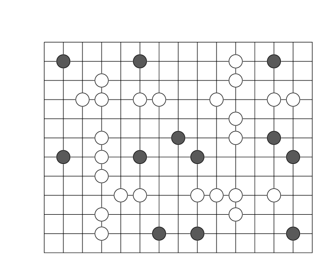
Figure 5: An example of a partially jammed configuration of the DRD model in two dimensions: atoms (denoted by white circles), on a finite number of horizontal or vertical lines can move, while all others (black circles) are completely immobile.

An unexpected offshoot of our study was the construction of an infinity of conservation laws for the special case of the $U=-1$ Bariev model, from the construction of the irreducible string. It would be interesting to see if similar constructs can be found for other quantum Hamiltonians, or for other stochastic evolution models having the MSD property.

References

- [1] M. Barma, M.D. Grynberg and R.B. Stinchcombe, Phys. Rev. Lett 70: 1033 (1993).
- [2] R.B. Stinchcombe, M.D. Grynberg and M. Barma, Phys. Rev. E 47 : 4018 (1993).
- [3] M. Barma and D. Dhar, Phys. Rev. Lett 73 : 2135 (1994).
- [4] M. Barma, in Nonequilibrium Statistical Mechanics in One Dimension, V. Privman ed., (Cambridge University Press, to appear).
- [5] M. Barma and D. Dhar, in Statphys-19 (The 19th IUPAP International Conference on Statistical Physics, Xiamen), (World Scientific, Singapore, p. 72, 1996).
- [6] D. Dhar and M. Barma, Pramana J. Phys. 41 : L193 (1993).
- [7] M. Barma and D. Dhar, in Proceedings of the International Colloqium on Modern Quantum Field Theory II, S.R. Das, G. Mandal, S. Mukhi and S.R. Wadia eds., (World Scientific, Singapore, 1995), p. 123.
- [8] This property implies that the stochastic transition matrix can be decomposed into a block diagonal form. This property has been called “complete reducibility” or “decomposability”. (See, e.g. N. G. van Kampen, Stochastic Processes in Physics and Chemistry, (North Holland, Amsterdam, 1981).) In a many-sector decomposable system, the number of such blocks is exponentially large.
- [9] R.Z. Bariev, J. Phys. A 24 L-549-533 (1991).
- [10] C. Boldrighini, G Cosimi, S. Frigio and M. Grasso Nunes, J. Stat. Phys.55 : 611, (1989).
- [11] B. Derrida, S. Janowsky, J.L. Lebowitz and E.R. Speer, J. Stat. Phys.76: 1153, (1994).
- [12] P.A. Ferrari, L.R.G. Fontes and Y. Kohayakawa., J. Stat. Phys. 76 : 813, (1993).
- [13] B. Schmittmann and R.K.P. Zia, in Phase Transitions and Critical Phenomena Vol 17 : eds. C. Domb and J.L. Lebowitz (Academic Press, New York, to appear).
- [14] See for example, Z.Q. Ma “Yang-Baxter Equation and Quantum enveloping algebras”, (World Scientific, Singapore, 1990). Chapter II.
- [15] F.C. Alcaraz, M. Droz, M. Henkel and V. Rittenberg, Annals. of Phy. 230: 250, (1994).
- [16] J.E. Hirsch, Phys. Lett. A 134, 451 (1989); Physica 158 C 326 (1989).
- [17] See, for example, the article by L.A. Takhtajan in Exactly Solvable Problems in Condensed Matter and Relativistic Field Theory, B.S. Shastry, S.S. Jha and V. Singh, eds. (Springer-Verlag, Berlin, 1986) pp. 175-219.
- [18] S.N. Majumdar and M. Barma, Physica A 177: 366 (1991).
- [19] M.K. Hari Menon and D. Dhar, J. Phys. A, 28, :6517, (1995).
- [20] M.K. Hari Menon, Ph.D thesis, Bombay University, (1995).
- [21] M. Kardar, G. Parisi and Y-C. Zhang, Phys. Rev. Lett 56 : 889, (1986)
- [22] J.P. Doherty, M.A. Moore, J.M. Kim and A.J. Bray, Phys. Rev. Lett. 72 : 2041, (1994).
- [23] M. Kardar and A. Zee., to appear in Nucl. Phys. B FS.
- [24] D. Dhar, Phase Transitions 9 : 51, (1987); L-H. Gwa and H. Spohn, Phys. Rev. A 46 : 844, (1992).
- [25] T. Halpin-Healy and Y-C. Zhang, Phys. Rep. 254 : 215, (1995).
- [26] D. Kim, Phys. Rev. E 52 : 3512, (1995).
- [27] R.J. Baxter, T.G. Enting and S.K. Tsang, J. Stat. Phys. 22 : 465, (1980).