[

AC Dynamics and Metastability of a Flux-Line Lattice

Abstract

We have measured the complex surface impedance of 2H-NbSe₂ in the mixed state over a wide range of magnetic field(0-2T) and frequency(10-3000MHz). A crossover between pinned and viscous dynamics of flux-lines is observed at a pinning frequency, $\omega_{p}$. The measured $\omega_{p}$ is compared to that predicted by a single-particle “washboard potential” model for the pinning interaction. When the flux lattice is prepared in an ordered state by zero-field cooling or by driving it with a large current, $\omega_{p}$ is in good agreement with the predicted value. However, when it is prepared in a metastable disordered state by field cooling, $\omega_{p}$ is nearly two orders of magnitude higher than expected indicating a complete break-down of the single-particle model.

] Pinning of the magnetic flux line lattice (FLL) due to material disorder plays an important role in the transport properties of type II superconductors[1]. It can lead to non-dissipative DC transport and to enhanced screening of electromagnetic fields. Most studies of pinning have focused on the DC critical current, $j_{c}$, at which the FLL breaks loose from the pinning centers and starts moving. However, the observation of phenomena such as current induced annealing[2, 3, 4, 5] and finite response times to large current pulses[4], have shown that the threshold measurements do not completely characterize the pinned state. A complementary approach is to probe the frequency dependence of the response to subcritical AC currents which induce small oscillations about the pinned state. This is described in a mean-field model [6, 7] by the equation of motion:

$$\eta\dot{u}+\kappa_{p}u=\Phi_{0}j(t)$$ (1)

where $j(t)=je^{-i\omega t}$ is the applied current density (in general, thermal driving forces can be included), $u$ is the displacement from equilibrium, $\kappa_{p}$ is a restoring force constant due to pinning, $\eta$ is the viscosity and $\Phi_{0}=\frac{hc}{2e}$ the flux quantum. At a characteristic pinning frequency, $\omega_{p}=\kappa_{p}/\eta$ there is a crossover from a low frequency regime where the FLL is pinned and the response non-dissipative to a high frequency regime of free flux motion with viscous response. Such a crossover was indeed observed in early AC resistivity measurements of alloy superconductors[6], but recent results in high $T_{c}$ samples were not compatible with mean-field behavior [8].

In this Letter we report on swept frequency measurements[9] (10-3000MHz) of the surface impedance in the mixed state of the low $T_{c}$ superconductor 2H-NbSe₂. The results are in good agreement with mean-field calculations of the electromagnetic response[7] which include contributions from Cooper pairs, the normal fluid, flux flow and pinning. A distinct crossover frequency is observed separating the regimes of pinned and viscous response. We find that $\omega_{p}$ exhibits a striking sensitivity to the state of the FLL: for the same field and temperature the FLL can have pinning frequencies which differ by as much as two orders of magnitude, depending on how the FLL is prepared. This surprising result is interpreted in light of pronounced metastability effects that were observed in DC and pulsed current measurements [4, 5]. If the FLL is prepared by zero field cooling to $T<T_{c}$ and then applying a field, H, the FLL enters one of two stable states. For (H,T) below a well-defined transition line, $T_{m}(H)$, which is marked by a jump in $j_{c}$, the state is ordered and weakly pinned, while above $T_{m}(H)$ it is more strongly pinned and disordered. However, cooling the FLL from above $T_{c}$ in a constant field always results in a disordered FLL. Below $T_{m}(H)$, the disordered FLL is metastable: it can be annealed into the ordered state by driving it with a current that exceeds $j_{c}$, by changing the field or by mechanical shock (after annealing $j_{c}$ is up to six times lower). The ordered state is stable against such variations. Our present results show the dramatic differences in the AC dynamics of the two states below $T_{m}(H)$: in the ordered state the FLL has a relatively low $\omega_{p}$ which is consistent with the measured $j_{c}$ in a single-particle washboard model. By contrast, in the metastable disordered state, $\omega_{p}$ is nearly two orders of magnitude higher than predicted by this model, indicating the existence of complex underlying dynamics.

The experimentally accessible quantity at high frequencies (where the AC fields are shielded out of bulk samples) is the surface impedance, $Z_{s}=R_{s}-iX_{s}$ [10]. $R_{s}$ and $X_{s}$ are the surface resistance and reactance. In the mixed state, $Z_{s}$ can be expressed in terms of a complex penetration depth, $\Lambda$, by $Z_{s}=-i\mu_{0}\omega\Lambda$. $\Lambda$ is determined by the response of Cooper pairs, the normal fluid and flux-lines[7]:

$$\Lambda=\left(\frac{\lambda^{2}+i\delta^{2}_{v}/2}{1-2i\lambda^{2}/\delta^{2}_{nf}}\right)^{1/2}.$$ (2)

Here $\lambda$ is the London penetration depth, $\delta_{nf}$ is the normal fluid skin depth, $\delta_{v}=(2\rho_{v}/\mu_{0}\omega)^{1/2}$ is the flux-line skin depth and $\rho_{v}$ is the flux-line resistivity. Our results are expressed in terms of the reduced variables, $r_{s}=R_{s}$(T)/$R_{s}$(T${}_{c})=Im(\frac{2\Lambda}{\delta_{n}}$) and $x_{s}=X_{s}$(T)/$X_{s}$(T${}_{c})=Re(\frac{2\Lambda}{\delta_{n}}$), which eliminate a trivial $\omega^{1/2}$ dependence, due to the skin effect. The normal state skin depth, $\delta_{n}$, is almost independent of H and T in our samples. This was determined from measurements of the normal state resistivity, $\rho_{n}$. Most results described here are in a range of H,T, and $\omega$ where $\lambda\ll\delta_{v},\delta_{nf}$ and the response is dominated by the flux-lines:

$$r_{s}-ix_{s}=(-2i\rho_{v}/\rho_{n})^{1/2}.$$ (3)

If we assume the Bardeen-Stephen value for the viscosity, $\eta=\Phi_{0}H_{c2}$/$\rho_{n}$, with $H_{c2}$ the upper critical field, then in the model described by (1), the flux-line resistivity is:

$$\rho_{v}(\omega)=\rho_{v1}(\omega)-i\rho_{v2}(\omega)=\frac{\omega^{2}-i\omega\omega_{p}}{\omega^{2}+\omega_{p}^{2}}\frac{H}{H_{c2}}\rho_{n}.$$ (4)

In the free flux flow limit ($\omega\gg\omega_{p}$), the response is further simplified and reduces to that of a normal metal with a purely real resistivity, $\rho_{n}H/H_{c2}(T)$:

$$\!r_{s}(T,H)\!=\!x_{s}(T,H)\!=\!\!\begin{array}[]{ll}(H/H_{c2}(T))^{\frac{1}{2}}&\quad\mbox{$T\leq T_{c}(H)$}\end{array}.$$ (5)

Measurements were done on two single crystal samples. For sample 1 ($\sim$2.5 x 2.5 x .1mm) $T_{c}=$ 7.2K, $\Delta T_{c}=$80mK, and the residual resistivity ratio, RRR=23. For sample 2 ($\sim$4 x 4 x .025mm) $T_{c}$ = 5.85K, $\Delta T_{c}$=80mK and RRR =9. The parameters indicate that sample 2 is relatively impure, and that both have good homogeneity. The field was along the sample’s c-axis, and the AC current was in the a-b plane. We will focus on data for sample 2.

The experimental setup [5] is shown in Fig. 1. The sample is mounted on a sapphire plate, which is attached to a stainless steel holder inside a vacuum can. A 50$\Omega$ coplanar transmission line consisting of three Cu strips (one central conductor between two ground planes) on an alumina substrate is placed close to the sample. The sample’s surface resistance (reactance) introduces a slight change ($\leq 10^{-4}$) in the magnitude (phase) of the signal propagating along the transmission line. This effect is isolated from a large background by modulating the sample temperature at a low frequency ($\sim$5-10Hz) with a resistive heater. The mixer puts out a signal at the modulation frequency, which is proportional to $cos(\phi)dR_{s}/dT+sin(\phi)dX_{s}/dT$, and is detected with a lock-in amplifier. By tuning $\phi$, the phase difference between the LO and RF ports, the derivative with respect to temperature of $R_{s}$ and $X_{s}$ can be measured separately. All the data were taken in the linear regime: the RF currents in the sample were $\sim$1mA ($j\sim 1A/cm^{2}\ll j_{c}$) and the amplitude of the flux-line motion ($<$.1Å at 10MHz) was negligible compared to their spacing.

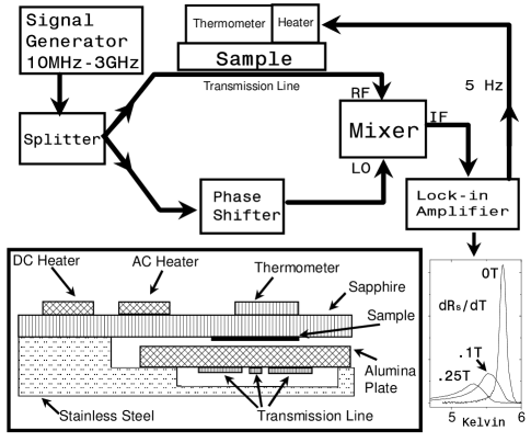
FIG. 1.: Upper Panel: schematic diagram of the measurement technique. Lower panel: cross sectional view of the sample holder and transmission line.

We first present the results in the disordered state. The FLL was prepared in this state by cooling from above $T_{c}$ to 3K in a constant field. In Fig. 2 we show the T dependence of $r_{s}$ and $x_{s}$. The data was obtained by slowly ramping T as $dR_{s}/dT$ or $dX_{s}/dT$ was measured. $r_{s}$ was obtained from the raw data in the following manner. The zero field data were integrated, with the integration constant fixed by assuming that $R_{s}$=0 for $T\ll T_{c}$. The integrated data were scaled to be equal to 1 at $T_{c}$. The value of the scaling factor depends on the coupling between sample and transmission line which is independent of H and therefore the same scaling factor was used for the finite field data. The finite field integration constants were set by using the fact that $Z_{s}$ is independent of field in the normal state. The same basic procedure was used for the reactance data, but determining the integration constants was complicated by the fact that even at low temperatures and zero field, $X_{s}$ has a finite value $\mu_{0}\omega\lambda$ and the absolute value of $\lambda$ was not measured directly. The necessary parameter $x_{0}\equiv x_{s}(3K,0T)=2\lambda(3K,0T)/\delta_{n}$, was determined by the method described below.

In Fig. 2a the measured $r_{s}(T)$ at 2.8 GHz is compared to the calculated values. For fields $\geq$.1T, the approximate expression (5) is in good agreement with the data. This calculation had no adjustable parameters since $H_{c2}(T)$ was obtained from DC measurements of $T_{c}(H)$. The agreement indicates that for this frequency the FLL is in the free flux flow regime and consequently the pinning frequency for the disordered state $\omega^{d}_{p}\ll$2.8GHz. At lower fields, $\delta_{v}\sim\lambda$ and the approximate expression is no longer adequate. Fitting the data at .01, .02, and .05T to the full expression (2), with $x_{0}$ as an adjustable parameter, we obtain $x_{0}\sim$.09 at 2.8GHz. This value was used to process the reactance data shown in Fig. 2b. We see that the full expression is in good agreement with the data at all fields for both $r_{s}$ and $x_{s}$. (A small contribution from pinning, determined by the measured pinning frequencies, was included in these calculations. At the higher fields, this is the main source of the slight difference between the calculations using (2) and (5)).

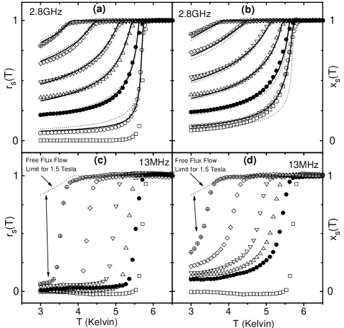
FIG. 2.: The temperature dependence of the surface resistance and surface reactance at 2.8GHz (a and b) and 13MHz (c and d) for 0 field ($\Box$), .02T ($\bigcirc$), .1T ($\bullet$), .25T ($\bigtriangleup$), .5T ($\bigtriangledown$), 1T ($\Diamond$), and 1.5T ($\otimes)$. The FLL was field cooled in all cases. The dotted lines were calculated using (5); the solid lines were calculated using (2). The double arrows show the deviation from free flux flow behavior.

Since $x_{0}=\frac{2\lambda(3K,0T)}{\delta_{n}}$ and $\delta_{n}$ depends only on $\rho_{n}$, which was measured, the value of $x_{0}$ can be used to determine $\lambda$. From the data at several frequencies in the GHz range, we estimate $\lambda\sim$1200-1400Å in sample 2 and $\sim$1000-1200Å in sample 1. Previous estimates are scattered over the range 700-2500Å [11].

In Figs. 2c and 2d we show the results at 13MHz. In this case, both $r_{s}$ and $x_{s}$ are well below the free flux flow values, indicating that $\omega^{d}_{p}>13$MHz. The frequency dependence of the response over the entire range, shown in Fig. 3, exhibits a crossover from pinned to free behavior. The best fit of the data to (3), with $\rho_{v}$ given by (4), is obtained for $\omega^{d}_{p}=125$MHz. The upper inset of Fig. 3a, shows the temperature dependence of $\omega^{d}_{p}$ and $j_{c}$ at .5 T. The lower insets in Fig. 3 show that the data for all fields collapse when plotted as a function of $\omega/\omega^{d}_{p}(T,H).$ This universal behavior demonstrates that in this state the frequency dependence of the response of the FLL is completely characterized by one parameter, $\omega^{d}_{p}$, as expected from (1).

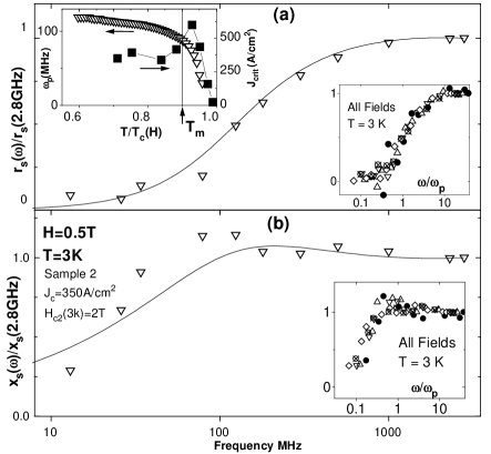
FIG. 3.: The frequency dependence of $R_{s}$ (a) and $X_{s}$ (b) at 3K and 0.5T. (a), upper inset: field and temperature dependence of the pinning frequency. Lower insets: the collapse of the data for all fields. Symbols are the same as in Fig. 2.

We now turn to the response in the ordered state. When the FLL is prepared in this state and then heated above $T_{m}$, it undergoes an order to disorder transition that is irreversible in temperature [4]. Thus, $dR_{s}/dT$ and $dX_{s}/dT$ cannot be obtained with this technique over the entire temperature range and it is not possible to set the integration constants (since this requires data up to $T_{c}$). Although the absolute values of $r_{s}$ and $x_{s}$ cannot be determined, the relative changes, $\Delta r_{s}(T)$ and $\Delta x_{s}(T)$, are still accessible for $T<T_{m}$. At frequencies in the GHz range, the results are independent of how the FLL is prepared. In Fig. 4a, we plot $\Delta r_{s}(T)$ at 13MHz in both states. The data in the disordered state is essentially constant in temperature, consistent with the high pinning frequency of this state. In the ordered state however the data has a substantial slope which is close to its value at 2.8GHz, indicating that the pinning frequency in this state $\omega^{o}_{p}<$13MHz.

Since the value of $\omega^{o}_{p}$ appears to be in the MHz range, it can be measured by more conventional means. At these frequencies the sample thickness is much less than $\delta_{v}$, so that the skin effect is negligible and $\rho_{v}$ could be accessed directly with a 4-lead technique. The sample used for these measurements was from the same batch as sample 2 and had nearly identical parameters. A background signal was determined from zero field measurements at $T\ll T_{c}$ and subtracted from the data. In Fig. 4b we see that in the disordered state both $\rho_{v1}$ and $\rho_{v2}$ are vanishingly small over the entire frequency range, 0-200kHz, indicating that $\omega^{d}_{p}\gg$200kHz, in accord with the previous result. By contrast, $\rho_{v1}$ and $\rho_{v2}$ are finite in the ordered state and their frequency dependence gives , $\omega^{o}_{p}\sim$1MHz.

To interpret the results, we use a model where the FLL is treated as a single particle moving in a washboard potential: $V(u)=V_{0}(1-cos(\frac{2\pi u}{r_{p}}))$. $u$ is the displacement from equilibrium and $r_{p}$ is a characteristic length scale for the interaction of the FLL with the pinning sites. In this model, the critical current is $j_{c}=\frac{2\pi V_{0}}{r_{p}\Phi_{0}}$ and the restoring force constant is $\kappa_{p}=V_{0}(\frac{2\pi}{r_{p}})^{2}=j_{c}\frac{2\pi\Phi_{o}}{r_{p}}$ leading to:

$$\omega_{p}=\frac{\kappa_{p}}{\eta}=\frac{2\pi}{r_{p}}\frac{j_{c}\rho_{n}}{H_{c2}}.$$ (6)

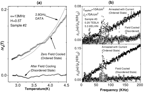
FIG. 4.: Comparisons of the AC response for the disordered and ordered states below $T_{m}$ (a) $\Delta r_{s}(T)$ at 13MHz. (b) The frequency dependence of the complex resistivity. The noise near 75KHz is instrumental.

For the ordered state data shown in Fig. 4b, $j_{c}$ = 70A/cm². Choosing $r_{p}$=$a_{0}$ (where $a_{0}\cong(\Phi_{0}/H)^{1/2}$ is the flux line spacing), as is usually done, gives $\omega^{o}_{p}$=1.4 MHz, in rough agreement with the data. In the disordered state ($j_{c}(3K,0.5T)$= 350A/cm²), the washboard model gives $\omega_{p}$= 2.6 MHz, which is 45 times lower than the observed value. This discrepancy is similar everywhere in the H-T plane except above T${}_{m}(H)$ (where the disordered state is stable), in which case it is much smaller. The washboard model can give a higher $\omega_{p}$ if $r_{p}$ is reduced. But even using the smallest length scale in the problem, the coherence length, and taking into account the structure of the flux-line core[1] leads to values that are not much larger: $\omega_{p}$(3K,.5 T)=4.7 MHz. In addition, the washboard model cannot account for the qualitative difference in the temperature dependences of $\omega_{p}$ and $j_{c}$. Thus, this model successfully describes the connection between $j_{c}$ and $\omega_{p}$ in the ordered state, but fails to do so in the metastable disordered state. This is due to the single particle treatment of the FLL in which both $j_{c}$ and $\omega_{p}$ are determined by the shape of a pinning potential. In this model, $j_{c}$ is the current to drive the entire FLL out of a potential. However, the metastable state reorders as it depins and $j_{c}$ for this state may actually be the current at which the FLL becomes unstable to rearrangements which create continuous channels of mobile flux lines. Evidence for channel formation and growth was previously observed with DC[4, 5, 12] and pulsed current measurements[4], as well as in computer simulations[13]. However, in the AC measurements, no rearrangements can take place because of the low driving currents and the short time scales.

In summary, the AC response in both states exhibits a crossover between pinned and free behavior which can be described by a simple equation of motion. In the ordered state the connection between $\omega_{p}$ and $j_{c}$ is accurately predicted by a single particle washboard model, but for the metastable disordered state the model breaks down. The two states discussed here are possible candidates for the proposed vortex glass (disordered) and pinned lattice or Bragg glass (ordered)[14]. Our results indicate that each of these states can be supercooled or superheated across T_m into the stability region of the other[4, 5]. In this picture, the metastable disordered state corresponds to a supercooled vortex glass.

We thank N. Andrei, D.A. Huse and R. Walstedt for useful comments. Supported by NSF-DMR-9401561.

REFERENCES

- [1] G. Blatter et al. Rev. Mod. Phys., 66, 1125 (1994)
- [2] R. Wördenweber, P. H. Kes, and C. C. Tsuei Phys. Rev. B, 33, 3172 (1986).
- [3] U. Yaron et al., Phys. Rev. Lett. 73, 2748 (1994)
- [4] W. Henderson, E.Y. Andrei, M.J. Higgins, and S. Bhattacharya , Phys. Rev. Lett. 77, 2077 (1996)
- [5] W. Henderson, Rutgers University PhD Thesis (1996).
- [6] J. Gittleman and B. Rosenblum, Phys. Rev. Lett., 16, 734 (1966)
- [7] M. Coffey and J. Clem, Phys. Rev. Lett., 67, 386 (1991); Phys. Rev. B, 46, 11757 (1992); E. Brandt, Physica C, 185-189 270 (1991); C.J. van der Beek, V.B. Geshkenbein, V.M. Vinokur, Phys. Rev. B, 48, 3393 (1993)
- [8] H. K. Olsson et al., Phys. Rev. Lett. 66, 2661 (1991); H. Wu, N.P. Ong, and Y.Q. Li, Phys. Rev. Lett., 71, 2642 (1993); Y. Ando et al., Phys. Rev. B 50, 9680 (1994); D. Wu, J.C. Booth, and S. Anlage, Phys. Rev. Lett., 75, 525 (1995)
- [9] E.Y. Andrei, S. Yucel and L. Menna, Phys. Rev. Lett. 67, 3704 (1991).
- [10] C. Kittel, Quantum Theory of Solids, John Wiley and Sons, New York (1987)
- [11] P. de Trey et al., J. Low Temp. Phys. 11, 1973; R.E. Schwall et al., J. Low Temp. Phys. 22 557 (1976); K. Takita et al., J. Low Temp. Phys. 58, 127 (1985); L.P. Le et al., Physica C, 185-189, 2715 (1991)
- [12] M. Hellerqvist et al., Phys. Rev. Lett. 76, 4022 (1996)
- [13] H. J. Jensen, A. Brass, and A. J. Berlinsky, Phys. Rev. Lett. 60, 1676 (1988); N. Grnbech-Jensen, A. R. Bishop, and D. Domínguez, Phys. Rev. Lett. 76, 2985 (1996); C. Reichhardt et al., Phys. Rev. B 53, R8898 (1996)
- [14] M.J.P. Gingras and D.A. Huse, Phys. Rev. B 53, 15193 (1996); T. Giamarchi and P. Le Doussal, Phys. Rev. Lett. 74, 606 (1995)