and

Lacunarity of Random Fractals

Abstract

We discuss properties of random fractals by means of a set of numbers that characterize their universal properties. This set is the generalized singularity spectrum that consists of the usual spectrum of multifractal dimensions and the associated complex analogs. Furthermore, non-universal properties are recovered from the study of a series of functions which are generalizations of the so-called energy integral.

A number of the properties of fractals are associated with their Hausdorff, box-counting, or fractal dimensions. But further information of a universal character is also encoded in secondary (singular) dimensions, some of which may be complex. For example, a recurrent theme in the study of fractals is that of asymptotic or logarithmic periodicity [1, 2]. Most fractal objects and mathematical constructions thereof are not exactly scale invariant. Rather, they obey simple recurrence relations that relate an infinite but discrete set of scales. Recent physical examples include the appearance of complex exponents in diffusion-limited aggregation [3], crack propagation in two dimensions [4], and Boolean delay equations in the modelling of climate dynamics [5].

For instance, instead of the full scale invariance of a function of local variables,

$$F(x)=\lambda^{D}F(x/\lambda),$$ (1)

we have the logarithmic analog of Bloch’s theorem,

$$F(x)=\lambda^{D}F(x/\lambda)\,G(\ln\lambda),$$ (2)

where $G$ may be a periodic function.

This is a rather well-known relation but we feel that it has been under exploited. The period of $G$ is independent of the scaling dimension, $D$, and gives further information of the properties of the fractal object.

The ways in which the fractal dimensions of the object manifest itself are manifold. Consider, in particular, a set of analytical quantities calculated from the real space distribution of a fractal object, namely, the set of correlation integrals:

$$C_{q}(r)=\int d\mu(x)\left(\int d\mu(y)\,\,\theta(r-|x-y|)\right)^{q-1},$$ (3)

where $q\geq 2$, $\theta$ is the Heaviside step function, and $d\mu$ is the measure of the object in question. The scaling properties of these correlation integrals with respect to the distance $r$ define a countable set of dimensions forming part of the multifractal dimension spectrum [6, 7, 8].

The study of the scaling properties of such correlations is facilitated by considering the corresponding energy integrals:

$$I_{q}(\tau)=\int r^{-\tau}\,dC_{q}(r),\quad\tau<d,$$ (4)

where $\tau$ is restricted to be less than the spatial dimension, $d$. Note that $I_{q}(\tau)$ is related to the Mellin transform of $C_{q}(r)$ [9].

At this point the spatial information of the fractal has been encoded in these energy integrals, which are typically, but not always, meromorphic. For particular cases of deterministic Cantor sets, it is shown in [10, 11] that the complex structure of these functions (4) reveal singularities that correspond to the relevant scaling dimensions of the theory. One usually one keeps only the most relevant, i.e., the one with the smallest real part, but the rest of the spectrum is important in studying finite-size effects.

More precisely, the most relevant singularity is a pole on the real axis and has a numerical value that is a lower bound to the Hausdorff dimension. This was first proved by Frostman for $q=2$ [12] (see also Falconer [13]). In some cases, the Hausdorff dimension also corresponds to the box-counting dimension [13, 14].

Typically, the rest of the singularities are also poles, and appear as pairs of complex conjugates with real parts not smaller than the Hausdorff dimension. The imaginary parts of these poles correspond obviously to the logarithmic wavelength of the fractal, while the residues appear as the amplitudes of oscillations observed in the asymptotic scaling of various correlation integrals (3). This program of the analysis of a fractal object has been carried out, albeit in a somewhat scattered way, for the middle-third Cantor set and some of its deterministic generalizations [10, 11, 15]. This complex singularity spectrum has been called the multilacunarity spectrum [11]. It is the goal of our work to show that it is well-defined for classes of random fractals, and we explicitly compute the lacunarity of a particular example.

It turns out that for some simple but important examples the Hausdorff dimension is easy to calculate with the use of a little ingenuity. Just as simply, the satellite dimensions can be calculated in the same way without resorting to the explicit computation of the correlation integrals (3) or the energy integrals (4).

For the middle-third Cantor set, and for many other objects with simple recursive descriptions, we consider an equation that relates the relative scales, $\ell_{i}$, and the relative (normalized) measures, $p_{i}$, at successive levels of approximation,

$$\sum_{i}\frac{p_{i}^{q}}{\ell_{i}^{\tau}}=1.$$ (5)

In the case of the middle-third Cantor set, $\ell_{i=1,2}=1/3$ and $p_{i=1,2}=1/2$, and (5) becomes $2^{q-1}/{3^{\tau}}=1$. The unique real solution, $\tau(q)=(q-1)\ln 2/\ln 3$, gives the Hausdorff dimension. In general, $\tau=\tau(q)$ is not linear in $q-1$ and gives one the desired multifractal dimension spectrum via the relation $D_{q}=\tau(q)/(q-1)$. In this way, the universal properties of the fractal, namely, its generalized dimensions, are rather easily computed [7, 16].

However, as noticed in [11], a study of the middle-third Cantor set (and some deterministic generalizations), (5) also has complex roots. For instance, in the case of the middle-third Cantor set,

$$\tau(q)=(q-1)\frac{\ln 2}{\ln 3}+i\frac{2\pi j}{\ln 3},\,\,j=0,\pm 1,\pm 2,\ldots$$ (6)

The imaginary parts of these complex roots correspond to the period of $G$ in (2) and the logarithmic period observed in the correlation integrals [2].

The reason for the surprising success of this approach, which reduces the sometimes formidable calculation of the energy integrals (4) to the computation of a partition function (5), is that one has implicitly utilized the recursive structure of the fractal distribution [encoded as (2)]. In doing so, one successfully captures the fact that the fractal has a very well defined set of real-space singularities, and equates the determination of the spectrum of the many-body problem to the solution of a relatively simple transcendental equation.

So far we have examined results for deterministic fractals, where the scale invariance of (2) is exactly satisfied. Consider now the case in which the fractal is not exactly self-similar, but is only statistically self-similar, i.e., scaling functions obey (2) only on average. We shall make precise what this averaging procedure entails (for related issues of averaging of stochastic hierarchical processes, see [17]).

For a process that generates a generalized Cantor set by replacing each segment at level $l$ by $m$ segments at level $l+1$, we let the length of the segments, $\ell_{i}(i=1,\ldots,m)$, be random variables with random probability measures $p_{i}(i=1,\ldots,m)$. For this and other random fractals, we define a new set of correlation integrals as the expectations of (3), given a probability distribution of the $p_{i}$’s and the $\ell_{i}$’s:

$${\mathcal{C}}_{q}(r)=E\left[C_{q}(r)\right],$$ (7)

where $E$ denotes expectation and $C_{q}(r)$ is the value of the correlation integral for a single realization of the random fractal. A new energy integral may be defined in precisely the same fashion:

$${\mathcal{I}}_{q}(\tau)=E\left[I_{q}(\tau)\right],\quad\tau<d.$$ (8)

It has been shown by Falconer [18] that the probabilistic version of equation (5) still gives the relevant dimension spectrum, i.e, one has to solve the expectation equation,

$$E\left[\sum_{i=1}^{m}\frac{p_{i}^{q}}{\ell_{i}^{\tau}}\right]=1,$$ (9)

to obtain the multifractal dimension spectrum.

The conditions for the existence of a unique and meaningful real solution of (9) have been studied [18, 19, 20], and simple extensions of these considerations lead to the existence of well-defined complex solutions in complete analogy with the deterministic case.

Consider then the following example of a randomized Cantor set. At level $l$ of the recursive construction, we divide each segment into $n$ equal segments and pick $m$ of them at random with uniform probability. We assign to each of the $m$ smaller segments a measure $1/m$-th of the original segment. To simplify the presentation, we examine only the case for $q=2$ and do not consider the more general model of Falconer [18], which involves possibly non-uniform probability distributions $p_{i}$ and $\ell_{i}$. However, the computation may be generalized for higher-order correlation integrals and for non-uniform probability distributions satisfying the restrictions outlined in [18].

At level $l$ of this process, the energy integral is simply related to the energy integral of the previous level:

$${\mathcal{I}}^{(l)}(\tau)=mn^{-\tau}\,{\mathcal{I}}^{(l-1)}(\tau)+{\mathcal{R}}(m,n,\tau),$$ (10)

where the superscripts denote the finite-level approximation of the energy integral. The function ${\mathcal{R}}$ is given by

$${\mathcal{R}}(m,n,\tau)=\frac{2n(m-1)(1-n^{\tau-2})}{m(n-1)(\tau-1)(\tau-2)}.$$ (11)

Explicit derivation of ${\mathcal{R}}$ for this example is given as an appendix. Note that in (10), the prefactor $mn^{-\tau}$ is the expected value of the partition function for this model. So that the energy integral of the limiting distribution is simply

$${\mathcal{I}}(\tau)=\frac{{\mathcal{R}}(m,n,\tau)}{1-mn^{-\tau}}\,.$$ (12)

All of the singularities of ${\mathcal{I}}(\tau)$ are given by the zeros of the denominator on the right-hand side of (12),

$$mn^{-\tau}=1,$$ (13)

as expected. It is easily checked that (11) is not singular at $\tau=1$.

The roots of (13) are at

$$\tau_{j}=\frac{\ln m}{\ln n}+i\frac{2\pi j}{\ln n}\,,\quad j=0,\pm 1,\pm 2,\ldots$$ (14)

Thus, we expect the correlation integral to exhibit oscillations of period $\ln n$. By using properties of inverse Mellin transforms [9], the correlation integral can be written as

$${\mathcal{C}}(r)=r^{D}\left(\frac{\alpha_{0}}{\tau_{0}}+2\sum_{j=1}^{\infty}\left|\frac{\alpha_{j}e^{i\phi_{j}}}{\tau_{j}}\right|\cos\left(2\pi j\frac{\ln r}{\ln n}-\phi_{j}\right)\right),$$ (15)

where $D=\ln m/\ln n$ is the (second-order) correlation dimension. $\alpha_{j}$ and $\phi_{j}$ are real and are determined by the residues at $\tau_{j}$ (for $j$ non-negative): The residue at the $j$-th pole is of the form, $\alpha_{j}\exp(i\phi_{j})$. We propose to call the modulus of $\alpha_{j}e^{i\phi}/\tau_{j}$ (and the higher-order analogs) the lacunary amplitudes.

In Fig. 1, we compare the expected scaling of the correlation integral with an ensemble average of the scaling for the case $n=3$ and $m=2$. The average is performed over several (in this case, twelve) numerical realizations of the random fractal (approximated at level $l=15$). We plot the residuals, $r^{-\ln m/\ln n}{\mathcal{C}}(r)$, versus $r$. The dashed line is the ensemble average, and the solid line exhibits the expected oscillations of (15).

Figure 1: Log-log plot of $r^{-D}{\mathcal{C}}(r)$ versus $r$. Dotted curve is an ensemble average; solid curve is the expectation.

While it may seem superfluous to obtain the correlation integral from numerical computations once it has been calculated analytically, this exercise was interesting since we have not performed the average over a large ensemble. Rather we took the spatial average of a few instances of a random process. That both results were essentially the same over a number of logarithmic periods is a rather natural self-averaging property of many fractal objects. The fluctuation of the ensemble average about the expectation may be described by higher-order correlation integrals and will be discussed in a forthcoming publication [21]. In the present case, the small size of the ensemble produces disagreement with predictions at $r$ of the order of the system size. Furthermore, numerical resolution affects the correlation for $r$ smaller than $e^{-13}$.

We note that the measurement of the lacunarity spectrum is accessible using a variety of correlations. For instance, we may identify these complex dimensions in the logarithmically periodic oscillation of the Fourier transform [22] and the diffraction spectrum [22, 23]. However, while the same logarithmic periods are observed, the shape and phase of the oscillations vary. The periods arise from the additional discrete scale invariance of the underlying model and the numerical value of these periods are determined by the solutions of (9). The different measures of correlation (Fourier or Mellin transforms) reveal differently-valued residues located at the roots of (9).

Previous studies of the inverse fractal problem, i.e., the extraction of the (possibly stochastic) hierarchical process from the observed multifractal dimension spectrum, revealed ambiguities in the standard procedure: Namely, many models can be made to fit a given multifractal dimension spectrum [16, 24]. The approach described above provides the maximal characterization of the underlying multiplicative process without additional dynamical information. In this way, we may further distinguish between different hierarchical processes that give rise to fractals with similar dimension spectra (see also [17]).

We have to stress that the lacunarity spectrum does not resolve all the inherent ambiguities. Many models, random or deterministic, can be made to fit a given lacunarity spectrum. However, using the lacunarity spectrum, we may distinguish between processes that have the same multifractal dimension spectrum. What the lacunarity spectrum reveals is the possible additional discrete scale invariance which are not furnished by the previous attempts to characterize fractal systems. Furthermore, non-universal information is recovered from studying correlations (3) and energies (4).

How does this work bear on fractal sets generated by low-order (deterministic or stochastic) dynamical systems? Preliminary work [21] suggests that the complex solutions of the Lyapunov partition function (a dynamical analog of (5) and (9), see [25]) describes the anomalous scaling observed in simulations (see, for instance, [1]). In addition, the fact that the lacunarity spectrum can be calculated from a partition function (5) immediately implies that periodic orbit expansions [26] can be used to calculate the spectrum.

As for fractals generated by systems governed by large numbers of degrees of freedom (as featured most prominently in phenomena modeled by diffusion limited aggregation and in inhomogeneities of highly turbulent flows), this generalized multifractal description complements the traditional views. Studies thus far have taken the position that the deviations from strict power-law scaling are anomalous and, hence, have focused on establishing possible causes for this apparent deviation (an example being inertial range intermittency [8, 27] in turbulent fluids). In our approach, log-periodic deviations may be accommodated rather naturally (see also [2, 28]). Future efforts will be directed towards the description of turbulent intermittency using the analysis followed in this paper.

We gratefully acknowledge J. Fournier, R. Rosner, A. Sornborger, and E. Spiegel for helpful conversations. We thank R. Ball for bringing his work with R. Blumenfeld to our attention. We also wish to thank the anonymous referee for useful suggestions. This work was completed while F. J. S. was a Rosenbaum fellow at the Newton Institute. L. T. is supported by the U. K. Particle Physics and Astronomy Research Council.

Appendix

In this Appendix we present the details leading to the explicit formulas of the energy integral as given by (11) and (12).

We need to consider first the behavior of the measure upon averaging. Since we have assigned an equal probability to every possible case of segmentation, the expectation value for the density, $\rho(x)dx=d\mu(x)$, is uniform, i.e.,

$$E\left[\rho(x)\right]=1.$$ (A1)

To be able to perform the required multiple integrals, we need to evaluate the expectation of products of densities. Sufficient information about the joint distribution of these densities is obtained by considering one step in the recursive construction. After one such step, the interval $L^{0}=[0,1]$ is divided into $n$ subintervals $L^{1}_{i},i=1,2,\ldots,n$ from which $m$ subintervals will be chosen randomly. The set of all points $(x,y)$ that belong to the subintervals $L^{1}_{i}$ and $L^{1}_{j}$, respectively, form a square of size $n^{-1}\times n^{-1}$ in the $x$-$y$ plane. Such a square will be labelled $(i,j)$, as shown in Figure 2. The shaded region $R$ corresponds to those cases in which $x$ and $y$ are in disjoint intervals, i.e., $i\neq j$.

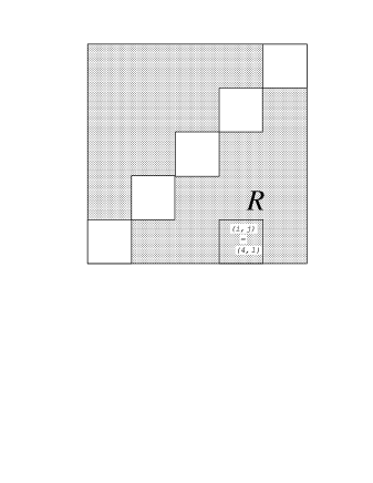
Figure 2: Different regions of integration for the energy integral (10). Shaded regions (labelled by $R$) contribute to the function ${\mathcal{R}}(m,n,\tau)$; white regions contribute to ${\mathcal{I}}^{(l)}(\tau)$. Labels of individual squares, $(i,j)$, are explained in the text. Shown here is a case for $n=5$.

Consider now one of the shaded squares, say $(i,j)$. The probability that the intervals $L^{1}_{i}$ and $L^{1}_{j}$ are indeed chosen is simply ${n-2\choose m-2}/{n\choose m}$. In this case, each of the intervals will support a measure of total mass $1/m$. Furthermore, since segmentation for each of these intervals proceeds uncorrelated, we have

$$E\left[\rho(x)\rho(y)\right] = \frac{{n-2\choose m-2}}{{n\choose m}}E_{i}\left[\rho(x)\right]E_{j}\left[\rho(y)\right]$$ (A2)

$$= \frac{m(m-1)}{n(n-1)}\frac{n^{2}}{m^{2}},\quad(x,y)\in(i,j),$$

where $E_{k}$ denote expectation conditioned to the event that segment $k$ is indeed chosen.

Next, we consider the diagonal squares. These squares will contribute to the energy integral with probability ${n-1\choose m-1}/{n\choose m}=m/n$. The process of segmentation for a subinterval is identical to that of the original interval. Therefore, if $L^{1}_{i}$ is chosen, the average of the product of densities $\rho(x)\rho(y)$ restricted to this interval is identical to that of the original interval up to rescaling. The rescaling matches $x$ from the $L^{1}_{i}$ segment with the point $x^{\prime}=nx-i-1$ in $L^{0}$. We have, for $x,y\in L^{1}_{i}$,

$$E\left[\rho(x)\rho(y)\right] = (m/n)E_{i}\left[\rho(x)\rho(y)\right]$$ (A3)

$$= (m/n)(1/m)^{2}E\left[\rho(x^{\prime})\rho(y^{\prime})\right]$$

Note also that $|x-y|=(1/n)|x^{\prime}-y^{\prime}|$. Thus the contribution to the energy integral from each of the diagonal squares is proportional to the overall expectation of the energy integral

$$E\left[\int_{(i,i)}\frac{d\mu(x)d\mu(y)}{|x-y|^{\tau}}\right]=(m/n)(1/m)^{2}n^{\tau}\,{{\mathcal{I}}}_{2}(\tau)$$ (A4)

Summing over all squares we obtain relation (10) where ${{\mathcal{R}}}(m,n,\tau)$ can now be identified with the expectation value of the energy integral restricted to the shaded region.

To simplify the calculation of ${{\mathcal{R}}}(m,n,\tau)$ we note that

$$E\left[\int_{R}\frac{d\mu(x)d\mu(y)}{|x-y|^{\tau}}\right]=\frac{m(m-1)}{n(n-1)}\left(\frac{n}{m}\right)^{2}\int_{R}\,\frac{dxdy}{|x-y|^{\tau}}$$ (A5)

Furthermore, the last integral satifies

$$\int_{0}^{1}\int_{0}^{1}\,\frac{dxdy}{|x-y|^{\tau}}=\int_{R}\,\frac{dxdy}{|x-y|^{\tau}}+n^{s-1}\int_{0}^{1}\int_{0}^{1}\,\frac{dxdy}{|x-y|^{\tau}}$$ (A6)

which readily gives the final result

$$R(m,n,\tau)=\frac{2n(m-1)(1-n^{\tau-2})}{m(n-1)(\tau-1)(\tau-2)}.$$ (A7)

References

- [1] R. Badii and A. Politi, Phys. Lett. A 104 (1984) 303.
- [2] L. A. Smith, J.-D. Fournier, and E. A. Spiegel, Phys. Lett. A 114 (1986) 465.
- [3] D. Sornette, A. Johansen, A. Arneodo, J. F. Muzy, and H. Saleur, Phys. Rev. Lett. 76 (1996) 251; H. Saleur and D. Sornette, J. Physique I 6 (1996) 327.
- [4] R. C. Ball and R. Blumenfeld, Phys. Rev. Lett. 68 (1992) 2254.
- [5] A. P. Mullhaupt, Phys. Lett. A 122 (1987) 403; Phys. Lett. A 124 (1987) 151.
- [6] P. Grassberger and I. Procaccia, Phys. Rev. Lett. 50 (1983) 346; H. G. E. Hentschel and I. Procaccia, Physica D 8 (1983) 435; P. Grassberger and I. Procaccia, Physica D 9 (1983) 189.
- [7] T. C. Halsey, M. H. Jensen, L. P. Kadanoff, I. Procaccia, B. I. Shraiman, Phys. Rev. A 33 (1986) 1141.
- [8] G. Paladin and A. Vulpiani, Phys. Rep. 156 (1987) 147.
- [9] A. Erdélyi (ed.), Tables of Integral Transforms (McGraw Hill, New York, 1954).
- [10] D. Bessis, G. Servizi, G. Turchetti and S. Vaienti, Phys. Lett. A 119 (1987) 345; D. Bessis, J.-D. Fournier, G. Servizi, G. Turchetti and S. Vaienti, Phys. Rev. A 36 (1987) 920.
- [11] J.-D. Fournier, G. Turchetti and S. Vaienti, Phys. Lett. A 140 (1989) 331.
- [12] O. Frostman, Meddel. Lunds Univ. Math. Sem. 3 (1935) 1.
- [13] K. J. Falconer, The Geometry of Fractal Sets (Cambridge University Press, Cambridge, 1985); Fractal Geometry: Mathematical Foundations and and Applications (John Wiley & Sons, New York, 1990).
- [14] R. Mainieri, CHAOS 3 (1993) 119.
- [15] E. Orlandini, G. Servizi, M. C. Tesi, and G. Turchetti, Nuovo Cimento B 106 (1991) 1221; E. Orlandini, M. C. Tesi, and G. Turchetti, J. Stat. Phys. 66 (1992) 515.
- [16] M. J. Feigenbaum, J. Stat. Phys. 46 (1987) 919; J. Stat. Phys. 46 (1987) 925.
- [17] H. G. E. Hentschel, Phys. Rev. E 50 (1994) 243.
- [18] K. J. Falconer, J. Theoret. Prob. 7 (1994) 681.
- [19] R. D. Mauldin and S. C. Williams, Trans. Am. Math. Soc. 295 (1986) 325; S. Graf, Prob. Theory Relat. Fields 74 (1987) 357; R. D. Mauldin, S. Graf, and S. C. Williams Proc. Natl. Acad. Sci. 84 (1987) 3959.
- [20] K. J. Falconer, Math. Proc. Camb. Phil. Soc. 100 (1986) 559; Proc. Amer. Math. Soc. 101 (1987) 337.
- [21] F. J. Solis and L. Tao (unpublished).
- [22] R. S. Strichartz, Trans. Amer. Math. Soc. 336 (1993) 335; C. P. Dettmann and N. E. Frankel, J. Phys. A 26 (1993) 1009; C. P. Dettmann, N. E. Frankel, and T. Taucher, Phys. Rev. E 49 (1994) 3171.
- [23] C. Allain and M. Cloitre, Phys. Rev. A 36 (1987) 5751; D. A. Hamburger, Phys. Rev. E (to be published).
- [24] A. B. Chhabra, R. V. Jensen, and K. R. Sreenivasan, Phys. Rev. A 40 (1989) 4593.
- [25] E. Ott, T. Sauer, and J. A. Yorke, Phys. Rev. A 39 (1989) 4212.
- [26] R. Artuso, E. Aurell, and P. Cvitanović, Nonlinearity 3 (1990) 325; Nonlinearity 3 (1990) 361.
- [27] U. Frisch, Turbulence: the Legacy of A.N. Kolmogorov (Cambridge University Press, Cambridge, 1995).
- [28] E. A. Novikov, Phys. Fluids A 2 (1990) 814.