Universal Phase Diagram for Vortex States of Layered Superconductors in Strong Magnetic Fields

Abstract

We report on a Monte Carlo study of the lowest-Landau-level limit of the Lawrence-Doniach model for a layered superconductor. We have studied order parameter correlation functions for indications of the broken translational symmetry and the off-diagonal long range order present in the mean-field-theory vortex lattice. Our results are consistent with a single first order phase transition between a low temperature 3D vortex solid phase, with both broken translational symmetry and off-diagonal long range order, and a high temperature vortex liquid phase with no broken symmetries. We construct a universal phase diagram in terms of dimensionless parameters characterizing intra-layer and inter-layer couplings. The universal phase boundary extracted from our simulations and the associated latent heats and magnetization jumps are compared with experiment and with numerical results obtained for related models.

I Introduction

Because of the combination of high transition temperature, strong planar anisotropy, and short coherence length that occurs in high temperature superconductors, strong thermal fluctuations are present over a wide temperature interval in these materials. Thermal fluctuations are especially important in a magnetic field where they are responsible for the melting of the Abrikosov[1] vortex lattice, often at temperatures that are well below the mean-field critical temperature, giving rise to a vortex liquid state [2, 3, 4, 5, 6, 7, 8, 9, 10] that is strongly diamagnetic but also strongly resistive. In this paper[11] we report on a Monte Carlo study of thermal fluctuations in layered superconductors with a magnetic field oriented perpendicular to the planes. Our study is based on a Lawrence-Doniach model[12] and employs the lowest-Landau-level (LLL) approximation[13, 14, 15] which is valid near the mean-field-transition temperature. The emphasis is on generic properties of this model rather than on quantitative estimates of phase diagrams, latent heats, and magnetization discontinuities for particular materials.[16] We find that, for this model, a single first order phase transition occurs between a low-temperature state and a high temperature state with no broken symmetries. The low temperature state has off-diagonal long-range-order (ODLRO) both along and perpendicular to the field direction and broken translational symmetry.

At the mean-field level, the phase transition between the normal state and the Abrikosov lattice state is highly unusual in two related respects. Firstly, the eigenvalue of the Cooper-pair density matrix which diverges at the transition point has a macroscopic degeneracy, in contrast to the isolated divergent eigenvalue with a zero-momentum-state eigenfunction found at zero magnetic field. The many divergent eigenvalues are associated with the many states in the Landau levels[17] into which the transverse translational degrees of freedom of the Cooper pairs are quantized. At the mean-field level, this unusual property is responsible for the simultaneous development of superconducting order and broken translational symmetry in the Abrikosov vortex lattice state. Another consequence is that, at temperatures well above the mean-field transition temperature $T_{c}^{MF}$, fluctuations in a magnetic field in $D$-dimensions are like those of a $D-2$ dimensional system[18] at zero magnetic field. Brézin et al.[19] first suggested, on the basis of expansions around the upper critical dimension for this problem ($D=6$), that fluctuations would drive the Abrikosov transition first order. Indeed Hetzel et al.[20] some time ago found evidence from Monte Carlo simulations that the transition is first order for $D=3$. This conclusion has been substantiated by a large volume of subsequent[21] work from various points of view, although there is not yet universal agreement on the nature of the fluctuation altered phase diagram. In particular, some workers doubt the occurrence of any true phase transition in a magnetic field. [22] Others have suggested that the temperature $T_{c}$ at which superconductivity along the field first occurs is either larger [23, 24] or smaller [24, 25] than the temperature $T_{M}$ where translational symmetry is broken and the vortex lattice forms. Here we find that, when the LLL approximation is valid, $T_{c}=T_{M}$ and the transition is first order.

The LLL approximation is valid near the mean-field transition temperature. However, fluctuations in many high temperature superconductors are strong enough to drive the transition field outside of its range of validity,[26] at least at the high temperatures where the transition field strengths can be reached in standard superconducting magnets. The LLL approximation is, by conservative estimates, accurate for fields exceeding half of the mean field $H_{c2}$. When fluctuations in higher Landau levels are still weak, their presence can be accounted for by renormalizing the parameters of the model. [13, 27] Partly for this reason, it has proved difficult to determine the range of validity of the LLL approximation by comparing with experimental data; for example the minimum field above which the LLL approximation is accurate in YBCO was estimated to be $\sim 10$ Tesla in one recent study[15] and $\sim 2$ Tesla in another.[28] A characteristic property of the LLL limit of the Lawrence-Doniach model is that the number of vortices passing through each plane is fixed by the magnetic field strength and does not fluctuate. The model must therefore fail qualitatively at very weak fields since, in the limit of zero magnetic field, thermally generated vortex loops are believed to play an essential role near the superfluid transition. We will return to this problematic issue in discussing the results of our simulations.

We have previously reported on a simulation of LLL thermodynamics for two-dimensional electron systems.[29] The present paper reports on simulations of the Josephson coupled layers that constitute the Lawrence-Doniach model for superconductors with strong planar anisotropy. In Section II we summarize and discuss the LLL limit of the Lawrence-Doniach model and introduce the correlation functions whose temperature dependence we have studied. In Section III we present our simulation results. In Section IV we discuss some implications of our simulations, commenting on their relationship to experiment and to other simulations. Finally we briefly summarize our study in Section V.

II LLL Limit of the Lawrence-Doniach Model

In the Lawrence-Doniach model,[12] the local superconducting order parameter $\Psi_{n}(\vec{r})$ is defined on discretely labeled continuum layers. (Here and in what follows $\vec{r}$ is a two-dimensional (2D) coordinate, taken to be the $\hat{x}-\hat{y}$ plane, and $n$ is a layer index.) The Ginzburg-Landau free energy for a particular configuration of the order parameter is given by

$$F_{GL}=d_{0}\sum_{n}\int d^{2}\vec{r}f[\Psi_{n}]$$ (1)

where

$$f[\Psi_{n}] = \sum_{n}[\alpha(T)|\Psi_{n}(\vec{r})|^{2}+\frac{\beta}{2}|\Psi_{n}(\vec{r})|^{4}+\frac{1}{2m_{ab}}|(-i\hbar\nabla-2e\vec{A})\Psi_{n}(\vec{r})|^{2}+$$ (3)

$$+\frac{\hbar^{2}}{2m_{c}d^{2}}|\Psi_{n+1}(\vec{r})\exp(\frac{2\pi i}{\Phi_{0}}\int_{nd}^{(n+1)d}A_{z}dz)-\Psi_{n}(\vec{r})|^{2}],$$

$d_{0}$ is the layer thickness, and $d$ is the distance between layers. In the limit where typical order parameter functions vary smoothly as a function of layer index this reduces to a three-dimensional ($3D$) Ginzburg-Landau model with anisotropy[30] parameter $\gamma^{2}=m_{c}/m_{ab}$. The mean field transition temperature in the absence of a field ($T_{c0}^{MF}$) occurs where $\alpha(T)$ vanishes. Where definiteness is required we will follow the usual practice of assuming that $\alpha$ varies linearly with temperature and that other parameters of the model are temperature independent. (This assumption is unlikely to be valid across the entire fluctuation regime in typical high-temperature superconductors.) We limit our attention to magnetic fields directed perpendicular to the layers and choose a Landau gauge with vector potential $\vec{A}=(0,Hx,0)$ where $H$ is the magnetic field strength.[31] The 2D gradient term in this energy functional is diagonalized by kinetic energy eigenfunctions for particles of charge $2e$ in a perpendicular magnetic field. In the underlying fermionic description these particles are the electronic Cooper pairs. Sufficiently close to the mean-field critical temperature, fluctuations are dominated by those in the Hilbert subspace of macroscopic dimension within which the Cooper pair kinetic energy is minimized. Within this manifold, the 2D kinetic energy operator can be replaced by a constant, $\hbar eH/m_{ab}c$. This replacement, combined with the corresponding constraint on the order parameter, is the LLL approximation.

Our simulations are performed on finite systems consisting of $N_{z}$ rectangular layers with sides of length $L_{x}$ and $L_{y}$. The quasiperiodic boundary conditions consistent with our gauge choice are:

$$\Psi_{n}(x,y+L_{y}) = \Psi_{n}(x,y)$$ (4)

$$\Psi_{n}(x+L_{x},y) = \exp(i2\pi N_{\phi}(\frac{y}{L_{y}}))\Psi_{n}(x,y)$$ (5)

$$\Psi_{n+N_{z}}(x,y) = \Psi_{n}(x,y)$$ (6)

Here $N_{\phi}=(L_{x}L_{y})/(2\pi\ell^{2})$ is the number of flux quanta of the internal field passing through each layer which must be an integer if the finite-size boundary conditions are to be satisfied. (The magnetic length $\ell^{2}\equiv\hbar c/2eH$.) In the LLL approximation, the order parameter in each layer is expanded in terms of a complete set of minimal-gradient-energy eigenfunctions that satisfy these boundary conditions. It turns out that this 2D basis set consists of $N_{\phi}$ displaced elliptic theta functions.[29, 32]. Therefore the order parameter is expanded in the form

$$\Psi_{n}(\vec{r})=\big{(}\frac{|\alpha_{H}|\pi\ell^{2}}{\beta}\big{)}^{1/2}\sum_{j}C_{n,j}[\sum_{s=-\infty}^{\infty}(L_{y})^{-1/2}(\pi\ell^{2})^{-1/4}\exp(iyX_{j,s}/\ell^{2})\exp(-(x-X_{j,s})^{2}/2\ell^{2})]$$ (7)

In Eq. (7) $\alpha_{H}=\alpha(T)+(\hbar eH/m_{ab}c)=\alpha(T)(1-H/H_{c2}^{MF}(T))$, $X_{j,s}=j2\pi\ell^{2}/L_{y}+sL_{x}$, $j$ runs from $1$ to $N_{\phi}$, and $n$ runs from $1$ to $N_{z}$. The normalization is chosen so that the average value of $|c_{j}|^{2}$ is $\sim 1$ for Abrikosov’s mean-field order parameter. As we see explicitly in Eq. (7), the order parameter in the LLL approximation in this gauge is the product of $\exp(-x^{2}/2\ell^{2})$ and an analytic function of $z\equiv x+iy$. This constraint, whose analog in another gauge has been emphasized in the work of Tešanović and collaborators[33] and powerfully employed in studies of the quantum Hall effect, means that amplitude and phase fluctuations of the order parameter are necessarily linked in this regime. Since the line integral of the phase gradient of an analytic complex-valued function around any closed loop is $2\pi$ times the number of enclosed zeroes, it follows from Eq. (6) that for each layer index $n$ and each configuration of the order parameter, $\Psi_{n}(\vec{r})$ has precisely $N_{\phi}$ zeroes. There are no thermally generated flux loops in the LLL approximation. Moreover, for each $n$, $\Psi_{n}(\vec{r})$ is specified up to a complex overall factor by the positions of its zeroes.

We will characterize the states that appear in our simulations in terms of intra-layer and inter-layer correlation functions constructed in terms of the quantity $\Delta_{n^{\prime},n}(\vec{q})$ defined by the following equation:

$$\int d^{2}\vec{r}\,\bar{\Psi}_{n^{\prime}}(\vec{r})\Psi_{n}(\vec{r})\exp\{-i\vec{q}\cdot\vec{r}\}=\frac{|\alpha_{H}|\pi\ell^{2}}{\beta}N_{\phi}\Delta_{n^{\prime},n}(\vec{q})\exp\{-\frac{q^{2}\ell^{2}}{4}\}.$$ (8)

In terms of order parameter expansion coefficients for the finite system $\Delta_{n^{\prime},n}(\vec{q})$ has the form:

$$\Delta_{n^{\prime},n}(\vec{q})=\frac{1}{N_{\phi}}\sum_{j_{1}j_{2}}\bar{C}_{n^{\prime},j_{1}}C_{n,j_{2}}\delta_{j_{2}-j_{1}-n_{y}}\exp[-iq_{x}(X_{j_{1}}+X_{j_{2}})/2]$$ (9)

where $\delta_{j}=1$ if $j$ is a multiple of $N_{\phi}$ and is zero otherwise, and $X_{j}\equiv X_{j,0}$. For the Fourier expansions of our finite systems with periodic boundary conditions, $\vec{q}=2\pi(n_{x}/L_{x},n_{y}/L_{y})$ where $n_{x}$ and $n_{y}$ vary from over any range of $N_{\phi}$ consecutive values. This quantity is conveniently sampled in our Landau gauge Monte Carlo simulations. $\Delta_{n^{\prime},n}(\vec{q})$ is proportional to the Fourier transform of an order parameter product that is diagonal in planar coordinates but off-diagonal in layer indices. We remark that because of the analyticity property of LLL wavefunctions this quantity nevertheless completely specifies the off-diagonal order parameter product. In particular, inverting the Fourier transform and using analyticity it can be shown that[34, 35]

$$\bar{\Psi}_{n^{\prime}}(\vec{r}^{\prime})\Psi_{n}(\vec{r}) = \big{(}\frac{|\alpha_{H}|\pi\ell^{2}}{2\beta}\big{)}\exp(-\frac{|\vec{r}-\vec{r}^{\prime}|^{2}}{4\ell^{2}})\exp(\frac{i(xy-x^{\prime}y^{\prime})}{2\ell^{2}})\sum_{\vec{q}}\Delta_{n^{\prime},n}(\vec{q})\exp(-\frac{q^{2}\ell^{2}}{4})$$ (11)

$$\times\exp(\frac{i\vec{q}\cdot(\vec{r}+\vec{r}^{\prime})}{2})\exp(\frac{\vec{q}\times(\vec{r}^{\prime}-\vec{r})}{2}).$$

We will principally be interested in whether or not our simulations show evidence for broken translational symmetry in the spatial distribution of the local superfluid density $|\Psi_{n}(\vec{r})|^{2}$ or evidence for ODLRO in the order parameter. We define the quantity

$$\Delta_{0}=\frac{1}{N_{z}}\sum_{n}\Delta_{n,n}(\vec{q}=0).$$ (12)

$\Delta_{0}$ is proportional to the average local superfluid density over all layers. In mean-field theory $\Delta_{0}$ may be taken as the order parameter of the Abrikosov state. (With our normalization, $\Delta_{0}=2/\beta_{\bigtriangleup}$ where[36] $\beta_{\bigtriangleup}\approx 1.159595$ in the Abrikosov state.) When fluctuations are included, we expect that $\Delta_{0}$ will vary from zero well above the mean-field transition temperature to $2/\beta_{\bigtriangleup}$ at zero temperature, with singular behavior at an intermediate temperature if a phase transition occurs. A non-zero value for $\Delta_{0}$ does not indicate either broken translational symmetry or ODLRO. Broken translational symmetry can be identified by examining

$$S_{n^{\prime},n}(\vec{q})\equiv\frac{\Delta_{n^{\prime},n^{\prime}}(-\vec{q})\Delta_{n,n}(\vec{q})}{\Delta_{0}^{2}}.$$ (13)

$S_{n^{\prime},n}$ measures intra-layer ($n^{\prime}=n$ ) and inter-layer ($n^{\prime}\neq n$ ) superfluid density correlations. In the Abrikosov mean-field solution $S_{n^{\prime},n}(\vec{q})=1$ when $\vec{q}$ equals a reciprocal lattice vector ($\vec{G}$) of the vortex lattice and is otherwise zero. For states with broken translation symmetry, the thermal average of $S_{n^{\prime},n}(\vec{G})$ will remain finite for $N_{\phi}\to\infty$. For a vortex liquid state we expect that $S_{n^{\prime},n}(\vec{q})$ will vanish as $N_{\phi}^{-1}$ at large $N_{\phi}$ for all wavevectors $\vec{q}$. $S_{n^{\prime},n}(\vec{q})$ is tantamount to the static structure factor of the vortices, although this equivalence is not in general precise as far as we are aware.

Off-diagonal long-range order along the field can be identified by examining

$$z\equiv\frac{1}{N_{z}^{2}}\sum_{n,n^{\prime}}\frac{\Delta_{n^{\prime},n}(\vec{q}=0)}{\Delta_{0}}.$$ (14)

For the Abrikosov mean-field solution $z=1$. For states with ODLRO along the field the thermal average of $z$ will remain finite in the thermodynamic limit, otherwise it should go to zero as $N_{z}^{-1}$. Application of the notion of ODLRO to directions perpendicular to the field is more subtle and will be discussed later.

The Ginzburg-Landau free energy can be expressed in terms of $\Delta_{n^{\prime},n}(\vec{q})$:

$$\frac{F_{GL}}{k_{B}T} = N_{\phi}g^{2}\sum_{n}\left[\rm{sgn}(\alpha_{H})\Delta_{n,n}(0)+\frac{1}{4}\sum_{\vec{q}}|\Delta_{n,n}(\vec{q})|^{2}\exp(-\frac{q^{2}l^{2}}{2})\right.$$ (16)

$$\left.+2\eta(\Delta_{n,n}(0)-\rm{Re}(\Delta_{n,n+1}(0)))\right]$$

$$\equiv N_{\phi}N_{z}g^{2}(E_{2d}+\eta E_{J}).$$ (17)

Here $g=\alpha_{H}\sqrt{\pi\ell^{2}d_{0}/\beta k_{B}T}$ and $\eta=(\hbar^{2}/2m_{c}d^{2})|\alpha_{H}|^{-1}$ measure the intra-layer and inter-layer coupling respectively, $E_{2d}=N_{z}^{-1}\sum_{n}[\rm{sgn}(\alpha_{H})\Delta_{n,n}(0)+\sum_{\vec{q}}(|\Delta_{n,n}(\vec{q})|^{2}/4)\exp(-q^{2}\ell^{2}/2)]$ is the intra-layer energy and $E_{J}=2N_{z}^{-1}\eta\sum_{n}(\Delta_{n,n}(0)-\rm{Re}(\Delta_{n,n+1}(0)))$ is the inter-layer Josephson coupling energy. For $\alpha_{H}(T)<0$ the square of the dimensionless intra-layer coupling constant ($g^{2}$) is the ratio of the mean-field-theory superconducting condensation energy per-vortex per-layer to the thermal energy $k_{B}T$. For typical high temperature superconductors this ratio remains small over a wide range of temperature below the mean field transition temperature. The dimensionless Josephson coupling constant $\eta$ is the ratio of the square of the Gaussian approximation to the correlation length along the field direction,

$$\xi_{H}^{2}\equiv\frac{\hbar^{2}}{2m_{c}|\alpha_{H}(T)|}=\xi_{c}^{2}\frac{|\alpha(T)|}{|\alpha_{H}(T)|},$$ (18)

to the square of the layer separation. Several researchers[25, 37] have speculated on possible experimental consequences of the dimensional crossover from two to three dimensions, naively expected when $\eta$ exceeds $1$. We will comment on these issues later.

III Numerical Monte Carlo Simulations

We performed Monte Carlo simulations of the LLL limit of the Lawrence-Doniach model for finite size systems. The complex expansion coefficients $C_{n,j}$ of the order parameter in Eq. (7) were treated as classical variables in the simulations. The real and imaginary parts of $C_{n,j}$ were independently incremented by random numbers from a distribution chosen so that half of all attempted moves were accepted using the standard Metropolis algorithm. Each Monte Carlo step consisted of update attempts for the real and imaginary parts of all $N_{\phi}N_{z}$ coefficients. We calculated distribution functions and averages for various quantities of interest, including the total Ginzburg-Landau energy, the separate planar and Josephson coupling contributions to the Ginzburg-Landau energy, interlayer and intra-layer local superfluid density correlation functions, and correlation functions that are off-diagonal in the layer index. The simulations were performed for a range of values of the two dimensionless parameters that characterize the system, $g$ and $\eta$, and for a range of system sizes. We have focused our attention primarily on simulations at small values of $\eta$, where the discreteness of the superconducting layers plays an important role, because this is the situation of relevance to most high-temperature superconductors.

Most of our Monte Carlo simulations were performed for finite systems containing $N_{z}=8$ layers and $N_{\phi}=16$, $N_{\phi}=24$, or $N_{\phi}=36$, vortices per layer. The number of Monte Carlo steps used in a single simulation was typically $M=2\times 10^{6}$. Our finite size system shapes have been chosen to accommodate perfect triangular lattices by taking

$$\frac{L_{y}}{L_{x}}=\frac{2}{\sqrt{3}}\times\frac{N_{y}}{N_{x}}$$ (19)

where $N_{y}$ and $N_{x}$ are integers and $N_{\phi}=N_{x}\times N_{y}$. (We choose $N_{x}=N_{y}=4$ for $N_{\phi}=16$; $N_{x}=6$, $N_{y}=4$ for $N_{\phi}=24$ and $N_{x}=N_{y}=6$ for $N_{\phi}=36$). For all simulations the order parameter was initialized to the Abrikosov lattice value and the first $10^{4}$ Monte Carlo steps were discarded. We have compared results from different stages of our Monte Carlo runs to make sure our systems were well equilibrated.

Some typical results for $\langle S_{n^{\prime},n}(\vec{q})\rangle$ are shown in Fig. 1. All the results reported here are for temperatures below the mean-field transition temperature so that $g<0$ and larger $|g|$ corresponds to lower temperatures. In isolated 2D systems, the pancake vortices of the LLL model melt[29] at $g\approx-6.6$. We expect coupling between layers to increase the transition temperature. The results in Fig. 1 show that, for this system size, a qualitative change in local superfluid density correlations occurs between the two temperatures for which results are shown. At the higher temperature ($g=-\sqrt{10}$), the peak in $S_{n,n}(q)$ near reciprocal inter-vortex distances demonstrates that the pancake vortices are in a moderately correlated liquid state. There is no evidence of correlations between vortices in different layers, perhaps not surprisingly in view of the small value for $\eta=0.01$. On the other hand for $g=-\sqrt{30}$, $S_{n^{\prime},n}(\vec{q})$ is nearly independent of the layer indices, indicating that vortices in different layers are highly correlated. Moreover, $S_{n^{\prime},n}(\vec{q})$, is strongly peaked at reciprocal lattice vectors, reaching a value that is approximately $70\%$ of the Abrikosov state value for the nearest neighbor shell. Apparently, once the vortices are strongly correlated within a layer, weak interlayer coupling is sufficient to strongly favor configurations in which the vortex coordinates are weakly dependent on layer index, i.e. configurations with nearly straight vortex lines.

Our simulations indicate that the transition between these two patterns of correlation happens abruptly at what appears to be a first order phase transition, which for $\eta=0.01$ occurs for $g\approx-\sqrt{20.5}$. In Fig. 2 we show the probability distribution function for the Ginzburg-Landau free energy at $\eta=0.01$ and $g=-\sqrt{20.5}$. The double-peaked distribution function with a intermediate minimum which deepens with system size is strong evidence [38, 39] that a first order phase transition occurs in the thermodynamic limit in this system. The logarithm of the ratio of the maxima in $P(E)$ to the intervening minimum may be interpreted as a free energy barrier between the low temperature vortex lattice state and the high temperature vortex liquid state. The transition will be first order if this barrier diverges in the thermodynamic limit. By this measure, even for this relatively weak Josephson coupling, the phase transition is much more strongly first order than for uncoupled layer systems. In that case the free energy barrier grows more slowly with system sizes and first appears in the simulations only when the number of vortices per layer is close to $100$ [29, 40]. The energies in Fig. 2 are given in units of the mean-field-theory condensation energy. We see that for this value of $\eta$, the Ginzburg-Landau free-energy at the transition is, in magnitude, about $93.5\%$ of its mean-field value when in the vortex lattice state and about $90.5\%$ of its mean field value when in the liquid state. It would be tempting to identify the separation between the two peak energies in Fig. 2 with the latent heat. However, as we discuss later, this identification would be incorrect because of the temperature dependence of the parameters of the Ginzburg-Landau free energy.

Fig. 3 contains a contour plot of the two-dimensional distribution function $P(E_{2d},E_{J})$ at the transition. This picture reinforces the picture of the transition as being controlled by a competition between planar and Josephson coupling energies, both of which favor order, and entropic contributions to the free energy which favor disorder. The planar energy decreases because typical vortex configurations more closely approximate their triangular lattice optimum while Josephson coupling energies drop because of increased interlayer correlation. The distribution function plot demonstrates that both the planar Ginzburg-Landau energy and the Josephson coupling energy are lower in the ordered state. We have defined $E_{J}$ so that it is zero if the order parameter is identical in every layer. For completely uncorrelated order parameters in different layers, $\Gamma\equiv E_{J}/\Delta_{0}=2$. We find that $\Gamma$ has the values $0.598$ and $1.208$ in ordered and disordered states respectively at the $\eta=0.01$ phase transition; $\Gamma$ drops from approximately $60\%$ to $30\%$ of its uncorrelated layer value on going form disordered to ordered states. This large change should be compared with the more modest relative change in the planar condensation energy. We show later that the latent heat and magnetization discontinuity at the first order phase transition are related to the changes in planar condensation energy and Josephson coupling energy that can be read off these figures.

IV Discussion and Comparison With Experiment

A Phase diagram

We have completed Monte-Carlo simulations of our model at a series of values for the two dimensionless parameters ($g$ and $\eta$) which characterize it. These two parameters can be related to superconductor material properties that are measurable, at least in principle:

$$g^{2}=\frac{\Lambda_{T}(T_{c0})}{\Lambda_{eff}}\frac{T_{c0}}{T}(\frac{T_{c0}}{T}-1)\frac{H^{MF}_{c2}(T)}{H}(1-\frac{H}{H^{MF}_{c2}(T)})^{2}$$ (20)

and

$$-g\eta=\frac{1}{\kappa\gamma^{2}}(\frac{\Lambda_{T}\ell^{2}}{2d^{3}})^{2}=\frac{1.81\times 10^{6}}{\kappa\gamma^{2}}(\frac{1}{HTd^{4}/d_{0}})^{1/2}$$ (21)

where $\Lambda_{T}(T)=\Phi_{0}^{2}/16\pi^{2}k_{B}T=2\times 10^{8}\AA/T$ is the thermal fluctuation length, $\Lambda_{eff}=2\lambda_{ab}^{2}(0)/d_{0}$ is the two-dimensional (2D) effective penetration depth, $\kappa=\lambda/\xi$, and $\gamma^{2}=m_{c}/m_{ab}$. The numerical form of the equation for $g\eta$ applies for $H$ in units of Tesla, $T$ in units of Kelvin, and $d_{0}$ and $d$ in units of $\AA$. Note that $g\eta$ does not vary strongly on crossing through the fluctuation regime with varying temperature or field, and that this product can be quite small for strongly anisotropic extreme type-II superconductors. Where our model is valid, the phase diagrams and appropriately scaled physical properties (see below for examples) of all planar superconductors should become identical when field and temperature are expressed in terms of $g$ and $\eta$.

Fig. 4 shows the universal $(\eta,g)$ phase diagram we have constructed from Monte Carlo simulation data like that discussed in the previous section. The construction of the phase boundary line, $\eta_{m}=f(g_{m})$, is aided by the following Clapeyron[45] identity:

$$\frac{d\eta_{m}}{dg_{m}}=-\frac{2}{g}[\frac{\delta<E_{2d}>}{\delta<E_{J}>}+\eta_{m}].$$ (22)

Here $\delta<E_{2d}>$ and $\delta<E_{J}>$ are the respective discontinuities across the phase boundary of the planar condensation energy and the Josephson coupling energy discussed in the previous section. We have used points on the boundary and these derivatives to obtain the spline fit to the phase boundary line that is indicated in Fig. 4. The data points used for this fit were $(\eta_{m},g_{m})=(0.0,-6.6)$, $(0.005,-5.2)$, $(0.01,-4.5)$, $(0.02,-3.9)$ and $d\eta_{m}/dg_{m}=0.024$ at $(\eta_{m},g_{m})=(0.02,-3.9)$. The dimensionless parameters of a particular layered superconductor will move through this phase diagram from upper left to lower right on crossing through the fluctuation regime by decreasing temperature or field. The three additional curves in Fig. 4 are lines of constant $g\eta$ appropriate for experiments performed at typical fields and temperatures on various materials. For the quasi two-dimensional BSCCO family of superconductors the typical value of $\eta$ at the phase boundary is quite small. (At $H=1$ Tesla, $T=50$ Kelvin, $\eta=0.0014$ for BSCCO.) On the other hand, for bulk superconductors $g\eta$ at the phase boundary can easily be larger than $1.8$, the value of the product at the upper right of the region illustrated in Fig. 4.

The two solid dots in Fig. 4 at $\eta=0.06$ and $\eta=0.10$ were not included in determining the spline fit but lie quite close to the line extrapolated from weaker couplings. At these values of $\eta$, our $N_{z}=8$ simulations found that the measured correlation functions changed abruptly with $g$, but did not uncover the double-peak distribution in the Ginzburg-Landau free energy that is characteristic of a first order phase transition. At $\eta=0.06$ more layers are required before the simulation begins to show a double-peak distribution; in Fig. 5 we show results obtained at the phase boundary for $N_{z}=32$ and $N_{\phi}=16$.

As $\eta$ increases, the correlation length along the field direction increases, and finite $N_{z}$ effects should increase in importance. At larger values of $\eta$, we believe that the phase boundary line would move toward the right if we increased the number of layers. One way to judge the importance of finite size effects is to recognize that for $\eta\to\infty$ the order parameter will become layer independent for any finite $N_{z}$ and our model will reduce to a 2D model with $g^{2}\to g^{2}N_{z}$. Since for an isolated 2D layer we have found[29, 40] that $g_{m}(\eta=0)=-6.6$, we expect to find $g_{m}=-6.6/\sqrt{N_{z}}$ whenever the correlation length along the field direction in the fluid phase has reached the system size $N_{z}d$. For example, for simulations with $N_{z}=8$, like those on which Fig. 4 is based, $g_{m}$ will never be less than $\approx 2.3$. The phase boundary we find at $\eta=0.12$ is perilously close to this limit and it is likely that for $N_{z}=8$ we are quite close to the 2D limit at this interlayer coupling. [41] Even for YBCO it seems likely that more than $N_{z}=8$ layers are required for a simulation of the phase transition[42].

As mentioned previously, for materials with reasonably narrow fluctuation regimes, $-g\eta$ is essentially constant on sweeping through the transition regime with either field or temperature. Values of $-g\eta$ for a number of planar superconductors at typical fields and temperatures are indicated in Table I. With this in mind we remark that in high temperature superconductors, and in other highly anisotropic planar systems, the transition to the vortex lattice state will always occur in the regime where $\eta<1$ and the discrete nature of the superconducting layers is of importance. To see this we observe that in the limit of large $\eta$ our model reduces to the LLL model for continuum three dimensional systems. In that limit, properties of the model are, as in the isolated layer limit, controlled by a single dimensionless parameter[27]

$$g_{3D}^{2}=g^{2}\sqrt{\eta}$$ (23)

$g_{3D}^{2}$ is the ratio of the mean-field-theory condensation energy, per vortex and per correlation length, to the thermal energy $k_{B}T$. It follows from Eq. (23) that for large $\eta$, $\eta_{m}\propto g_{m}^{-4}$ in Fig. 4. The phase transition to the Abrikosov state must still be strongly influenced by fluctuations for $\eta\gg 1$ since dimension $D=3$ is still below the naive lower critical dimension for this problem. There is, as yet, no quantitative estimate of the value of $g_{3D}$ at which the putative phase transition occurs in this 3D limit, but it seems clear that its value must at least be larger than unity. If this is so, the value of $\eta$ at the phase boundary must satisfy the inequality $\eta_{m}<(g\eta)^{4/3}$. Only materials with $g\eta>1$ can be in the 3D continuum limit at the phase boundary. Our attention here is strictly focused on materials with $g\eta<1$.

B Thermodynamics

It is useful to discuss the thermodynamics of the LLL Lawrence-Doniach model using a microcanonical ensemble approach that we introduced earlier for isolated layers[46, 47] and we briefly generalize below. This approach is based on the observation that the Ginzburg Landau free energy can be expressed in terms of a small number of physically meaningful, intensive thermodynamic variables. For the present case we introduce three variables: $\Delta_{0}$, the Abrikosov ratio $\beta_{A}$

$$\beta_{A}\equiv N_{z}N_{\phi}(2\pi\ell^{2})\frac{\sum_{n}\int d^{2}\vec{r}|\Psi_{n}(\vec{r})|^{4}}{(\sum_{n}\int d^{2}\vec{r}|\Psi_{n}(\vec{r})|^{2})^{2}}$$ (24)

and a Josephson coupling parameter

$$\Gamma\equiv\frac{\sum_{n}\int d^{2}\vec{r}|\Psi_{n+1}(\vec{r})-\Psi_{n}(\vec{r})|^{2}}{\sum_{n}\int d^{2}\vec{r}|\Psi_{n}(\vec{r})|^{2}}.$$ (25)

The Abrikosov ratio is small for smooth order parameters whose zeroes are relatively evenly spaced in each plane; it’s minimum value $\beta_{A}=\beta_{\bigtriangleup}$ is achieved when the vortices are placed on a triangular lattice [36] and it reaches the maximum value $\beta_{A}=2$ for the vortex gas state. $\Gamma$ has minimum and maximum values $0$ and $2$ for the Abrikosov lattice and vortex gas states respectively. Fluctuations in these intensive thermodynamic variables will vanish in the thermodynamic limit. In Fig. 6, we plot $\Delta_{0}$, $\beta_{A}$, and $\Gamma$ as a function $g$ for a finite system with fixed $-g\eta=0.1$. The melting transition for this value of $g\eta$ occurs near $g=-3.6$ where the Josephson coupling parameter decreases relatively abruptly.

With these definitions the LLL Lawrence-Doniach Ginzburg-Landau free energy can be expressed in the form:

$$F_{GL}=k_{B}TN_{\phi}N_{z}f$$ (26)

where

$$f=g^{2}(sgn(g)\Delta_{0}+\frac{\beta_{A}\Delta_{0}^{2}}{4}+\eta\Delta_{0}\Gamma).$$ (27)

The free energy of the LLL Lawrence-Doniach model can be expressed as the sum of $F_{GL}$ and an entropic contribution proportional to the log of the volume in the model’s phase space with given values of the three variables. Noting that both $\beta_{A}$ and $\Gamma$ have been defined so that they are invariant under scale changes of the order parameter, it follows[46] that the free energy of the model is

$$F=k_{B}TN_{\phi}N_{z}[f-\ln(\Delta_{0})-s(\beta_{A},\Gamma)].$$ (28)

where $s(\beta_{A},\Gamma)$ is an entropy function that completely specifies the thermodynamics of the model. The equilibrium values of the thermodynamic variables $\Delta_{0}$, $\beta_{A}$, and $\Gamma$ and the free energy are determined at specified values of the dimensionless model parameters, $g$ and $\eta$, by minimizing the right hand side of Eq. (28). For example, minimizing with respect to $\Delta_{0}$, we find that for $g<0$, i.e., below the mean-field transition temperature,

$$\beta_{A}=\frac{2(1-\eta\Gamma)}{\Delta_{0}}+\frac{2}{\Delta_{0}^{2}g^{2}}.$$ (29)

This constraint on the three thermodynamic variables we have introduced will be used below to simplify expressions for the latent heat and the magnetization discontinuity at the model’s first order phase transition. Minimizing with respect to $\Gamma$ or $\beta_{A}$ yields a relationship that involves the entropy function. It is easy to show that $s(\beta,\Gamma)$ reaches its maximum value at the high temperature equilibrium values $\beta_{A}=2$ and $\Gamma=2$; however the properties of this function have not yet been thoroughly investigated. Minimizing with the entropic terms in Eq. (28) ignored produces mean field theory.

The thermodynamic signature of a first order phase transition between the disordered vortex liquid phase and the ordered vortex solid phase is the presence of a latent heat and a discontinuity in the magnetization of the system. The latent heat is proportional to the decrease of entropy on entering the ordered state. In our LLL Lawrence-Doniach model the entropy can be expressed in the following form

$$S=\frac{\langle F_{GL}\rangle-F}{T}-\langle\frac{\partial F_{GL}}{\partial T}\rangle.$$ (30)

Since the free energy is continuous at the transition, the latent heat has contributions from the discontinuity in $\langle F_{GL}\rangle$ and the discontinuity in the last term on the right hand side of Eq. (30). The first contribution to the latent heat is what would have been read off the separation between the two-peaks in the distribution function of $F_{GL}$ near the transition and represents a contribution from the order parameter phase space volume. The second term is due to the temperature dependence of $F_{GL}$ and represents a contribution from fluctuations on a microscopic level for a given order parameter function. This contribution to the entropy is proportional to the magnitude of the average local superfluid density if we assume that only $\alpha$ depends on $T$. We remark that the possibility of a contribution to the entropy of this type is discarded from the beginning in a frustrated $XY$ or London model description of the phase transition[20, 23, 24], since the magnitude of the order parameter is implicitly held constant and no attempt is normally made to estimate the temperature dependence of the parameters of this effective model.

Using Eqs. (27),  (29) and  (30), the latent heat can be expressed in terms of material parameters and discontinuities in intensive thermodynamic variables across the transition.

$$T_{m}\delta S=N_{\phi}N_{z}k_{B}T_{m}g_{m}^{2}[-\frac{\delta<\Delta_{0}>}{2}+\frac{\eta}{2}\delta<E_{J}>+\frac{T_{m}}{H_{c2}^{MF}(T_{m})-H_{m}}\frac{dH_{c2}^{MF}}{dT}\delta<\Delta_{0}>].$$ (31)

(Recall that $E_{J}=\Delta_{0}\Gamma$.) The magnetization in the LLL model comes entirely from the dependence of the model parameters on field and is proportional to $\Delta_{0}$:

$$\frac{4\pi M}{H}=-\frac{k_{B}Tg^{2}}{2\pi\ell^{2}d_{0}}\times\frac{\Delta_{0}}{H_{c2}^{MF}-H}=-\frac{(H_{c2}^{MF}-H)\Delta_{0}}{4\kappa^{2}H}.$$ (32)

Since $\Delta_{0}$ increases on freezing, the internal magnetic field decreases and the vortex lattice therefore expands slightly. This expansion will always occur in the LLL limit.[48] Eq. (32) is valid for extreme type-II superconductors in the LLL regime since the screening current gives rise to a small correction to the internal field which is approximately uniform spatially. There is no need to distinguish between internal and external fields on the right hand side of this equation. (This is the same property which has allowed us to ignore thermal fluctuations in the internal magnetic field.)

Our calculations in principle allow theory and experiment to be quantitatively compared for any strongly anisotropic layered superconductor. For a specific superconducting material, with known $H_{c2}^{MF}(T)$, $\kappa$, $\gamma$, $d$, and $d_{0}$, the point $(g_{m},\eta_{m})$ in parameter space where an apparent first order phase transition occurs can be calculated from field strength and temperature using Eq. (20) and Eq. (21). The applicability of the LLL model can be judged from the proximity of the melting point to the estimates given here in Fig. 4. Our estimate for the latent heat and the magnetization discontinuity can then be calculated using Eq. (31) and Eq. (32) and the discontinuities in $E_{J}$ and $\Delta_{0}$ plotted in Fig. 7. We remark that where the LLL limit is valid, the relative change in the internal magnetic field for strong type-II superconductors at the transition is always small, less than $\sim 1/(200\kappa^{2})$. The entropy jump per vortex per layer can be substantially larger and may be estimated to be:

$$\frac{\delta S}{k_{B}N_{\phi}N_{z}}\sim\frac{g_{m}^{2}\delta\langle\Delta_{0}\rangle}{(1-T_{c0}/T_{m})(1-H/H_{c2}^{MF}(T_{m}))}$$ (33)

The entropy jump per vortex, per layer can be much larger than the value estimated in $XY$ model simulations  [20] in which the dominant contribution to Eq. (31) is absent. We compare our results with some recent experiments in a subsequent subsection.

C Off-diagonal long-range-order

We now turn our attention to the evidence for superconductivity and off-diagonal order that comes from simulations. In Fig. 8 we compare results for local superfluid density correlation functions and off-diagonal correlation functions at the phase transition point where contributions due to both ordered and disordered states contribute. The peak in the $\Delta_{n,n+4}({\vec{q}}=0)$ distribution function[49] centered on a non-zero value comes from the same ordered state configurations that give peaks in the probability distribution functions for $S_{n,n}(G,0)$ and $S_{n,n+4}(G,0)$. Note that phase fluctuations along the field direction cause this quantity to have a non-zero imaginary part, and that the peak in the distribution function has a greater width in the imaginary direction than in the real direction, indicating that phase fluctuations have a greater importance than amplitude fluctuations. There is no evidence of these off diagonal correlations above the vortex lattice melting transition. This result contrasts with $XY$ model studies which find a superconducting vortex line liquid state that has phase coherence along the field direction without broken translational symmetry [23, 24]. The explanation for this difference might originate in the fact that no clearly defined region which is outside of the vortex cores exists in the LLL approximation, making liquid state vortex position fluctuations more effective in destroying coherence along the field. The absence of such a phase in the LLL approximation does not rule out the possibility that it exists at weaker magnetic fields.[50]

The concept of ODLRO and has long played a fundamental role in the theory of superfluidity and superconductivity.[51] Only recently[25, 52] however, have attempts been made to apply this concept to superconductors in a magnetic field. These efforts have led to some confusion and controversy, partly due to the gauge dependence of Cooper pair correlation functions in a magnetic field. The relationship is an interesting one in GL models generally and in LLL models in particular. [53] (The relationship is partially obscured in $XY$ and London models for vortex states.) In the absence of a field, superconductivity in 3D systems is associated with Bose condensation of Cooper pairs, ı.e. with macroscopic occupation of their zero momentum state. This properties immediately implies ODLRO , i.e. that

$$\lim_{\vec{R}\to\infty}\langle\bar{\Psi}(\vec{r}+\vec{R})\Psi(\vec{r})\rangle\neq 0.$$ (34)

In a magnetic field, Cooper pair states are labeled by a momentum along the field direction (restricted to the appropriate Brillouin zone for the Lawrence-Doniach model), by a Landau level index, and by a label that counts the $N_{\phi}$ states within a Landau level. Superconductivity is presumably associated with the macroscopic occupation of a Cooper pair state with $k_{z}=0$ and with the lowest Landau level index, but it less obvious what state should be occupied within a Landau level.

In order to avoid the requirement for prior knowledge about the state in which Bose condensation has occurred, we propose defining off-diagonal long-range-order in a magnetic field in terms of the eigenvalues, $\rho_{\alpha}$, of the Cooper pair density matrix. For the case of the Lawrence-Doniach model the density matrix takes the form

$$\langle\bar{\Psi}_{n^{\prime}}(\vec{r}^{\,\prime})\Psi_{n}(\vec{r})\rangle=\sum_{\alpha}\rho_{\alpha}\bar{\phi}^{\alpha}_{n^{\prime}}(\vec{r}^{\,\prime})\phi^{\alpha}_{n}(\vec{r})$$ (35)

where $\phi^{\alpha}$ is a normalized eigenfunction of the density matrix. ($\sum_{n}\int d^{2}|\phi^{\alpha}_{n}(\vec{r})|^{2}=1$.) $\sum_{\alpha}\rho_{\alpha}$ will be proportional to the system size whenever superconducting fluctuations are present in the system. For example, in our finite-size LLL Lawrence-Doniach simulations,

$$\sum_{\alpha}\rho_{\alpha}=\frac{N_{\phi}N_{z}|\alpha_{H}|\pi\ell^{2}}{\beta}\Delta_{0}.$$ (36)

In a magnetic field, a GL model may be said to possess ODLRO when at least one eigenvalue of the density matrix is extensive and the corresponding eigenfunction is extended. We remark that in a magnetic field this criterion cannot be satisfied unless the system breaks translational symmetry[53] either spontaneously, or as a consequence of pinning inhomogeneities. Convincing arguments can be advanced[54] in support of the view that superconductivity, both parallel and perpendicular to the field, will occur if[55] the system has this ODLRO property.

In Abrikosov’s mean-field theory, translational symmetry is broken to form a triangular vortex lattice, and the density matrix has a single extensive non-zero eigenvalue. When fluctuations are included ODLRO will survive if one eigenvalue of the density matrix remains macroscopically larger than all others. This quantity is the analog for GL models of the condensate fraction in a boson particle superfluid. In Fig. 9 we plot $Z$, defined as the ratio of the largest eigenvalue of the density matrix to the sum of all eigenvalues, as a function of $g$ at $\eta g=-0.045$. For this value of $\eta g$, a first order melting transition occurs at $g\sim-\sqrt{20.52}$. The insets in this figure show the systems size dependence of the ‘condensate fraction’ for temperatures on the vortex solid and vortex liquid sides of the phase transition. From Fig. 9 we see that our calculations indicate that ODLRO occurs simultaneously with broken translational symmetry, at least when the LLL approximation is valid.

D Comparing with experiment

Since the discovery of high temperature superconductivity, the superconducting transition in a magnetic field has received considerable experimental attention. It is abundantly clear[5] that the mean field phase transition, particularly as seen in specific heat and magnetization measurements, is spread over a wide fluctuation regime and looks broadly similar to what would be expected if the system were below its lower critical dimension and no true phase transition occurred. However, according to $XY$ model simulations[23, 24] and this and other simulations of the $LLL$ model, there is a weak first order phase transition which occurs well below the mean-field transition temperature and is accompanied by a relatively small latent heat and magnetization discontinuity. In this section we compare some of the more recent experimental studies[6, 7, 8, 9, 10] of systems that are free of pinning inhomogeneities with our simulations. In making this comparison we are seeking quantitative agreement which would indicate that the LLL model provides a good description of the experiment in question.

We first compare with experimental studies[6, 7, 9, 10] of YBCO which have identified a first order phase transition in the field and temperature range $(H_{m},T_{m})=$ (0–6 Tesla, 93–81 K) revealed [9, 10] by a small reversible discontinuous increase in the diamagnetism of the system with decreasing temperature. The latent heat of the transition can then be determined from the temperature dependence of the critical field using the appropriate Clapeyron equation. Between $2$ Tesla and $5$ Tesla, the magnetization jump increases from $\sim 0.012$ Gauss to $\sim 0.025$ Gauss so that the relative decrease in the internal magnetic field, $4\pi\Delta M/H$, varies slowly and is close to $7\times 10^{-6}$. Over the same field range, the latent heat per vortex per double-layer of YBCO is fairly constant and close to $0.65k_{B}T_{m}$. From Table 1 we see that in YBCO $g\eta$ is $\sim-0.3$ at $H=5$ Tesla and varies as $H^{-1}$ in the temperature interval of interest. Thus the highest fields studied in the experiment are slightly outside the portion of phase diagram we explored here. Nevertheless, the experimental melting phase diagram for fields larger than $2$ Tesla is consistent with the extrapolation of our phase diagram to larger $\eta$. This claim is reinforced by the LLL Lawrence-Doniach simulations of Šášik and Stroud which specifically modeled YBCO and found excellent agreement with the measured phase boundary. [56] Using material parameters from Table 1 for YBCO, $dH_{c2}^{MF}/dT=-2.0$ Tesla/K and the jump in $\Delta_{0}$ in Fig. 7 gives $4\pi\Delta M/H\sim 8.9\times 10^{-6}$ at $H=5$ Tesla. Similarly the latent heat calculated from Eq. (31) is $0.58k_{B}T_{m}$ per-vortex per double-layer; both values agree well with experiment. For YBCO our results confirm the excellent agreement with experiment found by Šášik and Stroud[56] for the magnetization discontinuity. However, these authors seriously underestimated the latent heat by neglecting the last term in Eq. (31) which contributes $\sim 90\%$ of the total value. We remark that the latent heat comes primarily from the change in entropy content at microscopic length scales associated with a change in the magnitude of the superconducting order parameter and not from changes in the entropy content of vortex configurations. In the light of this remarkable quantitative agreement between theory and experiment, it seems clear that above $H=2$ Tesla the phase transition cannot be reliably described by London or XY models.

We now turn to the experimental studies[8] of the much more anisotropic BSCCO system where first order phase transitions have been found in a much weaker field range: $(H_{m},T_{m})=$ (0–380 Gauss, 90–40 K). The latent heat at the transition is again $\sim 1.0k_{B}T_{m}$ per vortex per layer and the jump in the internal magnetic field ($4\pi\Delta M$) on freezing is $\sim 0.3G$. Converting $(H_{m},T_{m})$ to our dimensionless coupling parameters $g_{m}$ and $\eta_{m}$, we find $g_{m}$ values up to $\sim 100$ for BSCCO in the ranges of fields probed experimentally. This is clearly inconsistent with our LLL numerical results for the melting temperature. We have concluded that in BSCCO, weak interlayer coupling contributes to the high transition temperatures and relatively low superfluid densities present in all high $T_{c}$ superconductors, resulting in fluctuations that are so strong that the melting transition occurs outside the validity range of the LLL model, even at temperatures quite far from the zero-field transition temperature. In accepting this conclusion, it is important to realize that the largest part of the entropy reduction associated with ordering appears in the specific heat and in the magnetization at temperatures centered on the mean-field transition temperature. At moderate fields, it has already been convincingly[57] demonstrated that thermodynamic properties across these broad fluctuation regimes are well described by the LLL model; the melting transition occurs near the low temperature extreme of the fluctuation regime and it is only here that the LLL approximation fails for BSCCO and similar strongly anisotropic systems.

V Summary

We have presented a discussion of the physics of vortex states of layered superconductors based on Monte Carlo simulations of the lowest Landau level limit of the Lawrence-Doniach model. The Lawrence-Doniach model provides a realistic description of these systems and may be used to confront theory and experiment on a quantitative level. The lowest Landau level limit of the model is valid at temperatures close to the mean field transition and at stronger fields. In this limit we find that the model has a single first order phase transition between a high temperature phase with no broken symmetries and a low-temperature phase with broken translational symmetry and off-diagonal long-range-order, which we discuss in terms of the eigenvalue distribution of the Cooper pair density matrix.

Although it has been difficult to accurately delimit the validity of the lowest Landau level constraint on purely theoretical grounds, quantitative comparison with experiment can provide a pragmatic criterion. With this motivation, we have determined a universal phase diagram for this limit of the Lawrence-Doniach model in terms of two dimensionless parameters which can be converted into field and temperature using the material parameters of a specific layered superconductor. Our numerical simulations have focused on the strongly anisotropic limit where the discreteness of the superconducting layers plays a role. Comparison with experiments indicates that the LLL approximation is accurate along the phase boundary for fields above $\sim 2$ Tesla in YBCO, but that it is not accurate at more strongly suppressed transition fields in BSCCO systems. In YBCO we find good agreement between experiment and simulations for both magnetization jumps and latent heats associated with the first order phase transition. We conclude that the lowest Landau level limit of the Lawrence-Doniach model provides a quantitatively reliable description of the phase transitions studied experimentally in these systems. In this model the latent heat at the phase transition is primarily due to entropy changes on microscopic length scales which are captured by the temperature dependence of the model parameters and are not accurately modeled in XY or London descriptions.

The authors acknowledge informative conversations with G. Blatter, A. Dorsey, S.M. Girvin, D.A. Huse, A.E. Koshelev, S. Teitel, Z. Tešanović, R. Šášik, D. Stroud and A. V. Nikulov This work was supported by the Midwest Superconductivity Consortium through D.O.E. grant no. DE-FG-02-90ER45427.

TABLE I.: Material parameters and corresponding $g\eta$ at typical temperatures and magnetic fields for several superconductor systems with strong planar anisotropy.

Material	$\kappa$	$\gamma$	$d_{0}$ (Å)	$d$ (Å)	$\kappa\gamma^{2}d^{2}d_{0}^{-1/2}$	$g\eta$
BSCCO [8]	100	55	4	15	$3.40\times 10^{7}$	0.0075 (at $H=1$ T, $T=50.0$ K)
YBCO [10]	65	7.7	3	11.4	$2.89\times 10^{5}$	0.30 (at $H=5$ T, $T=82.5$ K)
MoGe [43]	140	22.4	60	125	$1.41\times 10^{8}$	0.013 (at $H=1$ T, $T=1$ K)
NbGe [44]	83.4	4.6	180	202	$5.37\times 10^{6}$	0.33 (at $H=1$ T, $T=1$ K)

FIG. 1.: $\langle S_{n^{\prime},n}(q_{x},0)\rangle$ at $\eta=0.01$ and $g=-\sqrt{10}$ (upper panel), and $g=-\sqrt{30}$. These results are for a finite system with $N_{\phi}=36$ and $N_{z}=8$ and were obtained by averaging over $10^{6}$ Monte-Carlo steps.

FIG. 2.: Landau-Ginzburg energy distribution function at the finite system phase transition point for various system sizes. Energies are in units of the mean-field condensation energy, $N_{\phi}N_{z}k_{B}Tg^{2}/\beta_{A}$.

FIG. 3.: Two dimensional contour plot for the distribution function of $(E_{2d},E_{J})$ at the finite system phase transition point $(\eta_{m},g_{m})=(20.52,-0.01)$. The peak located at smaller $<E_{2d}>$ and $<E_{J}>$ comes from 3D vortex solid configurations. The peak located at larger $<E_{2d}>$ and $<E_{J}>$ comes from vortex liquid configurations.

FIG. 4.: The phase diagram $\eta_{m}=f(g_{m})$ in terms of the two dimensionless parameters $g$ and $\eta$ we use to characterize intra-layer and inter-layer couplings. Phase transition points located in our simulations are indicated by solid circles. This phase boundary was obtained by spline fitting using the four smallest $\eta$ phase transition points. The two points at larger $\eta$ are ones at which the system appears to undergo a phase transition as judged by the temperature dependence of the correlation functions, but we are not able to locate the double peak structures due to limited computation time and small finite system size.

FIG. 5.: Landau-Ginzburg energy distribution function near the finite system phase transition point for $g=-9.5$ and $\eta=0.06$. These results are for $N_{z}=32$ and $N_{\phi}=16$. Energies are in units of the mean-field condensation energy, $N_{\phi}N_{z}k_{B}Tg^{2}/\beta_{A}$.

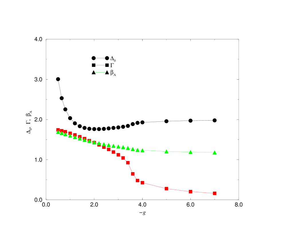
FIG. 6.: The $g$ dependence of thermodynamic variables $\Delta_{0}$, $\beta_{A}$ and $\Gamma$ for $g\eta=-0.01$. The calculations are done for the system size $N_{\phi}=16$, $N_{z}=8$.

FIG. 7.: The $g_{m}$ dependence of the discontinuity for $-\Delta_{0}$ and $E_{J}$ along the phase boundary between vortex liquid state and vortex solid state.

FIG. 8.: The top panel shows the distribution function for $S_{n,n}(G,0)$; the middle panel is a contour plot of the distribution function for $S_{n,n+4}(G,0)$ in the complex plane; the bottom panel is a contour plot of the distribution function for $\Delta_{n,n+4}(\vec{q}=0)/\Delta_{0}$ in the complex plane. All plots are at the melting transition point of a finite system with $N=6\times 6\times 8$, $g=-\sqrt{20.5}$, and $\eta=0.01$. $\vec{G}$ is a member of the first shell of reciprocal lattice vectors of the Abrikosov lattice.

FIG. 9.: The ratio of the largest eigenvalue of the density matrix to the sum of all eigenvalues, $Z$, as a function of $g$ at $\eta g=-0.045$. For this value of $g\eta$ a first order melting transition appears to occur at $g\sim-\sqrt{20.5}$. The size dependence of $Z$ at particular temperatures on the vortex solid and vortex liquid sides of the phase transition are shown in the right and left insets respectively.

REFERENCES

- [1] A.A. Abrikosov, Zh. Eksp. Teor. Fiz. 32, 1442 (1957).
- [2] D. R. Nelson, Phys. Rev. Lett. 60, 1415 (1988); P. L. Gammel, L. F. Schneemeyer, J. V. Wasczak, and D. J. Bishop, Phys. Rev. Lett. 61, 1666 (1988).
- [3] D. S. Fisher, M.P.A. Fisher and D. A. Huse, Phys. Rev. B. 43 130 (1991).
- [4] Jun Hu, A. H. MacDonald and B. D. McKay, Phys. Rev. B 49, 15263 (1994).
- [5] A.V. Nikulov, Supercond. Sci. Technol. 3, 377 (1990).
- [6] H. Safer, P. L. Gammel, D. A. Huse, and D. J. Bishop, Phys. Rev. Lett. 69, 824 (1992).
- [7] W. K. Kwok et al., Phys. Rev. Lett. 72, 1092 (1994).
- [8] E. Zeldov et. al., Nature 375 373 (1995).
- [9] R. Liang et al., Phys. Rev. lett. 76 835 (1996).
- [10] U. Welp et al., Phys. Rev. lett. 76 4809 (1996).
- [11] This paper is largely based on the Ph.D. thesis of one of us. Jun Hu, Ph.D. Thesis, Indiana University, 1994.
- [12] W. E. Lawrence and S. Doniach, in Proceedings of the Twelfth International Conference on Low Temperature Physics, Kyoto, Japan, 1971, edited by E. Kanda (Keigaku, Tokyo, 1971), p. 316.
- [13] Z. Tešanović and A. V. Andreev, Phys. Rev. B. 49, 4064 (1994); Ian D. Lawrie, Phys. Rev. B 50, 9456 (1994); R. Ikeda, J. Phys. Soc. Jpn. 64, 1683 (1995); Stephen W. Pierson, Oriol T. Valls, Zlatko Tešanovć, and Michael A. Lindemann, preprint (cond-mat/9702177) (1997).
- [14] Erik S. Sorensen and A.H. MacDonald, in preparation, to be submitted to Physical Review B.
- [15] Katerina Moloni, Mark Friesen, Shi Li, Victor Souw, P. Metcalf, Lifang Hou, and M. McElfresh, preprint (1996).
- [16] Similar calculations intended to model BSCCO and YBCO specifically have been reported by R. Šášik and D. Stroud, Phys. Rev. B. 48 9938 (1993) and Phys. Rev. Lett. 72 2462 (1994).
- [17] For a discussion of Cooper pair Landau levels and the mean-field-theory instability in terms of underlying electronic degrees of freedom see A.H. MacDonald, H. Akera, and M.R. Norman, Phys. Rev. B 45, 10147 (1992).
- [18] P.A. Lee and S.R. Shenoy, Phys. Rev. Lett. 28, 1025 (1972).
- [19] E. Brézin, D.R. Nelson, and A. Thiaville, Phys. Rev. B 31, 7124 (1985).
- [20] R.E. Hetzel, A. Sudbø, and D.A. Huse, Phys. Rev. Lett. 69, 518 (1992). See also A. Houghton, R.A. Pelcovits, and A. Sudbø, Phys. Rev. B 40, 6763 (1989); E.H. Brandt, Phys. Rev. Lett. 63, 1106 (1989); and D.R. Nelson and H.S. Seung, Phys. Rev. B 39, 9153 (1989).
- [21] Y.-H. Li and S. Teitel, Phys. Rev. B 47, 359 (1993), ibid 49, 4136 (1994), ibid 45 5718 (1992), Phys. Rev. Lett. 66 3301 (1991).
- [22] M.A. Moore, preprint cond-mat/9608105 (1996).
- [23] Y.-H. Li and S. Teitel, Phys. Rev. Lett. 66, 3301 (1991); Phys. Rev. B 47, 359 (1993); ibid 49, 4136 (1994); Tao Chen and S. Teitel, preprint (cond-mat/9610151) (1996); ibid, cond-mat/9702010 (1997).
- [24] A. K. Nguyen, A. Sudbø, and R.E. Hetzel, Phys. Rev. Lett. 77, 1592 (1996).
- [25] L.I. Glazman and A.E. Koshelev, Phys. Rev. B 43, 2835 (1991).
- [26] The approximation will often be accurate over a substantial portion of the fluctuation regime and describe the overall shape of magnetization and specific heat curves even when it is not accurate at the melting phase transition.
- [27] G. J. Ruggeri and D. J. Thouless, J. Phys. F 6, 2063 (1976).
- [28] Stephen W. Pierson, Oriol T. Valls, Zlatko Tešanovć, and Michael A. Lindemann, preprint (cond-mat/9702177) (1997).
- [29] Jun Hu and A. H. MacDonald, Phys. Rev. Lett. 71, 432 (1993).
- [30] G. Blatter et. al., Rev. Mod. Phys. 66 1125 (1994). E. H. Brandt, Reports on Progress in Phys. 58 1465 (1995).
- [31] For strongly type-II superconductors in fields which are a significant fraction of fluctuations in the internal magnetic field are negligible and will be ignored here. To leading order they can be accounted for perturbatively by replacing them by their thermodynamic averages. See D. J. Thouless, Phys. Rev. Lett. 34 946 (1975).
- [32] F.D.M. Haldane and E.H. Rezayi, Phys. Rev. B. 31 2529 (1985).
- [33] Z. Tešanović and Lei Xing, Phys. Rev. Lett. 67, 2729 (1991)
- [34] D.P. Arovas et. al, Phys. Rev. Lett. 60 619 (1988).
- [35] The line of argumentation is similar to that outlined in A.H. MacDonald and S.M. Girvin, Phys. Rev. B 38, 6295 (1988).
- [36] See for example, A.L. Fetter and P.C. Hohenberg, Chapter 14 in Superconductivity, Volume 2, edited by R. D. Parks (Dekker, New York, 1969).
- [37] M.V. Feigel’man, V.B. Geshkenbein, and A.I. Larkin, Physica C 167 177 (1990); E. Fray, D. R. Nelson, and D.S. Fisher, Phys. Rev. B 49, 9723 (1994).
- [38] J. Lee and J. M. Kosterlitz, Phys. Rev. Lett. 65, 137 (1990).
- [39] A. M. Ferrenberg and R. H. Swendsen, Phys. Rev. Lett. 61, 2635 (1988).
- [40] Y. Kato and N. Nagaosa, Phys. Rev. B. 48, 7383 (1993).
- [41] If so, we would not expect to see a double peak since for 2D systems these do not become obvious until the number of vortices approaches 100.
- [42] R. Šášik and D. Stroud used layers in their simulations of YBCO. Phys. Rev. Lett. 72, 2462 (1994).
- [43] W. R. White, A. Kapitulnik and M. R. Beasley, Phys. Rev. Lett. 66 2826 (1991).
- [44] P. Koorevaar, P.H. Kes, A. E. Koshelev and J. Aarts, Phys. Rev. Lett. 72 3250 (1994).
- [45] See for example, Kerson Huang Statistical Mechanics (Wiley, New York, 1963) p.37.
- [46] Jun Hu and A.H. MacDonald, Phys. Rev. B 52, 1286 (1995).
- [47] A similar analysis was independently developed by A. V. Nikulov, Phys. Rev. B. 52 10429 (1995).
- [48] The vortex lattice also expands on freezing in the London limit, although the physics responsible for this behavior is different. See Ref.[30] and D.R. Nelson in The Vortex State, edited by N. Bontemps et al. (Kluwer, Dordrecht, 1994).
- [49] We look at off-diagonal correlations at a separation of four layers since that is the largest layer separation in an layer system with periodic boundary conditions.
- [50] Z. Tešanović, Phys. Rev. B 51, 16204 (1995).
- [51] C.N. Yang, Rev. Mod. Phys. 34 694 (1962). For a recent perspective see see K. Huang in Bose-Einstein Condensation, edited by A. Griffin, D.W. Snoke, and S. Stringari (Cambridge University Press, Cambridge, 1995).
- [52] A. Houghton, R.A. Pelcovits, and A. Sudbø, Phys. Rev. B 42, 906 (1990); D.S. Fisher, M.P.A. Fisher, and D.A. Huse, Phys. Rev. B 43, 130 (1991); R. Ikeda, T. Ohmi, and T. Tsuneto, J. Phys. Soc. Jpn. 61, 254 (1992); M.A. Moore, Phys. Rev. B 45, 7336 (1992).
- [53] Z. Tešanović, Physica C 220, 303 (1994).
- [54] Jun Hu and A.H. MacDonald, in preparation.
- [55] Pinning is required for superconductivity perpendicular to the field, but its strength can vanish in the thermodynamic limit.
- [56] R. Šášik and D. Stroud, Phys. Rev. Lett. 75, 2582 (1995).
- [57] L.N. Bulaevskii, M. Ledvij, and V.G. Kogan, Phys. Rev. Lett. 68, 3733 (1992); Q. Li, M. Suenaga, G.D. Du, and N. Koshizuka, Phys. Rev. B 50, 6489 (1994); A. Wahl, A. Maignan, C. Martin, V. Hardy, J. Provost, and Ch. Simon, Phys. Rev. B 51, 9123 (1995).