[

Statistics of Earthquakes in Simple Models of Heterogeneous Faults

Abstract

Simple models for ruptures along a heterogeneous earthquake fault zone are studied, focussing on the interplay between the roles of disorder and dynamical effects. A class of models are found to operate naturally at a critical point whose properties yield power law scaling of earthquake statistics. Various dynamical effects can change the behavior to a distribution of small events combined with characteristic system size events. The studies employ various analytic methods as well as simulations.

]

The Gutenberg-Richter law [1] for the statistics of earthquakes — frequency inversely proportional to a power of the seismic moment — is well established over about 10 orders of magnitude. It is clearly a property of regional fault systems. The statistics of earthquakes on individual faults is much more controversial, indeed given the degree of geometrical complexity usually observed it is not even clear whether single faults are well defined. Nevertheless, statistics in various narrow fault zones in which slip is primarily along one direction — which we will henceforth refer to as “faults” — have been studied, and the behavior is found to vary substantially. In particular, Wesnousky[2] has found that faults with large total displacement which are relatively regular typically have a power law distribution only for small events — if at all — and events with a much larger characteristic size in which the whole fault slips, with few events in between. In contrast, less mature faults with more irregular geometries can have power law statistics over the whole range of observed magnitudes[2].

In this paper, we will show that simple models which include fault plane heterogeneities can exhibit both of these types of behavior and analyze the origin of the power law statistics and departures from it in these systems. In particular, we will argue that power law statistics can be understood quantitatively in terms of proximity to a specific non-equilibrium dynamical critical point. Like most critical points, the resulting exponents, although “universal”, will depend on certain properties in the system: the dimensionality, the range of interactions, randomness, and perhaps other aspects.

Most previous work on simple models has involved variants of the Burridge-Knopoff (or “sliderblock”) model in which the randomness is generated dynamically and inertia and friction laws play an essential role[3]. These systems appear to exhibit power law statistics over some range with a cutoff beyond some magnitude and with most of the slip occurring in larger, system size events. But the understanding of the origin of the power-law behavior is very limited. Our approach here will be to start with analytic understanding of a class of models and then add in various additional physical features by analytic scaling arguments in the framework of the renormalization group (RG), aided by numerical studies.

To investigate possible critical points, we first study infinite systems driven by a constant drive force $F$. The dynamical variables $u({\bf r},t)$ represent the discontinuity across the fault plane in the component of the displacement in the direction of slip. We consider general equations of motion of the form:

$$\eta\partial u({\bf r},t)/\partial t=F+\sigma({\bf r},t)-f_{R}[u({\bf r},t),{\bf r},\{u({\bf r},t^{\prime}<t)\}]$$ (1)

where

$$\sigma({\bf r},t)=\int\limits_{-\infty}^{t}dt^{\prime}\int d^{d}r^{\prime}J({\bf r}-{\bf r}^{\prime},t-t^{\prime})[u({\bf r}^{\prime},t^{\prime})-u({\bf r},t)]$$ (2)

is the stress and $f_{R}$ is a quenched random “pinning” force crudely representing inhomogeneities in the friction, asperities, stepovers etc., which in general can depend on the local past history (e.g. as in velocity dependent friction). The dynamics will be determined by this local history dependence, the stress transfer function $J({\bf r},t)$, and the coefficient $\eta$[4].

Substantial simplifications occur if $f_{R}$ is history independent and $J({\bf r},t)\geq 0$ for all $({\bf r},t)$; we will call these monotonic models. Related monotonic models have been studied extensively in various other contexts[5, 6]. Their crucial simplifying feature is that the steady state velocity $\overline{v}\equiv\langle\partial u/\partial t\rangle$ is a history independent function of $F$[7]. For $F$ less than a critical force $F_{c}$, $\overline{v}=0$, while just above $F_{c}$, $\overline{v}\sim(F-F_{c})^{\beta}$. Universal scaling behavior exists on large length scales near $F_{c}$. Quasi-static properties such as exponents and scaling functions depend on only a few quantities: the spatial dimension $d$; the range of the interactions if they are long-range, i.e. with the static stress transfer $J_{s}(r)\equiv\int dtJ(r,t)\sim 1/r^{d+\Gamma}$, with $\Gamma<2$; and the range of correlations in $f_{R}$, which we will generally assume are short-range in $u$ and ${\bf r}$. Long time dynamic properties such as $\beta$ depend in addition on the small $\omega$ dependence of $J({\bf q},\omega)$. If $F$ is adiabatically increased towards $F_{c}$, the system moves from one metastable configuration to another by a sequence of “quakes” of various sizes. The “quakes” can be characterized by their radius $R$, the $d$-dimensional area $A$ which slips (by more than some small cutoff), their moment $M\equiv\int d^{d}{\bf r}\Delta u({\bf r})$, a typical displacement $\Delta u\sim M/A$, and a duration $\tau$.

From RG expansions[5] around a dynamic mean field version of Eq. (1) and scaling arguments it is found that for large quakes $\Delta u\sim R^{\zeta}$, $A\sim R^{d_{f}}$ with $d_{f}\leq d$ a fractal dimension, $M\sim R^{{d_{f}}+\zeta}$ and $\tau\sim R^{z}$. The distribution of moments is

$$P(M)dM\sim dM/M^{1+B}\rho_{\infty}(M/\hat{M})$$ (3)

with $\rho_{\infty}$ a universal scaling function which decays exponentially for large argument. The cutoff $\hat{M}$ for large moments is characterized by a correlation length — the largest likely radius — $\xi\sim 1/(F_{c}-F)^{\nu}$ with $\hat{M}\sim\xi^{d_{f}+\zeta}$. In mean-field theory, $B=1/2$, the quakes are fractal and displacements are of order the range of correlations in $f_{R}(u)$, i.e. $\zeta=0$. The mean-field exponents are valid for $d>d_{c}(\tilde{\Gamma})=2\tilde{\Gamma}$ where $\tilde{\Gamma}\equiv{\it min}(\Gamma,2)$[6]. For a planar fault in an elastic half space, $d=2$ and $\Gamma=1$[8]; the physical system is thus at the upper critical dimension $d=d_{c}$[9].

As usual, at the upper critical dimension, there are logarithmic corrections to mean-field results. We find barely fractal quakes with $A\sim R^{2}/\ln R$ so that the fraction of the area slipped decreases only as $1/\ln r$ away from the “hypocenter”. The typical slip is $\Delta u\sim(\ln R)^{1/3}$ so that $M\sim R^{2}/(\ln R)^{2/3}$. The scaling form of $P(M)$ is the same as Eq. (3) with the mean-field $\rho_{\infty}$, although for $M<<\hat{M}$, $P(M)\sim(\ln M)^{1/3}/M^{3/2}$ so that $B$ will be virtually indistinguishable from $1/2$.

We now consider more realistic drive and finite-fault-size effects. Driving the fault by very slow motion far away from the fault is roughly equivalent to driving it with a weak spring, i.e. replacing $F$ in Eq. (1) by $F({\bf r},t)=K[vt-u({\bf r},t)]$. With $v\rightarrow 0$ the system must then operate with the spring stretched to make $F({\bf r},t)\lesssim F_{c}$ at least on average; it will actually operate just below $F_{c}$. Under a small increase, $\Delta F$, with constant force drive, $\langle\Delta u\rangle\approx n\Delta F\int MP(M)dM$ with $n$ the number of quakes per unit area per increase in $\Delta F$; $n(F)$ is non-singular at $F_{c}$[5]. The known scaling laws yield $\langle\Delta u\rangle\sim\Delta F\xi^{(2\tilde{\Gamma}+\zeta)(1-B)}\sim\Delta F\xi$ for our case. For consistency, we must have in steady state with the spring drive, $Kv\Delta t=\Delta F=K\Delta u$ so that the system will operate with a correlation length $\xi\sim 1/K^{1/\tilde{\Gamma}}$, i.e. $1/K$ for our case. For a fault section with linear dimensions of order $L$, drive either from uniformly moving fault boundaries or from a distance $\sim L$ perpendicularly away from the fault plane will be like $K\sim 1/L$ so that the power-law quake distribution will extend out to roughly the system size $\xi\sim L$. For smaller quakes, i.e. $R<<L$, the behavior will be the same as in the infinite system with constant $F$ drive, but the cutoff of the distribution of moments will be like Eq. (3) with a different cutoff function $\rho$ that depends on the shape of the fault, how it is driven, and the boundary conditions.

We have tested these conclusions numerically by studying a discrete space, time, and displacement version of a monotonic Eq. (1) with quasistatic stress transfer appropriate to an elastic half space[8]. The slip, $u$, is purely in the horizontal direction along the fault and $f_{R}[u({\bf r})]$ is a series of equal height spikes with spacings which are a random function of ${\bf r}$. When $\sigma({\bf r},t)>f_{R}[u({\bf r},t]$, $u({\bf r})$ jumps to the next spike. The boundary conditions on the bottom and sides are uniform slip — ($u=vt$) with infinitesimal $v$ — and stress free on the top. The statistics of the moments of the quakes are shown by the triangles in Fig. 1.

FIG. 1.: Histograms of moments for a simulation of a rectangular fault with 32x128 cells for the discrete monotonic quasistatic model. Triangles: without dynamical weakening ($\epsilon=0$). Diamonds: with dynamic weakening with $\epsilon=0.95$. ($\epsilon$ is defined in eq. (4).) The straight line indicates the predicted slope $B=1/2$.

Although the uncertainties are appreciable, relatively good agreement is found with the prediction $B=1/2$. A typical large quake is illustrated in Fig. 2 (a); it appears almost fractal as predicted and will tend to stay away from the bottom and sides. The ratios of the moments of quakes to their areas have been studied and found to grow only very slowly with the area, as predicted. This is in striking contrast to earthquakes in conventional crack models which are compact and have $\Delta u\sim R$ (i.e. $\zeta=1$), so that $M/A\sim\sqrt{A}$.

Because the system is at its critical dimension, the cutoff function $\rho$ of the moment distribution appropriate to the boundary conditions, as well as various aspects of the shapes and dynamics of quakes can be computed. For quasistatic stress transfer, $J({\bf r},t)\sim\delta(t)/r^{3}$, in the infinite system, the quake durations are found to be $\tau\sim R^{z}$ with $z<1$ for $d<d_{c}$, corresponding to an unphysical supersonic propagation of disturbances[6]. In the marginal dimension $d=d_{c}$, $z=1$ with logarithmic corrections. A more physical dynamics with sound-travel-time delay has slower growth of the quakes with $z=1$ in all dimensions. In either case the growth will be very irregular — including regions starting and stopping — in contrast to crack models and what is often assumed in seismological analyses of earthquakes.

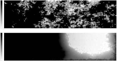
FIG. 2.: Distribution of horizontal slip, $u$, along a fault with 32x128 cells for a single large quake event. The lighter a cell the bigger its slip during the quake. Top (a) almost fractal quake with a total moment of 1750 (and 1691 cells failing) for the monotonic model without any dynamical effects ($\epsilon=0$). Bottom (b) “cracklike” quake with a total moment of 16922 (and 2095 cells failing) for the model with dynamic weakening ($\epsilon=0.95$). In both cases the system is driven by horizontally creeping fault boundaries (sides and bottom) while the top boundary is free.

A crucial feature of monotonic models is that the slip profile $\Delta u({\bf r})$ of a quake is independent of the dynamics[7]. But the most interesting dynamical issues concern the effects left out of the monotonic models that can make this feature breakdown. We first consider including some weakening effects of sections which have already slipped in a given quake. This is best studied in the discrete model. To crudely model a difference between static and dynamic friction we choose,

$$f_{R}=\tilde{f}_{R}[u({\bf r}),{\bf r}]\{1-\epsilon\Theta[u({\bf r},t)-u({\bf r},t-T)]\}$$ (4)

with $T$ a cutoff time much longer than the duration of the largest quakes, but much smaller than the interval between the quakes. This can crudely represent a difference between static and dynamic friction. For $\epsilon=0$ and non-negative $J$ the model is monotonic, while for $\epsilon>0$ it is non-monotonic. The effects of small weakening can be analyzed perturbatively.

With $\epsilon=0$, consider a quake of diameter $R_{1}$ ($<<L$ or $\xi$), with moment $M_{1}$ and area $A_{1}$: i.e. $A_{1}$ sites have slipped. If a small $\epsilon$ is turned on at the end of the quake, all slipped sites that are within $\epsilon$ of slipping will now slip again — this will be $N^{ex}_{2}\sim\epsilon A_{1}$ sites. The simplest justifiable guess is that each of these will cause an approximately independent secondary quake. The total moment of these secondary quakes will be dominated by the largest one, so the extra moment will be $M^{ex}_{2}\sim(\epsilon A_{1})^{1/B}$. If $M^{ex}_{2}<<M_{1}$ this process can continue but will not increase the total moment substantially. But if $M^{ex}_{2}\sim M_{1}$, the process can continue with a larger area $A_{2}$ and hence a larger $M^{ex}$, leading to runaway. The scaling laws yield $B=(d_{f}-\tilde{\Gamma}+\zeta)/(d_{f}+\zeta)$ and $A\sim M^{d_{f}/(d_{f}+\zeta)}$ with $\zeta<\tilde{\Gamma}$, so that for any $\epsilon$, for large enough $M_{1}$, $M_{1}\gtrsim M_{D}\sim\epsilon^{-(d_{f}+\zeta)/(\tilde{\Gamma}-\zeta)}$, $M^{ex}_{2}$ will be comparable to $M_{1}$ and the quake will become much larger. In the case of interest $M_{D}\sim\epsilon^{-2}$. In the force driven infinite system for $F\lesssim F_{c}$, quakes of size $\xi$ will runaway and become infinite if $\xi>\epsilon^{-1/(\tilde{\Gamma}-\zeta)}$. Since $\xi\sim(F-F_{c})^{-\nu}$ and $1/\nu=\tilde{\Gamma}-\zeta$, this will occur for $F_{c}-F<C_{w}\epsilon$ with some constant $C_{w}$. This result is very intuitive and justifies a posteriori the assumptions leading to it: Since on slipping, the random pinning forces, $f_{R}$ in a region are reduced by order $\epsilon$, the effective critical force $F_{c}$ for continuous slip will have been reduced by order $\epsilon$; thus if $F>F_{c}(\epsilon)=F_{c}-C_{w}\epsilon$, the mean velocity $\overline{v}$ will be nonzero.

A similar but more subtle effect can be caused by stress pulses that result from non-positive $J({\bf r},t)$; these arise naturally when one includes elastodynamic effects. We consider

$$J({\bf r},t)\sim\delta(t-r/c)/r^{d+\Gamma}+\alpha\delta^{\prime}(t-r/c)/cr^{d+\gamma}$$ (5)

with $c$ the sound speed. The scalar approximation to elasticity in a half space corresponds to $d=2$, $\Gamma=1$, $\gamma=0$, and $\alpha=1$. If a region slips forward, the stress at another point first has a short pulse at the sound arrival time from the second term in Eq. (5), then settles down to its smaller static value, i.e. it is non-monotonic. The magnitude of these stress pulses and their duration is set by various aspects of the models, for example larger $\eta$ in Eq. (1) implies weaker stress pulses as the local motion will be slower. By considering which of the sites in a long quake with $\alpha=0$ can be caused to slip further by such stress pulses — here the dynamics matters — we find that runaway will occur for $M\geq M_{D}\sim\alpha^{-4}$ for the physical case. We have checked this in $d=1$ with $\Gamma=1$ and $\gamma=0$ finding the predicted reduced critical force $F_{c}(\alpha)\sim F_{c}-C_{p}\alpha^{2}$ as shown in Fig. 3. These 1-d simulations also reveal a hysteretic $\overline{v}(F)$ curve in finite systems. This should also occur with the velocity weakening model.

We can now understand what should happen with either weakening or stress pulses in finite systems driven with a weak spring or with slowly moving boundaries. As the system is loaded, quakes of increasing size can occur. If the system is small enough that it cannot sustain quakes with $M>M_{D}(\epsilon,\alpha)$ then the behavior will not be much different from the monotonic case with $\epsilon=\alpha=0$. This will occur if $L<R_{D}(\epsilon,\alpha)\sim M_{D}^{1/2}\sim{\it max}(C_{\alpha}/\alpha^{2},C_{\epsilon}/\epsilon)$ with appropriate coefficients $C_{\alpha}$, $C_{\epsilon}$, which will depend on the amount of randomness in the fault. But if $L>R_{D}$, quakes of size of order $R_{D}$ will runaway and most of the system will slip, stopping only when the load has decreased enough to make the loading forces less than the lower end of the hysteresis loop in ${\overline{v}}(F)$ (as in Fig. 3).

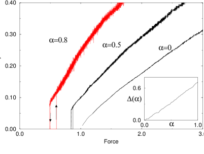
FIG. 3.: Mean velocity versus force for one dimensional system with a non-monotonic kernel $J(x,t)=\delta(t-x)/x^{2}+\alpha\delta{{}^{\prime}}(t-x)/x$ for $\alpha=0.8,0.5,0$. A spring or boundary loaded system will traverse the hysteresis loops in the direction indicated. Inset: the threshold force, $F_{c}^{\uparrow}(\alpha)$, on increasing the load; $\Delta_{\alpha}=[1-F_{c}^{\uparrow}(\alpha)/F_{c}^{\uparrow}(\alpha=0)]^{1/2}$ is plotted vs. $\alpha$.

Because of the tendency of regions that have already slipped to slip further, and the consequent buildup of larger stresses near the boundaries of the slipped regions, large events in systems with dynamic weakening will be much more cracklike than in monotonic models, probably with $\Delta u\sim L$. Statistics of quakes with weakening, $\epsilon$, reasonably large, but no stress pulses ($\alpha=0$) are shown in Fig. 1 and in [8]; note the absence of quakes with intermediate moments. A typical large event in this case is shown in Fig. 2 (b); it appears to be crack-like.

In this paper we have shown that simple models of heterogeneous faults — with the dimensionality and long-range elastic interactions properly included — can give rise to either power-law statistics of earthquake moments or a distribution of small events combined with characteristic system size events. Which behavior — or intermediate behavior — obtains is found to depend on a number of physical properties such as frictional weakening and dynamic stress transfer, analogs of which should definitely exist in real systems. In the power-law-regime the conventionally defined Gutenberg-Richter exponent $b\equiv 3B/2$ is is found to be $b=3/4$. This is intriguingly close to values observed by Wesnousky[2], but it is not clear if any significance should be attached to this.

More significant is the framework that we have built, which enables certain results (and many more not presented here) to be obtained analytically and others to be understood by scaling arguments. It is hoped that other physical phenomena such as geometrical disorder, side branching, and multiple cracks might start to be addressed in this framework. We note one extra effect which can be readily analyzed: long range correlations in the randomness (perhaps caused by prior history of the fault). Varying the power-law of the decay of correlations of $f_{R}$ increases $B$ continually from $1/2$ to $2/3$ and $\zeta$ concomitantly from 0 to 1 with the quakes becoming more compact and crack-like as the randomness correlations become longer range.

We would like to thank Jim Rice, Deniz Ertas, Chris Myers, and Jim Sethna for many useful conversations. This work is supported in part by the Harvard Society of Fellows and by NSF via DMR 9106237, 9630064 and Harvard’s MRSEC.

REFERENCES

- [1] B. Gutenberg, and C.F. Richter, Ann. Geophys. 9, 1 (1956).
- [2] S.G. Wesnousky Bull. Seismol. Soc. Am. 84, 1940, 1994.
- [3] J.M. Carlson, J.S. Langer, B.E. Shaw, Rev. Mod. Phys. 66, 658, 1994, and references therein; C.R. Myers, B.E. Shaw, J.S. Langer, Phys. Rev. Lett. 77, 972 (1996); J.B. Rundle, W. Klein, S. Gross Phys. Rev. Lett. 76 4285 (1996).
- [4] Linear velocity-strengthening friction can be absorbed into .
- [5] O. Narayan and D. S. Fisher, Phys. Rev. Lett. 68, 3615 (1992); Phys. Rev. B 46, 11520 (1992); Phys. Rev. B 48, 7030 (1993); Phys. Rev. B 49, 9469 (1994); O. Narayan and A.A. Middleton Phys. Rev. B 49, 244 (1994); T. Nattermann, S. Stepanow, L.H. Tang and H.Leschhorn J. Phys. II France 2, 1483 (1992); J.P. Sethna et al. Phys. Rev. Lett. 70, 3347 (1993); K. Dahmen and J. P. Sethna Phys. Rev. B53, 14872 (1996), and references therein; D. Cule, T. Hwa Phys. Rev. Lett. 77, 278 (1996).
- [6] D. Ertaş and M. Kardar, Phys. Rev. E 49, R2532 (1994); Phys. Rev. Lett. 73, 1703 (1994).
- [7] A.A. Middleton, Phys. Rev. Lett. 68, 670, 1992.
- [8] Y. Ben-Zion and J.R. Rice, J. Geophys. Res. 98, 14109, 1993; Y. Ben-Zion and J.R. Rice, J. Geophys. Res. 100, 12959, 1995; Y. Ben-Zion J. Geophys. Res. 101, 5677, 1996.
- [9] In contrast, for very large quakes that rupture through the whole depth of the crust, the fault becomes essentially one dimensional with , although the different boundary conditions etc. will make our analysis not applicable.