Criticality in the Integer Quantum Hall Effect

Alex Hansen, E. H. Hauge, Joakim Hove and Frank A. Maaø

Institutt for fysikk, Norges teknisk-naturvitenskapelige universitet, NTNU

N–7034 Trondheim, Norway

We review some elementary aspects of the critical properties of the series of metal-insulator transitions that constitute the integer quantum Hall effect. Numerical work has proven essential in charting out this phenomenon. Without being complete, we review network models that seem to capture the essentials of this critical phenomenon.

1. Introduction

The existence of localized states in semiconductors has been known since the seminal work of Anderson [1,2]. He used a deceptively simple-looking tight-binding model and showed that when the disorder of the binding energy on the scale set by the interaction energy exceeds a given limit (which is zero in one dimension), the wave functions are localized in space. I.e. the eigenstates fall off exponentially while still forming a continuous energy spectrum. The physics behind this mechanism is destructive interference. Another mechanism that leads to localization is that of percolation, for the first time described by Flory [3], and later used by Skal and Shklovskii [4] to describe hopping resistivity of lightly doped semiconductors. Percolation theory has, however, grown far beyond semiconductor physics, and even beyond physics. For a modern review, see, e.g., Sahimi [5]. The review by Thouless [6] discusses percolation and Anderson localization in a unified manner.

In this paper, we shall discuss localization in the integer quantum Hall effect. The classical Hall effect is standard textbook material, see e.g., Ashcroft and Mermin [7]. A conductor in the shape of a thin rectangular plate, i.e. a Hall bar, is placed in the strong perpendicular magnetic field $\vec{B}$ as shown in Fig. 1. A current $I_{x}$ flows through the bar, giving rise to a longitudinal voltage drop $V_{x}$ and a transversal voltage drop $V_{y}$, which is also called the Hall voltage. It is the appearance of this transversal voltage that constitutes the classical Hall effect. The ratios

$$\rho_{xx}={{V_{x}}\over{I_{x}}}\;,$$

and

$$\rho_{yx}={{V_{y}}\over{I_{x}}}$$

define the longitudinal resistance and Hall resistance respectively. Simple arguments based on the Drude model of conductance predict the longitudinal resistance to be independent of the magnetic field $\vec{B}$, and the Hall resistance to be linear in $B=|\vec{B}|$. This is also found experimentally.

Figure 1: Schematic diagram of the Hall system

Using a Si MOSFET inversion layer — which forces the charge carriers to move in a two-dimensional plane — placed in a 19 Tesla magnetic field and at a temperature of 1.5 K, von Klitzing et al. [8] observed a completely different behavior of the two resistances: The longitudinal resistance showed a series of pronounced peaks while being zero between them. The Hall resistance did not grow linearly with $B$, but developed a series increasingly pronounced steps. The reader should take a look at Paalanen et al. [9] to see these plots, which here are based on a GaAs heterostructure (as they did not appear explicitly in the original von Klitzing et al. paper). This is the integer quantum Hall effect. We have listed in Table 1 the typical values of some relevant physical quantities in the GaAs heterostructure.

The behavior of the longitudinal resistance clearly indicates that the charge carriers of the quantum Hall system repeatedly localizes and delocalizes with increasing magnetic field. What kind of localization goes on, and why the repeated localization-delocalization-localization transitions? These questions lie at the heart of the integer quantum Hall effect.

Several very good texts on the integer (and fractional) quantum Hall effect have already appeared, see e.g. Ref. [10–13]. Our aim with this paper is to convey an elementary understanding of the phenomenon, rather than a full-scale review of the entire literature. We therefore urge the readers to consult these more complete works.

We should perhaps apologize that the parts of this review that deal with the numerical studies of the integer quantum Hall effect is short compared to those dealing with describing the physics of the system. However, we believe this to be justified. The numerical models are simple, but the results that they lead to are profound. In order for the reader to appreciate the numerical models fully, we have chosen to emphasize the physics of the effect. We write this review for an audience in mind with a background in statistical

    $m=0.067m_{e}$ Effective mass $n=4\cdot 10^{15}{\rm m}^{-2}=(16{\rm nm})^{-2}$ Electron sheet density $E_{F}=14$meV Fermi energy $\lambda_{F}=40$nm Fermi wavelength $\Lambda=10^{2}$ – $10^{4}$nm Elastic mean free path $\Lambda_{\phi}>\Lambda$ Phase coherence length $l=\sqrt{\hbar/eB}=26(B/{\rm T})^{-1/2}$nm Magnetic length    

Table 1: Some relevant physical quantities in the GaAs heterostructure

physics. We have therefore attempted to be quite thorough and explicit in setting up the physical framework. No prior knowledge to the problem of two-dimensional quantum transport is assumed, and only elementary quantum mechanics is used. The essence of what will follow is this: The integer quantum Hall effect is closely related to the Landau levels of the electrons, formed when the system is placed in a strong perpendicular magnetic field. The energy of the electrons is quantized in way similar to the harmonic oscillator, see Eqs. (13) and (15). Whenever the magnetic field is reduced and one of these Landau levels in the bulk sinks through the Fermi level of the electrons, an additional contribution to the electrical conductance is made possible by filling this new Landau level with electrons from the attached reservoirs. This leads to the quantized current of Eq. (68) and to the subsequent “hydrodynamical” scenario thereafter in which disorder plays a crucial rôle.

The organization of the review is as follows: We discuss in the next section the behavior of a two-dimensional free electron gas in a strong perpendicular magnetic field. The integer quantum Hall effect enters in a very subtle way in this simple model. When we introduce interactions between the underlying lattice and the electrons, the integer quantum Hall effect becomes much more robust — and easy to understand. We discuss this in Sec. 3. As will be evident from this section, percolation plays an important rôle. In Sec. 4, we discuss the critical behavior of the integer quantum Hall system, which is caused by localization-delocalization transitions when the the externally applied magnetic field is changed. We furthermore discuss a famous semi-classical argument that seemingly identifies the nature and thus the universality class of these transitions. Unfortunately, there are problems with this argument, as we point out. In Sec. 5, we discuss a class of numerical network models that seems to capture the critical behavior of the quantum Hall system very well. Section 6. contains our conclusions.

2. The Free Electron Gas in a Closed System

The Hamiltonian of an electron moving in the $(x,y)$ plane and in a perpendicular, constant magnetic field $\vec{B}=B\vec{e}_{z}$ is

$$H_{0}={1\over{2m}}\left(\vec{p}+e\vec{A}\right)^{2}\;,$$

where $\vec{B}=\vec{\nabla}\times A$, $e$ is the elementary charge and $m$ the effective mass. We shall temporarily not specify any particular gauge. The standard commutation relations apply:

$$[x,p_{x}]=[y,p_{y}]=i\hbar\;,$$

and

$$[x,y]=[p_{x},p_{y}]=[x,p_{y}]=[y,p_{x}]=0\;.$$

Following Kubo et al. [14], we perform a canonical transformation from the original coordinates $(x,y)$ and $(p_{x},p_{y})$ to the relative coordinates $(\xi,\eta)$ and guiding center coordinates $(X,Y)$:

$$\xi={1\over{eB}}\left(p_{y}+eA_{y}\right)\;,$$

$$\eta=-{1\over{eB}}\left(p_{x}+eA_{x}\right)\;,$$

$$X=x-\xi\;,$$

and

$$Y=y-\eta\;.$$

The commutation relations (4) and (5) lead to

$$[X,Y]=-[\xi,\eta]=i\left({{\hbar}\over{eB}}\right)=il^{2}\;,$$

and

$$[\xi,X]=[\eta,Y]=[\xi,Y]=[\eta,X]=0\;.$$

In Eq. (10), we have used the magnetic length

$$l^{2}={\hbar\over{eB}}\;,$$

which corresponds to the cyclotron radius for the lowest quantum state. The accompanying classical cyclotron frequency is

$$\omega={{eB}\over{m}}\;.$$

The relative coordinates $\xi$ and $\eta$ describe the position of the electron relative to the center of the circle on which the electron is moving. The position of this center, the guiding center, is given by $X$ and $Y$. The Hamiltonian is in these coordinates

$$H_{0}={m\over{2}}\omega^{2}\left(\xi^{2}+\eta^{2}\right)\;,$$

which we recognize as the harmonic oscillator Hamiltonian by appealing to the commutation relation (10). The energy spectrum is therefore

$$E_{n}=\hbar\omega\left(n+{1\over 2}\right)\;.$$

These are the Landau levels.

In order to construct the wave functions, we must specify a gauge. We choose the Landau gauge where $\vec{A}^{x}=(-By,0)$. The Schrödinger equation then becomes

$$-{{\hbar^{2}}\over{2m}}\left[{{\partial^{2}}\over{\partial y^{2}}}+\left({{\partial}\over{\partial x}}-{{ieB}\over{\hbar}}y\right)^{2}\right]\psi_{n}^{x}=E_{n}\psi_{n}^{x}\;,$$

where the superscript $x$ refers to the choice of gauge that we have made. We now set

$$\psi_{n,Y}^{x}(x,y)={{e^{ikx}}\over{\sqrt{L}}}\tilde{\chi}_{n}(y)\;,$$

so that Eq. (16) becomes

$$\left[-{{\hbar^{2}}\over{2m}}{{d^{2}}\over{dy^{2}}}+{{m}\over 2}\omega^{2}\left(y-kl^{2}\right)^{2}\right]\tilde{\chi}_{n}(y)=E_{n}\tilde{\chi}(y)\;.$$

Thus, the energy eigenfunctions $\psi_{n,Y}^{x}$ consist of plane waves in the positive $x$ direction and harmonic oscillator wave functions $\tilde{\chi}_{n}(y)=\chi_{n}(y-kl^{2})$ in the $y$ direction centered around $Y=kl^{2}$. The energy levels are independent of $k$. The energy eigenfunctions are therefore

$$\psi^{x}_{n,Y}(x,y)={{e^{iYx/l^{2}}}\over{\sqrt{L}}}\chi_{n}(y-Y)\;.$$

These eigenfunctions form a complete set, and any wave function may be written

$$\psi^{x}(x,y)=\sum_{n}\int dY{{e^{iYx/l^{2}}}\over{\sqrt{L}}}\chi_{n}(y-Y)C_{n}(Y)\;.$$

A change of gauge $\vec{A}\to\vec{A}-\vec{\nabla}\alpha$ leads to a change in phase of the wave function, $\psi\to\exp(ie\alpha/\hbar)\psi$. For example, we may go from Landau gauge $\vec{A}^{x}=(-By,0)$ to the symmetric gauge $\vec{A}^{s}=(-By/2,Bx/2)$. Integrating the difference between these, $\vec{\nabla}\alpha=$$(-By/2,-Bx/2)$, gives $\alpha=-Bxy/2$. An arbitrary wave function in this gauge may therefore be written

$$\psi^{s}(x,y)=\sum_{n}\int dY{{e^{-i(xy-2Yx)/2l^{2}}}\over{\sqrt{L}}}\chi_{n}(y-Y)C_{n}(Y)\;.$$

Let us now count the number of states per Landau level and per area in the system. Assuming periodic boundary conditions in the $x$ direction, the wave function (17) must be periodic in the length $L$ of the system, $\psi_{n,Y}^{x}(x+L,y)=\psi_{n,Y}^{x}(x,y)$. This quantizes the possible values of $Y$,

$$Y={{2\pi l^{2}}\over L}j\;,$$

where $j=0,\pm 1,\pm 2,\cdots$. The system has width $W$ in the $y$ direction. Thus, $0\leq Y\leq W$ — remember that $Y$ determines the center of the harmonic oscillator wave functions in the $y$ direction. Combination of this restriction with Eq. (22), leads to $j$ being confined to the integers on the interval $0\leq j\leq LW/2\pi l^{2}=j_{\max}$. Thus, the number of states per Landau level per area is

$$n_{B}={{j_{\max}}\over{LW}}={1\over{2\pi l^{2}}}\;.$$

We now turn on an electric field $\cal E$ in the $y$ direction. The Hamiltonian (14) then becomes

$$H={m\over 2}\omega^{2}\left(\xi^{2}+\eta^{2}\right)+e{\cal E}_{y}\left(Y+\eta\right)\;,$$

where we have used Eq. (9), $y=Y+\eta$. We may rewrite this Hamiltonian as

$$H={m\over 2}\omega^{2}\left(\xi^{2}+\left(\eta+{{e{\cal E}_{y}}\over{m\omega^{2}}}\right)^{2}\right)-{{e^{2}{\cal E}_{y}^{2}}\over{2m\omega^{2}}}+e{\cal E}_{y}Y\;.$$

From this it is possible to write down the eigenfunctions and corresponding energy levels directly by inspection:

$$\psi^{x}_{n,Y}(x,y)={{e^{iYx/l^{2}}}\over{\sqrt{L}}}\chi_{n}\left(y-Y+{{e{\cal E}_{y}}\over{m\omega^{2}}}\right)\;,$$

and

$$E_{n,Y}=\hbar\omega\left(n+{1\over 2}\right)+e{\cal E}_{y}\left(Y-{{e{\cal E}_{y}}\over{m\omega^{2}}}\right)+{m\over 2}\left({{{\cal E}_{y}}\over{B}}\right)^{2}\;,$$

where the second term represents potential energy in the electric field and the third term the kinetic energy associated with guiding-center drift.

Let us now calculate the current densities in the system. Essential ingredients of such a calculation are the expectation values of the velocity in the $x$ and $y$ directions,

$$v_{x}(n,Y)=\int dx\ dy\ {\psi^{x}_{n,Y}}^{*}(x,y)\dot{x}\psi^{x}_{n,Y}(x,y)\;,$$

and

$$v_{y}(n,Y)=\int dx\ dy\ {\psi^{x}_{n,Y}}^{*}(x,y)\dot{y}\psi^{x}_{n,Y}(x,y)\;.$$

We split $\dot{x}$ and $\dot{y}$ into $\dot{x}=\dot{\xi}+\dot{X}$ and $\dot{y}=\dot{\eta}+\dot{Y}$. The Heisenberg equations of motion give

$${{d\xi}\over{dt}}={{i}\over{\hbar}}[H,\xi]=-\omega\left(\eta+{{e{\cal E}_{y}}\over{m\omega^{2}}}\right)\;,$$

$${{d\eta\ }\over{dt}}={{i}\over{\hbar}}[H,\eta]=+\omega\xi\;,$$

$${{dX}\over{dt}}={{i}\over{\hbar}}[H,X]={{el^{2}}\over{\hbar}}\ {\cal E}_{y}={{{\cal E}_{y}}\over B}\;,$$

and

$${{dY}\over{dt}}={{i}\over{\hbar}}[H,Y]=0\;.$$

We have here used the commutation relations Eqs. (10) and (11), and the Hamiltonian, Eq. (24). Combining these results with equations (28) and (29) give

$$v_{x}(n,Y)={{{\cal E}_{y}}\over{B}}\;,$$

and

$$v_{y}(n,Y)=0\;.$$

In Eq. (34) we have used that

$$\int_{-\infty}^{\infty}d\eta\ |\chi_{n}(\eta+e{\cal E}_{y}/m\omega^{2})|^{2}(\eta+e{\cal E}_{y}/m\omega^{2})=\int_{-\infty}^{\infty}d\eta\ |\chi_{n}(\eta)|^{2}\eta=0\,.$$

In equation (35), we have used that

$$\int_{-\infty}^{\infty}d\eta\ \chi_{n}(\eta+e{\cal E}_{y}/m\omega^{2})^{*}\xi\chi_{n}(\eta+e{\cal E}_{y}/m\omega^{2}) =$$

$$\int_{-\infty}^{\infty}d\eta\ \chi_{n}(\eta+e{\cal E}_{y}/m\omega^{2})^{*}(-il^{2}){{d}\over{d\eta\ }}\chi_{n}(\eta+e{\cal E}_{y}/m\omega^{2}) = 0\;.$$ (37)

With $n_{e}$ electrons per area, Eqs. (34) and (35) give rise to a current density in the $x$ direction equal to

$$j_{x}=-\sum_{n,Y}ev_{x}(n,Y)=-2\pi l^{2}{n_{e}}{{e^{2}}\over{h}}\ {\cal E}_{y}=-{{n_{e}}\over{n_{B}}}\ {{e^{2}}\over{h}}\ {\cal E}_{y}=-{{e^{2}\nu}\over{h}}\ {\cal E}_{y}\;.$$

The sum runs over all electrons and we ignore spin. In the $y$ direction the current density is

$$j_{y}=-\sum_{n,Y}ev_{y}(n,Y)=0\;.$$

We have in Eq. (38) defined the filling factor

$$\nu={{n_{e}}\over{n_{B}}}\;.$$

$n_{B}$ is defined in Eq. (23).

From Eqs. (38) and (39), we read off the elements of the conductivity

$$\sigma_{xx}=\sigma_{yy}=0\;,$$

and

$$\sigma_{yx}=-\sigma_{xy}={{e^{2}}\over{h}}\ \nu\;.$$

From this the resistance tensor follows by inversion, or directly by reference to Eqs. (1) or (2) as

$$\rho_{xx}=\rho_{yy}=0\;.$$

and

$$\rho_{xy}=-\rho_{yx}={{h}\over{e^{2}\nu}}\;.$$

The resistances (43) and (44) capture one aspect of what is measured in the integer quantum Hall effect: zero longitudinal resistance. However, the steps, which have their centers at integer values of the filling factor $\nu$ and the onset of longitudinal conductance when the system moves from one step to the next, are not found in this system. The reason that the steps are not visible, is that the system is closed. In Sec.  3.2, we will consider an open system, where steps do appear. The reason why steps only appear in open systems will be clear at that point. Before we turn to this discussion, we add interactions between the electrons and the underlying system, as they play a crucial rôle in what happens between the steps — which is the subject of this review.

3. Interactions between Electrons and Lattice: The Disordered Potential

We now add an arbitrary potential $V(x,y)$ to the Hamiltonian (3). The Schrödinger equation we have to solve is then

$$H\psi(x,y)=H_{0}\psi(x,y)+V(x,y)\psi(x,y)=E\psi(x,y)\;.$$

We expand the wave function as in Eq. (20) In this basis, we have that

$$H_{0}\psi^{x}(x,y)=\sum_{n^{\prime}}\hbar\omega\left(n^{\prime}+{1\over 2}\right)\int dY^{\prime}\ e^{iY^{\prime}x/l^{2}}\chi_{n^{\prime}}(y-Y^{\prime})C_{n^{\prime}}(Y^{\prime})/{\sqrt{L}}\;.$$

By multiplying Eq. (45) by $e^{-iYx/l^{2}}\chi^{*}_{n}(y-Y)/\sqrt{L}$ and integrating over $(x,y)$, the Schrödinger equation is transformed into

$$\int dx\ dy\ V(x,y)\sum_{n^{\prime}}\int dY^{\prime}\ e^{i(Y^{\prime}-Y)x/l^{2}}\chi^{*}_{n}(y-Y)\chi_{n^{\prime}}(y-Y^{\prime})C_{n^{\prime}}(Y^{\prime})/2\pi l^{2}$$

$$=(E-E_{n})C_{n}(Y)\;.$$ (47)

This expression is similar, but not identical, to the one given by Tsukada [15], which is the standard reference, but contains a small error.

Let us now make some changes of variables in Eq. (47). By defining $\Delta_{Y}=Y^{\prime}-Y$ and using that $x=X+\xi$ and $y=Y+\eta$, we can write Eq. (47) as

$$\int d\xi d\eta\ V(X+\xi,Y+\eta)\int d\Delta_{Y}{{e^{i\Delta_{Y}(X+\xi)/l^{2}}}\over{2\pi l^{2}}}$$

$$\sum_{n^{\prime}}\chi^{*}_{n}(\eta)\chi_{n^{\prime}}(\eta-\Delta_{Y})C_{n^{\prime}}(Y+\Delta_{Y}) = (E-E_{n})C_{n}(Y)\;.$$ (48)

So far, we have made no approximations. However, from now on we shall assume that $V(x,y)$ is slowly varying on the scale of the magnetic length $l$. Since the functions $\chi_{n}(x)$ are localized over distances of the order of $l$ — they are harmonic oscillator eigenfunctions — we may substitute $V(x,y)$ by $V(X,Y)$ in Eq. (48) as the lowest order term in an expansion in $l$. With this substitution, Eq. (48) simplifies dramatically by first integrating over $\xi$ and then using the orthonormality of the basis functions $\chi_{n}$,

$$V(X,Y)C_{n}(Y)=(E-E_{n})C_{n}(Y)\;.$$

The corresponding energy eigenfunctions are

$$\psi^{x}_{n}(x,y)=\int dY{{e^{iYx/l^{2}}}\over{\sqrt{L}}}\chi_{n}(y-Y)C_{n}(Y)\;.$$

What is the physical contents of Eq. (49)? In the classical limit, where $X$ and $Y$ are treated as c-numbers, it predicts a motion that follows the equipotential curves of $V(x,y)=E-E_{n}$. The classical electrons move in a strong magnetic field such that they neither gain nor loose energy. In order to expand on this, we write down the Heisenberg equations of motion for $X$ and $Y$:

$${{dX}\over{dt}}={{i}\over{\hbar}}[H,X]=+{1\over{eB}}\ {{\partial V}\over{\partial y}}\;,$$

and

$${{dY}\over{dt}}={i\over{\hbar}}[H,Y]=-{1\over{eB}}\ {{\partial V}\over{\partial x}}\;,$$

where $H=H_{0}+V$, where $H_{0}$ is given in Eq. (3), and we have used the commutation relations (10) and (11). There are no approximations in Eqs. (51) and (52). Introducing the same level of approximation as was done to arrive at Eq. (49), i.e., assuming that $V$ is slowly varying on the scale of the magnetic length $l$, Eqs. (51) and (52) become

$${{dX}\over{dt}}=+{1\over{eB}}\ {{\partial V}\over{\partial Y}}\;,$$

and

$${{dY}\over{dt}}=-{1\over{eB}}\ {{\partial V}\over{\partial X}}\;.$$

These equations are also valid in the classical limit. Let us now multiply the velocity vector of the guiding centers $(\dot{X},\dot{Y})$ with the gradient of the potential, $\vec{\nabla}V=(\partial V/\partial X,\partial V/\partial Y)$. We then get $\dot{\vec{U}}\cdot\vec{\nabla}V=0$ by use of Eqs. (53) and (54). Here $\vec{U}=(X,Y)$. Thus, the motion of the guiding center is always orthogonal to the local gradient of the interaction potential, and as a consequence, the guiding centers follow the equipotential curves of $V$.

3.1 Motion Near a Saddle Point: Tunneling

There will be quantum mechanical tunneling if two distinct equipotential lines come close at some point in space, as shown in Fig. 2. This may be somewhat surprising in that the tunneling has to appear in the direction orthogonal to the paths. We may understand this qualitatively through the following semi-classical picture: The paths drawn as in Fig. 2 are those of the guiding centers, which the electron itself is rotating about. Thus, the momentum vector of the electron points in “all” directions, even orthogonal to the path that the guiding center is following — making tunneling possible in the seemingly most unlikely direction.

Figure 2: The potential $V$ has a saddle point in region $A$. Even if the two paths marked in bold, which follow the equipotential curves of $V$, are antiparallel where they are at the closest, there is tunneling between them.

Let us analyse this transverse tunneling more closely. Following Fertig [19] and Mil’nikov and Sokolov [20], we concentrate on the region near a saddle point of $V$. We choose a coordinate system so that the saddle point is placed at the origin. Furthermore, we orient the coordinate system so that close to the origin, we have that

$$V(X,Y)=V_{0}-\alpha X^{2}+\beta Y^{2}\;,$$

where $\alpha>0$ and $\beta>0$. Thus, $V$ has a local maximum at the origin when moving along the $X$ axis, and a local minimum at the origin when moving along the $Y$ axis. Two situations may then occur: (1) $E-E_{n}<V(0,0)=V_{0}$, where $E$ is found by solving the Schrödinger equation (49). The corresponding semi-classical paths are shown in Fig. 3a. Likewise, the situation when $E-E_{n}>V_{0}$ is shown in Fig. 3b. Suppose that the situation is that of Fig. 3a. Then, it is convenient to use the representation $Y=il^{2}d/dX$, thus satisfying the commutator $[X,Y]=il^{2}$, Eq.  (10). Equation (49) then becomes

$$\left(-\beta l^{4}{{d^{2}}\over{dX^{2}}}-\alpha X^{2}\right)C_{n}(X)=\left(E-E_{n}-V_{0}\right)C_{n}(X)\;.$$

If, on the other hand, the situation is the one described in Fig. 3b, we switch to the representation $X=-il^{2}d/dY$, which also satisfies the commutation rule $[X,Y]=il^{2}$. Equation (49) then takes the form, after an overall change of sign,

$$\left(-\alpha l^{4}{{d^{2}}\over{dY^{2}}}-\beta Y^{2}\right)C_{n}(Y)=\left(V_{0}+E_{n}-E\right)C_{n}(Y)\;.$$

Figure 3: The potential $V$ has a saddle point at the origin. In (a) we show two semi-classical paths corresponding to $E<E_{n}+V_{0}$, and in (b) we show the paths corresponding to $E>E_{n}+V_{0}$.

Thus, we are faced with solving the one-dimensional scattering problems posed by the Schrödinger Eqs. (56) and (57) in order to study tunneling. This is difficult since $|V|\to\infty$ when $|X,Y|\to\infty$. However, we can get around this difficulty by substituting $V_{0}-\alpha X^{2}\to V_{0}/\cosh^{2}(\sqrt{\alpha/V_{0}}X)$ in Eq. (56) or $-V_{0}+\beta Y^{2}\to V_{0}/\cosh^{2}(\sqrt{\beta/V_{0}}Y)$ in Eq. (57), see Hansen [21]. This substitution leads to the correct quadratic behavior near the origin, and plane-wave solutions far away from the origin. The exact solution of the resulting one-dimensional scattering problem may be found, e.g., in ter Haar [22] or Landau and Lifshitz [23]. Both Eqs. (56) and (57) lead to a transmission coefficient

$$T={{P}\over{1+P}}\;,$$

where

$$P=e^{-2\pi/l^{2}\sqrt{1/\alpha\beta}|E-E_{n}-V_{0}|}\;.$$

We make a couple of comments: (1) When $\Delta E_{n}=(E-E_{n}-V_{0})\to 0$, the transmission coefficient $T$ approaches the value 1/2, which is the maximum value it may take. Thus, when $\Delta E_{n}=0$, an electron approaching the saddle point will leave it following either of the two possible paths with equal probability. (2) Using the WKB approximation, as was the approach in Mil’nikov and Sokolov [20], leads to $T_{WKB}=P=T/(1-T)=T+T^{2}+\cdots$.

The potential $V(x,y)$ is caused by disorder in or near the inversion layer of the MOSFET, which in turn may be induced by, e.g., crystal defects or impurities. Thus, the potential may be seen as a random landscape of valleys and ridges. Electrons move along equipotential curves in this landscape. Most of these curves form closed loops, which may join across saddle points. How can such a scenario give rise to the strange behavior of the conductivity that one observes in the integer quantum Hall effect? Before attempting to answer this question, we discuss the concept of conductivity in the present context.

3.2 Conductivity and Edge States

Conductivity is a local quantity. Conductance is not. In the following discussion, it will appear that conductance is the fundamental quantity in the quantum Hall system, rather than the conductivity. However, this may be misleading, and just a result of the framework we use to present the results. To make an analogy, presenting the Maxwell equations in the form of surface and line integrals makes them look very different, but the physics is of course the same. We follow in this section mainly the work of Büttiker [24].

So far, we have not cared about the edges in our Hall system of size $L\times W$. The only place where they have entered the discussion, is where we counted the number of states per area. Let us look at the solutions of the Schrödinger Eq. (45) for the Hall system confined to a bar of finite size, see Halperin [25]. First, we assume that there is no disorder potential $V$. We have already determined the energy eigenfunctions for the infinite system, Eq. (19). These eigenfunctions, $\psi^{x}_{n,Y}(x,y)$, consist of “stripes” oriented in the $x$ direction of width $\sim l$. The position of the middle of a given “stripe” is determined by the quantum number $Y$. The wave functions must have nodes at $y=0$ and $y=W$, i.e., at the edges of the Hall bar. Thus, for $Y=0$ or $Y=W$, only the odd harmonic oscillator wave functions, $\chi_{2m+1}(y)$ fulfil the boundary condition. Thus, $2m+1=1\Rightarrow m=0$ corresponds to the lowest energy eigenstate here, and the corresponding energy level is $E_{0,Y=0}=3\hbar\omega/2$. Moving away from the edge and into the sample, i.e., increasing $Y$, the energy levels move continuously to their bulk values, which for the ground state is $E_{0,Y}=\hbar\omega/2$. This is general: The energy eigenvalue corresponding to the quantum number $n$ takes on the value $E_{n,Y}=\hbar\omega(n+1/2)$ inside the sample, but rises sharply to the values $E_{n,Y=0}=E_{n,Y=W}=\hbar\omega(2n+3/2)$ at the edges. This is illustrated in Fig. 4. It should be noted in this figure that the energy levels $E_{n,Y}$ is continued for $Y$ values that are less than 0 or larger than $W$. This makes sense. Classically, this means only that the center of the semicircles that the electrons follow lie outside the sample. The charges themselves, whose coordinates are $(x,y)$, never move outside the sample limited by $y=0$ and $y=W$.

Figure 4: The energy eigenvalues $E_{n,Y}$ for the free electron gas in a sample of width $W$.

Are there any currents flowing in this system? Judging from Eqs. (38) and (39), the answer is no when there is no external electric field ${\cal E}_{y}$ present. However, this is not true, as we did not analyse what is happening at the edges of the sample. From Eqs. (28) and (36), we have that

$$v_{x}(n,Y)=-\omega\int_{0}^{W}dy|\tilde{\chi}_{n,Y}(y-Y)|^{2}(y-Y)\;,$$

where $\tilde{\chi}_{n,Y}(y)\to\chi_{2n+1}(y)$ when $Y\to 0$ or $W$, and $\tilde{\chi}_{n,Y}(y)\to\chi_{n}(y)$ when $Y\gg 0$ and $Y\ll W$. The wave function $\tilde{\chi}_{n}$ falls off over a range $l$ on each side of $Y$, except at the borders, where it is zero outside the Hall bar. Thus, when $Y\gg 0$ and $Y\ll W$, Eq. (60) integrates to zero — as was already used in Eq. (36). However, when $Y=0$, Eq. (60) leads to

$$v_{x}(n,0)=-\omega\int_{0}^{\infty}dy\ |\chi_{2n+1}(y)|^{2}y<0\;,$$

and for $Y=W$,

$$v_{x}(n,W)=-\omega\int_{-\infty}^{W}dy\ |\chi_{2n+1}(y-W)|^{2}(y-W)=-v_{x}(n,0)\;.$$

There are therefore currents flowing in opposite directions along the edges of the system.

Let us now attempt to rederive the conductances, Eqs. (41) and (42), but without applying an external field ${\cal E}_{y}$ explicitly. The reason for this is that it is awkward to work with small but finite external fields when the disorder potential $V(x,y)$ is present. And the reason why one should believe that to be possible, is that conductance is an equilibrium property of the system. This will be clear in a moment. We shall find that we fail slightly, but in an interesting way.

Let us calculate

$${{dE_{n,Y}}\over{dY}} = \int_{0}^{W}dy\ \tilde{\chi}_{n,Y}^{*}(y-Y){{dE_{n,Y}}\over{dY}}\tilde{\chi}_{n,Y}(y-Y)$$ (63)

$$= \int_{0}^{W}dy\ \tilde{\chi}_{n,Y}^{*}(y-Y){{dH_{0}}\over{dY}}\tilde{\chi}_{n,Y}(y-Y)$$

$$= {{m\omega^{2}}\over 2}\int_{0}^{W}dy\ \tilde{\chi}_{n,Y}^{*}(y-Y){d\over{dY}}\left[\xi^{2}+\left(y-Y\right))^{2}\right]\tilde{\chi}_{n,Y}(y-Y)$$

$$= -m\omega^{2}\int_{0}^{W}dy\ \tilde{\chi}_{n,Y}^{*}(y-Y)\left[y-Y\right]\tilde{\chi}_{n,Y}(y-Y)\;.$$

Finally, by combining this expression with Eq. (61), we derive the dispersion relation

$$v_{x}(n,Y)={{l^{2}}\over{\hbar}}\ {{dE_{n,Y}}\over{dY}}\;.$$

Once again, we see that currents only occur at the edges, which since only here $E_{n,Y}$ is an explicit function of $Y$, see Fig. 4.

We now open the system by cutting the periodic boundaries in the $x$ direction and connect the Hall bar to two reservoirs. One is kept at a chemical potential $\mu_{A}$, and the other at a chemical potential $\mu_{B}$. This is shown in figure Fig. 5. What is the total current flowing from one reservoir to the other one through the Hall bar? We start by only considering the current associated with the $n$th Landau level, $I_{x,n}$. This current is

$$I_{n,x}=\int_{\mu_{A}}^{\mu_{B}}d\mu\ ev_{x}(n,Y(\mu))g_{n}(\mu)\;,$$

where we use the one-dimensional density of states propagating to the right,

$$g_{n}(E)={1\over L}\ {{dj_{n}(E)}\over{dE}}={{1}\over{2\pi l^{2}}}\ {{dY_{n}(E)}\over{dE}}\;.$$

The reason for using the one-dimensional expression, is that the edge currents are one-dimensional. We have used Eq. (22) in going from $j$ to $Y$ on the right hand side of Eq. (66). The limits of the integral in Eq. (65) reflect that it is the excess current we are measuring, as the currents associated with matching chemical potentials cancel (but they flow along opposite edges). Combining these two last equations with Eq. (64), we find that the total current in the $n$th Landau level is

$$I_{n,x}={e\over h}\left(\mu_{B}-\mu_{A}\right)\;.$$

These currents are, as we have seen, edge currents. There is one such current for every bulk Landau level which is below the Fermi level. The reason for this may be seen in Fig. 4: The Landau levels bend upwards at the edges, and those below the Fermi level in the bulk cut through the Fermi level at the edges. Thus, the total current is, when both $\mu_{A}$ and $\mu_{B}$ differ infinitesimally from the Fermi level,

$$I_{x}=N\ {e\over h}\left(\mu_{B}-\mu_{A}\right)\;,$$

where $N$ is the number of bulk Landau levels below the Fermi level. It is an integer.

The factor $Ne/h$ in Eq. (68) is an inverse contact resistance (divided by $e$), meaning that it is due to a redistribution of the population of states when the charges enter the system from that they had in the reservoirs. If one measures the voltage difference between contacts 1 and 2, or 3 and 4, which are shown in Fig. 5, one finds zero: There is no change in chemical potential along the edges. However, measuring voltage difference across the system, i.e., between contacts 1 and 3, 1 and 4, or 2 and 3, or 2 and 4, one finds a potential difference $\mu_{B}-\mu_{A}$. Thus, there is no resistance in the flow direction of the current, and there is a resistance in the direction perpendicular to the flow direction. In other words, we have

$$\rho_{xx}=\rho_{yy}=0\;,$$

and

$$\rho_{yx}=-\rho_{xy}={h\over{e^{2}N}}\;.$$

Figure 5: A clean Hall bar (i.e., $V=0$) in contact with two reservoirs $A$ and $B$ kept at chemical potentials $\mu_{A}$ and $\mu_{B}$. Furthermore, four contacts have been added so that the potential between any pair among them may be measured. There is no current passing through contacts 1, 2, 3, and 4.

These resistances should be compared to those listed in Eqs. (43) and (44). The difference between the two sets of resistances occurs in Eqs. (70) and (44): In Eq. (70), the Hall resistance is quantized, while in Eq. (44), it is not.

Why this difference? In Sec. 2, we worked with a closed system. The number of electrons was fixed. The present system is open; it is in contact with two reservoirs. Whenever a new Landau level drops below the Fermi level, e.g. through decrease of the magnetic field $B$, it fills up due to the contact with the reservoirs. This is not possible in the closed system.

We now “turn” on the disordered potential $V$. The arguments leading to the bending upwards of the Landau levels at the edges of the clean Hall bar rested on there being sharp boundaries on the scale of the magnetic length $l$, cutting the wave function off. It is more realistic to assume that the boundaries are sharp on the scale of the fluctuations of the disorder potential $V$, which in strong magnetic fields is much larger than the magnetic length $l$. Thus, at the edges, the potential $V$ turns smoothly upwards on the scale of $l$, while the Landau levels remain unchanged throughout the system.

We have seen in Sec. 3 that the electrons follow equipotential curves in the energy landscape. In the bulk of the Hall bar, most such curves form closed loops circling “mountains” or “valleys” in the energy landscape. However, at the edges, there are equipotential paths reaching from one end of the sample to the other due to the upwards bend of the energy eigenvalues. Connecting the Hall bar with reservoirs $A$ and $B$ kept at chemical potentials $\mu_{A}$ and $\mu_{B}$ will induce currents along these paths. How many such paths are there? The argument is exactly the same as in the case with $V=0$ (i.e., the clean case): There is one path for every Landau level that is below the Fermi level in bulk.

It is useful to picture the following situation: Take a plate and with a hammer knock it into a shape that resembles our disorder potential. At the edges, bend the plate upwards. This correponds to the bending at the edges of the Landau levels. Then make a series of copies of this plate and stack them at regular height intervals. This is a three-dimensional model of the energy levels in the Hall bar. Now, place the whole construction in a tub and start filling it with water. The water level represents the Fermi level. As the water rises, “shore lines” will form where the dry plates dives into the water. These shore lines correspond to the equipotential curves at the Fermi level. We see that for most water levels, shore lines run parallel to upwardly bent parts of the plates but not across the plates, orthogonal to the bends. However, for certain levels, there are connected shore lines running across the sample in connecting the two bent edges. This happens every time a new plate (i.e., Landau level) sinks into the water (i.e., the Fermi sea).

Returning from the tub to the Hall bar, how does this appearance of paths running across the sample parallel to the $y$ direction (i.e., from edge to edge) affect the conductances of the system? Before we answer this question, we must determine the conductances of the system as long as such paths are not present. In order to argue this, we note that the arguments leading to Eq.  (68) are more general than the derivation seems to indicate. The point is that this conductance is, as already pointed out, a contact conductance caused by the redistribution of the Fermi distribution in the reservoirs at the contacts between the reservoirs and the conductor. Büttiker [24] therefore simply assumes that each current channel (i.e., edge state) is a one-dimensional perfect conductor. The Fermi energy is in the conductor $E_{F}=E_{n}+\hbar^{2}k^{2}/2m$, where $m$ is the effective mass of the electrons. The velocity of the electrons is $v_{n}=dE_{n}/dk$. The density of states $g_{n}(E)=d{\cal N}_{n}/dE=(1/2\pi)dk/dE$, since $d{\cal N}_{n}/dk=1/2\pi$ in one dimension. Thus, the combination $ev_{n}(E)g_{n}(E)=e(dE/dk)(dk/dE)(1/2\pi\hbar)=e/h$. The current in channel $n$ is $I_{n}=\int_{\mu_{A}}^{\mu_{B}}d\mu ev_{n}(\mu)g_{n}(\mu)=(e/h)(\mu_{B}-\mu_{A})$, i.e., Eq.  (68). As a result, we find longitudinal and transversal (i.e., Hall) resistances to be those listed in Eqs. (69) and (70).

In Fig. 6, we show a “dirty” Hall bar connected to two reservoirs $A$ and $B$, and four contacts 1, 2, 3, and 4. Following the Landauer-Büttiker formalism for phase coherent transport [26], we write down the balance equations for the 6-terminal system of Fig. 6. There is a current $I_{i}$ associated with contact $i$ in this system. The sign is chosen so that it is positive if it enters the Hall bar. We measure the chemical potentials at the reservoirs $A$ and $B$ in units of voltage, $\mu_{A}=eV_{A}$ and $\mu_{B}=eV_{B}$. We assume that the Fermi level is set so that $N$ Landau levels are beneath it, while Landau level number $N+1$ has equipotential curves cutting across it from edge to edge at the Fermi energy. There is a transmission coefficient $T$ associated with reaching contact 1 from contact 2 and reaching contact 4 from contact 3, and a reflection coefficient $R$ associated with reaching contact 4 from contact 2 and with reaching contact 1 from contact 3. Furthermore, $R+T=1$. Due to the symmetry

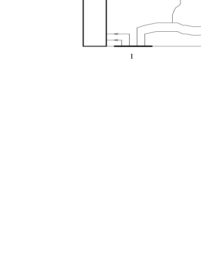
Figure 6: A dirty Hall bar (i.e., $V\neq 0$) in contact with two reservoirs $A$ and $B$ kept at chemical potentials $\mu_{A}$ and $\mu_{B}$. Four contacts have been added as in Fig. 5.

of the problem under a change of direction of the magnetic field, $\vec{B}\to-\vec{B}$, there is only one reflection and transmission coefficient, and not two as in the more general case. We write down the balance equations,

$$I_{A} = {{e^{2}}\over h}\left((N+1)V_{A}-(N+1)V_{1}\right)\;,$$ (71)

$$I_{B} = {{e^{2}}\over h}\left((N+1)V_{B}-(N+1)V_{4}\right)\;,$$ (72)

$$I_{1} = {{e^{2}}\over h}\left((N+1)V_{1}-(N+T)V_{2}-RV_{3}\right)\;,$$ (73)

$$I_{2} = {{e^{2}}\over h}\left((N+1)V_{2}-(N+1)V_{B}\right)\;,$$ (74)

$$I_{3} = {{e^{2}}\over h}\left((N+1)V_{3}-(N+1)V_{A}\right)\;,$$ (75)

and

$$I_{4}={{e^{2}}\over h}\left((N+1)V_{4}-(N+T)V_{3}-RV_{2}\right)\;.$$ (76)

The experimental configuration that allows one to measure the longitudinal and Hall resistances is one where

$$I_{1}=I_{2}=I_{3}=I_{4}=0\;.$$

It immediately follows that

$$I_{A}=-I_{B}=I\;.$$

We now choose one of the six potentials equal to zero, e.g. $V_{B}=0$, to anchor the voltage scale. Equations (71) – (76) may then be transformed into

$$I = {{e^{2}}\over h}(N+T)V_{A}\;,$$ (79)

$$V_{1} = {{e^{2}}\over h}{{R}\over{N+1}}V_{A}\;,$$ (80)

$$V_{2} = 0\;,$$ (81)

$$V_{3} = {{e^{2}}\over h}V_{A}\;,$$ (82)

and

$$V_{4}={{e^{2}}\over h}{{N+T}\over{N+1}}V_{A}\;.$$ (83)

We may now determine the resistances between all pairs of contacts:

$$R_{34}={{V_{3}-V_{4}}\over{I}} = {h\over{e^{2}}}{{R}\over{(N+1)(N+T)}}\;,$$ (84)

$$R_{12}={{V_{1}-V_{2}}\over{I}} = {h\over{e^{2}}}{{R}\over{(N+1)(N+T)}}\;,$$ (85)

$$R_{42}={{V_{4}-V_{2}}\over{I}} = {h\over{e^{2}}}{{1}\over{(N+1)}}\;,$$ (86)

$$R_{31}={{V_{3}-V_{1}}\over{I}} = {h\over{e^{2}}}{{1}\over{(N+1)}}\;,$$ (87)

$$R_{41}={{V_{4}-V_{1}}\over{I}} = {h\over{e^{2}}}{{N-1-2T}\over{(N+1)(N+T)}}\;,$$ (88)

and

$$R_{32}={{V_{3}-V_{2}}\over I}={h\over{e^{2}}}{{1}\over{(N+1)}}\;.$$

If now $T=1$ and $R=0$, which is the case when there is no path across the sample at the Fermi level, Eqs. (84) to (89) reduce to

$$R_{12}=R_{34}=0\;,$$

and

$$R_{42}=R_{31}=R_{41}=R_{32}={h\over{e^{2}}}{1\over{N+1}}\;.$$

This is the integer quantum Hall effect, and we recognize Eqs. (69) and (70) in the last two equations.

From Eqs. (84) to (89) we also see what happens when the system moves from one Hall plateau, i.e., when Eqs. (90) and (91) reign, to the next: A longitudinal resistance appears, as long as $R=1-T>0$. This is the localization-delocalization transition that appears in the Introduction to this article. And, we see now what causes it, namely the appearance of paths across the sample in the $y$ direction at the Fermi level. But, what kind of transition is this? In the early eighties it was suggested that it is the same mechanism as that of coalescing ponds during rainy weather, i.e., it is a percolation transition, see Kazarinov and Luryi [27] and Trugman [28]. However, as has now become clear, this picture was too simple minded.

4. The Critical Points

After having set the scene, we are now ready to discuss the phenomenon which is the aspect of the integer quantum Hall effect that forms the focus of this review: The critical behavior associated with changing the quantized filling factor from $N$ to $N\pm 1$.

4.1 Expectations and Observations

As stated at the end of Sec. 3, it was early theorized that the critical behavior is that of “standard” percolation. The theory goes as follows:

There are three classes of electron wave functions in the system: (i) Wave functions localized to closed paths that follow the sides of “valleys” in the energy landscape $V$, (ii) those localized to closed paths circling the “mountains”, and (iii) those localized to the group of paths that consists of paths of type (i) or (ii) and which are connected through saddle points. For one particular level $V({\vec{x}})=constant$, there is at least one connected cluster of paths (i.e., a separatrix of type (iii)) that spans the system, connecting opposite edge states. The corresponding energy level we denote $E_{c,n}$. As explained in Sec. 3.2, a longitudinal conductance appears each time the Fermi level passes through an $E_{c,n}$ by for example adjusting the perpendicular magnetic field $B$. There is a particular magnetic field $B_{c,n}$ corresponding to the energies $E_{c,n}$.

The typical (linear) size of area the connected wave functions span, $\xi_{p}$, diverges as

$$\xi_{p}\propto|E-E_{c,n}|^{-\nu}\propto|B-B_{c,n}|^{-\nu}\;,$$

where the percolation connectivity length exponent $\nu$ is known to be $4/3$ in two dimensions. The localization length, $\xi$, is the length scale over which the wave function does not fall off faster than algebraically, and behaves as

$$\xi\propto|E-E_{c,n}|^{-\tilde{\nu}}\;,$$

where $\tilde{\nu}$ is the localization length exponent. If percolation, in the sense described above, were the only mechanism, we would have

$$\tilde{\nu}=\nu={4\over 3}\;,\quad{\rm wrong!}$$

This, however, is not what is observed in experiments, nor in computer simulations. Koch et al. [29,30] measured $\tilde{\nu}=2.3\pm 0.1$, while Wei al. [31,32] found the value $\tilde{\nu}=2.4\pm 0.2$. This value was not measured directly, but relies on assumed values of other exponents. On the other hand, Shashkin et al. [33,34] and Dolgopolov et al. [35] observe $\tilde{\nu}\approx 1$, which is not too far from the percolation value $\nu=4/3$. However, also in these three latter papers, $\tilde{\nu}$ was not measured directly, but relied on theoretical arguments.

Several numerical simulations have been performed to determine $\tilde{\nu}$. Models based on continuum descriptions of the problem, using long-wavelength Gaussian potentials or short-range impurity potentials, result in $\tilde{\nu}\approx 2.3$ – 2.4 [36–41].

Network models, originally introduced by Chalker and Coddington [42] give a similar value for $\tilde{\nu}$, see [43,44]. We describe these network models in detail in Sec. 5.

These for the most part mutually consistent results strongly hint at the localization-delocalization transition not being describable by classical percolation alone. Quantum effects play a rôle.

There are two ways that quantum mechanics may change the universality class of the transition, while still keeping the physical picture developed in the preceeding sections of this review and leading to the percolation picture just presented: 1) Tunneling at the saddle points and 2) interference at the saddle points, making this an example of Anderson localization.

4.2 The Mil’nikov and Sokolov Argument

There is a famous argument, first presented by Mil’nikov and Sokolov [20], that leads to

$$\tilde{\nu}=\nu+1={7\over 3}\;,$$

based on purely semi-classical reasoning, i.e., taking only tunneling into account while ignoring interference.

We follow first Hansen and Lütken [45] in their interpretation of the Mil’nikov–Sokolov argument. A different approach, which we also sketch, can be found in Zhao and Feng [46].

Let us assume that there is a typical distance $a$ between saddle points. We tune the magnetic field, and find classical overlap at saddle points in a window $\Delta B$ around $B_{c,n}$ which creates a connected cluster across the sample. Tunneling changes the question of overlap: Overlap is then no longer characterized as overlap within the magnetic length $l$, but by the tunneling probability $T$ given by Eqs. (58) and (59). Let us write Eq. (59) as

$$P=e^{-1/\chi}\;,$$

where

$$\chi={{ml^{2}\sqrt{\alpha\beta}}\over{he|\Delta B|}}\;.$$

Classically, we may define an “elementary” localization length as the typical distance between saddle points, $a$. This is the length over which the electrons may move if there are no overlaps at the saddle points, as they are constrained to follow closed paths with this average diameter.

When tunneling is included, the elementary localization length is changed. When $\Delta B$ is small, we have from Eqs. (58) and (97) that $T\approx e^{-1/\chi}$. An electron starting somewhere in the system will pass $K$ such saddle points with a probability $e^{-K/\chi}$ (when interference effects are ignored). Fixing this probability to, say, $e^{-1}$, we may define a tunnel length to be

$$\Lambda=Ka=\chi a\;.$$

From Eq. (97) we see that $\Lambda\sim|\Delta B|^{-1}$ when $B\to B_{c}$. In terms of the percolation picture, $\Lambda$ takes over from $a$ as the lower cutoff in length scale when tunneling is taken into account, an assumption relying on the one-dimensional character of the percolation clusters near threshold. The percolation correlation length $\xi$ is essentially the size of the largest cluster of connected ribbons. Measured in units of the effective elementary localization length, $\Lambda=\chi a$, $\xi$ diverges as

$${{\xi}\over{\Lambda}}={{\xi}\over{\chi a}}\sim|\Delta B|^{-\nu}\;,$$

as relative to this length, the problem is that of “ordinary” percolation. However, measured relative to a fixed length, such as $a$, one has that

$${{\xi}\over{a}}\sim|\Delta B|^{-(\nu+1)}=|\Delta B|^{-\tilde{\nu}}\;,$$

and Eq. (95) follows.

Equation (99) implies that tunneling increases the localization length in comparison to classical percolation, i.e.,

$$\xi>\xi_{p}\;.$$

However, Zhao and Feng [46] argues that

$$\xi\ll\xi_{p}\;.$$

Their argument goes as follows: We are close to, but not at the classical percolation threshold, and have no infinite cluster yet. The largest cluster of connected paths that would emerge at the percolation threshold has therefore been broken up into islands of size $\xi_{p}$. Between each island there is a saddle point where tunneling is necessary. The system has a width $W$, and therefore the number of such tunneling saddle points is $W/\xi_{p}$. The probability that an electron tunnels through all these saddle points along a path crossing the sample is therefore

$$P_{W}=P^{W/\xi_{p}}=e^{-W/(\xi_{p}\chi)}=e^{-W/\xi}\;,$$

where we have used Eq. (96). The right hand expression defines the localization length, and we find

$$\xi=\chi\xi_{p}\sim|\Delta B|^{-(\nu+1)}\;.$$

We have here used Eqs. (92) and (97). From Eq. (97), we see that a tunnel length scale may be defined,

$$l_{t}=\sqrt{{he|\Delta B|}\over{m\sqrt{\alpha\beta}}}\;,$$

and Eq. (104) may be written

$$\xi=\xi_{p}\left({l\over{l_{t}}}\right)^{2}\;.$$

Since tunneling has been assumed to be the dominating mechanism for transfer across the saddle point, one must have

$$l_{t}\gg l\;.$$

Combination of this inequality with Eq. (106) leads to the inequality (102). It should be noted here that as $|\Delta B|\to 0$, this argument implies a crossover to classical percolation behavior when $l_{t}$ becomes of the order of $l$. More detailed analytical arguments [48] have been constructed that support the rescaling argument in one dimension, but not in two dimensions, which is our concern here. On the other hand, no crossover as implied by the argument basic to Eq. (106) is found in numerical work.

In the above arguments, quantum interference has been left out. It would lead to an Anderson-type localization [1]. There are no arguments on the level of the Mil’nikov-Sokolov that predicts a value for the localization length exponent $\tilde{\nu}$ based on interference. In order to investigate the implications of this mechanism, numerical studies are required. We therefore now turn to the numerical modelling of the integer quantum Hall problem.

5. Numerical Models

In this Section, we turn to the numerical studies of the integer quantum Hall effect. Since Mil’nikov-Sokolov-type argumentation is controversial, and no arguments taking the full quantum mechanical formulation into account that are capable of pinning down the value of $\tilde{\nu}$, it seems that the computer will continue to be the principal tool for studying this problem. The use of numerical methods has, indeed, been quite successful in this field. Not only have results found in experiments been well reproduced on the computer, but also computer results have had predictive power. For example, the Chalker-Coddington model [42], which we will be studying in a moment, predicted in 1988 the value $\tilde{\nu}=2.5\pm 0.5$, while the experimental result $\tilde{\nu}=2.3\pm 0.1$ of Koch et al. [29], was reported three years later.

5.1 The Chalker-Coddington Model

We will in this review concentrate on network models based on the one introduced by Chalker and Coddington [42], as it seems that these models capture very well the critical

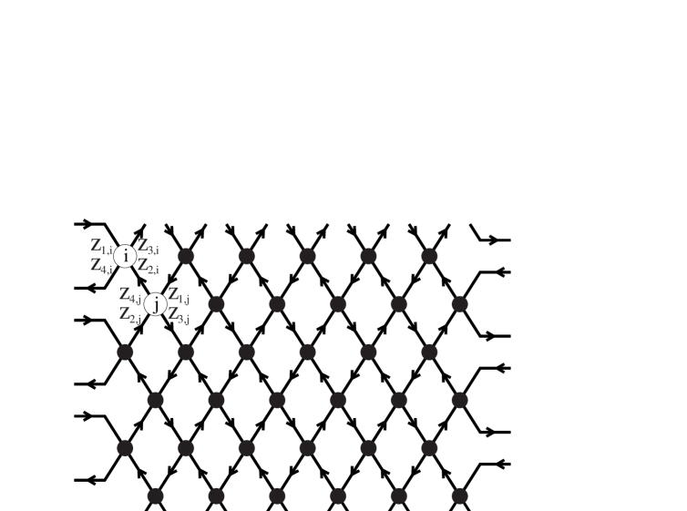
Figure 7: Network used in the Chalker-Coddington model. It has length $L$ in the horizontal direction and length $M$ in the vertical direction. It is periodic in the vertical direction. The amplitudes associated with nodes $i$ and $j$ are shown.

aspects of the integer quantum Hall effect. Other models may be found in Huckestein’s review [13].

The Chalker-Coddington model replaces the random network of paths in the disordered energy landscape by a regular square lattice with a lattice constant equal to the average distance between saddle points in the disordered energy landscape. The nodes of the lattice represent saddle points, and the bonds the paths between the saddle points. Each bond can only be traversed in one direction. The possible directions are chosen so that the network forms a grid of loops of alternating handedness, see Fig. 7. The wave function itself is represented by a complex variable $z$. At a given saddle point, $z_{1}$ and $z_{2}$ are ingoing amplitudes, and $z_{3}$ and $z_{4}$ outgoing amplitudes as shown in Fig. 8. The scattering matrix is conventionally written [42]

$$\left(\matrix{z_{1}\cr z_{3}\cr}\right)=\left(\matrix{e^{i\phi_{1}}&0\cr 0&e^{i\phi_{2}}\cr}\right)\ \left(\matrix{\cosh\gamma&\sinh\gamma\cr\sinh\gamma&\cosh\gamma\cr}\right)\ \left(\matrix{e^{i\phi_{3}}&0\cr 0&e^{i\phi_{4}}\cr}\right)\ \left(\matrix{z_{4}\cr z_{2}\cr}\right)\;.$$

where $\phi_{1}$, $\phi_{2}$, $\phi_{3}$ and $\phi_{4}$, represent the phase changes of the wave function along the bonds. These are chosen at random. This randomness represents the variation in path length from loop to loop. The control parameter $\gamma$ determines the scattering properties at the saddle point. When $\gamma\to 0$,

Figure 8: Scattering at a given node in the Chalker-Coddington model: a) shows the case when $\gamma\leq\gamma_{c}$ while b) shows the case $\gamma\geq\gamma_{c}$. The dashed curves denote the case $\gamma=\gamma_{c}$.

the transmission probabilities are $P_{1\to 4}=P_{2\to 3}=1$ and $P_{1\to 3}=P_{2\to 4}=0$. Likewise, when $\gamma\to\infty$, we have that $P_{1\to 3}=P_{2\to 4}=1$ and $P_{1\to 4}=P_{2\to 3}=0$. When $\gamma=\gamma_{c}=\ln(1+\sqrt{2})$, one finds $P_{1\to 4}=P_{1\to 3}=P_{2\to 4}=P_{2\to 3}=1/2$. When $\gamma<\gamma_{c}$, $P_{1\to 3}=P_{2\to 4}=1/(1+\sinh^{-2}\gamma)$ are due to tunneling, while $P_{1\to 4}=P_{2\to 3}=1-P_{1\to 3}$ are direct channels. When $\gamma>\gamma_{c}$, $P_{1\to 4}=P_{2\to 3}=1/(1+\sinh^{+2}\gamma)$ are due to tunneling while the two remaining channels are direct. This is illustrated in Fig. 8. Writing $P$ as in Eq. (96), derived in the energy landscape model, we may combine all these results in the expression

$$\chi={1\over{2|\ln\sinh\gamma|}}\;.$$

While Chalker and Coddington [42] kept $\gamma$ equal for all nodes, with disorder in the phases $\phi_{i}$ only, Lee et al. [43] extended the original model by writing

$$\gamma=\gamma_{c}e^{\mu-v}\;,$$

thereby introducing disorder also in the saddle points in addition to the one already present. Here $\mu$ is a fixed parameter, equal for all nodes in the network, while $v$ is chosen randomly on the interval $[-w/2,+w/2]$, where $w$ is a parameter determining the width of the distribution. As we will see in Sec. 5.2, the Chalker-Coddington model crosses over to classical behavior in the limit $w\to\infty$. In the case when $|\mu-v|\ll 1$, we may relate $|\mu-v|\propto|B-B_{c}|$ of the energy landscape model. By using Eq. (98) combined with Eqs. (109) and (110), we find that the tunnel length $\Lambda$ behaves as

$$\Lambda=\chi a\propto{a\over{|\mu-v|}}\;,$$

with $a$ the lattice constant. This expression should be compared to the corresponding expression, Eq. (97), derived in the smooth-potential model. Thus, the renormalization argument presented in Sec. 4.2, predicts the same critical behavior in the Chalker-Coddinton model as in the energy landscape model. However, we reiterate that a localization length exponent $\tilde{\nu}=2.35\pm 0.03$ [39] is found in the Chalker-Coddington model without nodal disorder. This has been investigated further, with the conclusion that the Chalker-Coddington model does not support the Mil’nikov and Sokolov argument [49].

The way one determines $\tilde{\nu}$ in the Chalker-Coddington model is based on a transfer matrix approach and the assumtion of one-parameter scaling [50]. The procedure is as follows. The lattice employed is as shown in Fig. 7, but with horizontal length $N$ and vertical length $M$. We assume $N\gg M$ — typically $M$ is of the order of $10^{2}$ and $N$ of the order $10^{5}$. Calculate the trace of the transmission probability from layer one to layer $N$, ${\rm tr}|T|^{2}$. Average this quantity geometrically over the different samples, i.e., calculate $\exp[\langle\ln{\rm tr}|T|^{2}\rangle]$. The reason for doing the geometric average is that we want the typical transmission probability. This is not accessible with the usual arithmetic average, $\langle{\rm tr}|T|^{2}\rangle$, which is dominated by the rare events where the sample actually percolates in the classical sense from edge to edge (in the $M$ direction), and in which case ${\rm tr}|T|^{2}$ is equal to one. In taking the logarithm, these rare events no longer play a rôle. We may now define an effective quantum localization length, $\xi_{M}$ by

$${1\over{\xi_{M}}}=-\lim_{N\to\infty}{1\over N}\ \langle\ln{\rm tr}|T|^{2}\rangle\;.$$

It is effective in the sense that it depends on $M$. The asymptotic localization length, which is the one we want to determine, is then

$$\xi=\lim_{M\to\infty}\xi_{M}\;.$$

At this point, the one-parameter scaling assumption comes into play. It assumes the following functional relationship between $\xi$ and $\xi_{M}$ with $M$ and $\mu$, defined in Eq. (110), as parameters:

$${{\xi_{M}}\over M}=F\left({{\xi(\mu)}\over M}\right)\;.$$

By plotting $\xi_{M}$ for several values of $\Delta B$ and $M$, data collapse is obtained when the correct functional dependence of $\xi$ on $\Delta B$ has been found — which is a power law with slope $-\tilde{\nu}$.

We shall not discuss the basis for the above procedure here, but instead turn to a different way of extracting the localization length exponent from the Chalker-Coddington model. One recently employed consists in treating the network as an open system [51]. By open, we mean the following: Rather than calculating transmission and reflection coefficients from the elementary scattering matrices of Eq. (108), we “hook” the network up to a source and a sink. That is, we specify the value of $z$ on all bonds on the edges leading into the network, while leaving the $z$ values of the exiting bond unspecified. This corresponds to driving a current through the network, and $z$ must now be interpreted as current amplitudes rather than wave functions, as it is no longer normalized. In fact, this models the dirty Hall bar with reservoirs shown in Fig. 6, although the boundary conditions in the transverse direction are different. $\tilde{\nu}$ can then be determined as is done in connection with the classical random resistor network at the percolation threshold.

When the system is considered open, the various link amplitudes are found by solving a set of linear equations,

$$Az=b\;,$$

where $B$ contains the $z$ values that correspond to specified bonds, and the matrix $A$ contains the detailed scattering conditions for each node, based on Eq. (108). We fix all currents entering the network shown in Fig. 7 from the left to unity, while no currents enter the network from the right. By solving Eq. (115), we determine all $z$-values in the network, and from these the total current passing through the system, namely,

$$I=\sum_{i\ \in\ {\rm first\ column}}\left(|z_{1,i}|^{2}-|z_{4,i}|^{2}\right)=\sum_{i\ \in\ {\rm last\ column}}|z_{3,i}|^{2}\;.$$

The first of the two lower indices on the bond variables $z$ refers to the scattering channel as shown in Fig. 7, while the second index is the node address.

The total current entering the network from the left, $I_{l}$ is proportional to the chemical potential of the reservoir hooked up to the network on that side, while the chemical potential on the right is zero, as no current enters from this side. Thus, the potential difference across the network is simply $V=h/e^{2}I_{l}$. We may now define a longitudinal conductance $G$ through the expression

$$I=VG\;.$$

As is evident from Fig. 7, the nodes belonging to every second row have their scattering labels rotated by $90^{\circ}$ in the clockwise direction. As a result of this rotation, the connection between bond labels and forward/backward scattering depends on which row the nodes belong to. For the odd-numbered rows, scattering $z_{1}\to z_{3}$ represents forward scattering, whereas for the even rows, it is represented by $z_{2}\to z_{3}$. The scattering amplitude for channel $z_{1}\to z_{3}$ increases with increasing $\gamma$, whereas the scattering amplitude for channel $z_{2}\to z_{3}$ increases with decreasing $\gamma$.

Rather than assigning random values for $\gamma$ to the nodes in the network, we have used two bimodal distributions, one for the odd rows,

$$p_{o}(\gamma)=(1/2+\mu)\delta(\gamma-\gamma_{13})+(1/2-\mu)\delta(\gamma-\gamma_{23})\;,$$

and one for the even rows,

$$p_{e}(\gamma)=(1/2-\mu)\delta(\gamma-\gamma_{13})+(1/2+\mu)\delta(\gamma-\gamma_{23})\;.$$

These two distributions contain three parameters: $\gamma_{13}$, $\gamma_{23}$ and $\mu$. We relate $\gamma_{13}$ and $\gamma_{23}$ through the relation

$$\tanh\gamma_{13}={1\over{\cosh\gamma_{23}}}=t_{0}\;,$$

where $t_{0}$ is a transmission amplitude. With the relation (120), a node belonging to an even row with a $\gamma=\gamma_{23}$ will transmit in exactly the same manner as a node belonging to an odd row with $\gamma=\gamma_{13}$. When $|t_{0}|\to 1$, tunneling becomes less and less likely and the model becomes classical, as will be discussed in Sec. 5.2. On the other hand, in the $|t_{0}|\to 1/\sqrt{2}$ limit we find that $\gamma_{13}=\gamma_{23}=\gamma_{c}=\ln(1+\sqrt{2})$.

With a large negative value of control parameter $\mu$, the system will predominantly consist of elementary loops with current running clockwise, whereas with a large positive value of $\mu$, the current will be running counterclockwise in loops shifted by one lattice constant in the (11) direction. When $\mu=0$, there is no bias and the system is critical.

In our simulations, we set $t_{0}=0.9$, and let $\mu$ vary between -0.5 and 0.5. In Fig. 9 we show the current $I$ as a function of $\mu$ for square system sizes $L=12$ to 92. The data were geometrically averaged over 14650 samples for $L=12$ to 300 samples for $L=92$.

From Fig. 9 we see that the larger the system size, the sharper the peak. The system becomes critical when $L/\xi(\Delta\mu)\simeq 1$, hence we find that the half width, $\Delta\mu$, scales as

$$\Delta\mu\propto L^{-1/\tilde{\nu}}\;.$$

By plotting the half width $\Delta\mu$ versus system size in a log-log plot, Fig. 10, we obtain the localization length exponent $\tilde{\nu}=2.35\pm 0.07$.

So far, we have only discussed one single critical exponent associated with the localization-delocalization exponent in the quantum Hall effect, namely $\tilde{\nu}$, the localization length exponent. Recent analysis of the Chalker-Coddington model by Klesse and Metzler [54], which is based on earlier work of Pook and Janßen [55], shows that the wave function is multifractal in this model. In terms of an open system, where $z$ is to be interpreted as a current amplitude, the problem is operationally analogous to the random resistor network at the percolation threshold, where it also has been established that the current distribution is multifractal [56,57].

Figure 9: The current passing through the system as a function of chemical potential, for various system sizes.

Multifractality means the following: At the critical point, the logarithmically binned histogram, $H$, of currents $z$ show the following scaling form:

$$H(z,L)\sim L^{f(\alpha)}\;,$$

where

$$z\sim L^{-\alpha}\;,$$

and $L$ is the lattice size (assuming a square lattice). The two functions $f$ and $\alpha$ are independent of $L$. If $f(\alpha)$ is a more complicated function of $\alpha$ than of linear form $a+b\alpha$, then the current distribution is multifractal. This signifies that there is a continuum of singularities governing the distribution — singularities in the sense of non-trivial power laws, and not just a small number of exponents, which is usually the case in connection with critical phenomena. The geometrical scaling properties of percolation, for example, are completely described by two exponents, while the current distribution is multifractal.

Figure 10: Log-log plot of the half width of the curves shown in Fig. 9. The straight line is the result of a least squares fit giving $\tilde{\nu}=2.35\pm 0.07$.

One can study a distribution by building a histrogram. Equivalently, one can explore it by measuring its moments. In our case, we define the $n$th current moment as

$$M_{n}=\langle\sum_{i}|z|^{2n}\rangle\sim L^{y(n)}\;.$$

They all turn out to scale as power laws. The tell-tale sign of multifractality is that

$$y(n)\neq y(0)+cn\;,$$

where $c$ is a constant. The fundamental relation between $f$, $\alpha$, $y$ and $n$ is of the Legendre type,

$$y(n)=f-n\alpha\;.$$

This interpretation and equation form the heart of the celebrated $f-\alpha$ formalism [58].

We will not pursue this line any further here, except for pointing out that this is today an active field of research.

Figure 11: The Chalker-Coddingon model in the limit $w\to\infty$ generates “dragon curves” by randomly tiling the plane with the two Truchet tiles shown.

5.2 Classical Limit of the Chalker-Coddington Model

The Chalker-Coddington model has an interesting classical limit. For finite $\mu$ and $v\to\infty$, defined in Eq.  (110), the scattering channels are $z_{1}\to z_{4}$ and $z_{2}\to z_{3}$, and when $v\to-\infty$ they are $z_{1}\to z_{3}$ and $z_{2}\to z_{4}$. In this extreme case, there is no contact across the saddle points. However, delocalization is still possible. The localization length exponent in the extreme case when $w\to\infty$ has been measured by Lee et al. [43] to be $1.29\pm 0.05$ in agreement with classical percolation theory (predicting 4/3). However, Bratberg et al. [51] have noted that the system in this limit is not equivalent to the percolation picture presented in Sec. 4, but to the system shown in Fig. 11. This is a random tiling of the two elements shown at the bottom of the figure. The curves that the markings on the tilings — known as Truchet tiles, see e.g. Gale [59] — produce are known as Dragon curves, see Wells [60]. The critical properties of this tiling was studied some time ago by Roux et al. [61]. Their conclusion was that it is in the universality class of smart kinetic walks (SKW). These may be mapped on the external perimeters of percolation clusters in two dimensions. As a consequence, their correlation length exponent is the same as in percolation: $\nu_{SKW}=\nu=4/3$. Thus, the Chalker-Coddington model with its good exponent $\tilde{\nu}=2.35\pm 0.03$, does not simulate the percolation picture of the localization-delocalization transition in the integer quantum Hall system in the “classical” limit, $w\to\infty$, where $w$ is the width of the distribution from which $v$ is chosen. The criticality of the model in this limit comes from the loop size distribution, and not from joining of overlapping loops at saddle points, as there are no saddle point crossings.

6. Conclusion

We summarize in a few sentences the picture of the integer quantum Hall effect that we have presented here. Non-interacting electrons move two-dimensionally in a strong perpendicular magnetic field and in a disordered potential. Classically, the perpendicular magnetic field causes the electrons to move in circles about the so-called “guiding centers.” Quantum mechanically, this circular motion is quantized into Landau levels. We assume the disorder potential to be slowly varying on the scale of the radii of the Landau levels, so that there are no transitions between these caused by the potential. The Schrödinger Eq. (45) then simplifies to Eq. (49), which shows that the energetically allowed regions where the electron may move are the equipotential curves of the disordered potential. The wave function is localized to bands of width of the order of the radius of the Landau level, and follows the equipotential curves of the potential. By adjusting the perpendicular magnetic field, these curves move up or down in the disordered potential landscape. At a particular critical value of the magnetic field, there will be a continuous path of equipotential curves that span the system. The electrons in this Landau level are then delocalized, and there is longitudinal conductance. For other values of the magnetic field, they are not. This mechanism is repeated for every filled Landau level up to the Fermi level. The localization-delocalization transition is driven by coalescence of disjoint equipotential curves, and strongly resembles classical percolation. However, tunneling at the saddle points and interference effects change the universality class of the transition from that of percolation. There are semi-classical arguments that reproduce the delocalization length exponent seen numerically and experimentally, which essentially describe the localization-delocalization transition as a “dressed” percolation process. However, these arguments have serious weaknesses, and it seems likely that the transition is a pure quantum one.

The number of experiments that directly test the scaling properties of the transition are few and to a certain degree not consistent with each other. Why do for instance Dolgopolov et al. [35] find a localization exponent $\tilde{\nu}\approx 1$ which is roughly consistent with the classical value $\nu=4/3$, rather than the quantum value $\approx 2.3$? The argument used to derive the exponent $\tilde{\nu}\approx 1$ in the work of Dolgopolov et al. [34] is equivalent to the gradient percolation argument of Sapoval et al. [62], which is in fact incompatible with the slowly-varying landscape model presented in these lectures.

This is clearly not a closed subject.

7. Acknowledgements

We thank I. Bratberg, J. Hajdu, J. S. Høye, B. Huckestein, M. Janßen, J. Kertész, R. Klesse, J. M. Leinaas, C. A. Lütken, M. Metzler, J. Myrheim, K. Olaussen, J. Piasecki and D. Polyakov for discussions. This work was in part supported by the Norwegian Research Council. A.H. furthermore thanks J. Hajdu and SFB 341 for an invitation to Cologne where part of this review was written.

References

[1] P. W. Anderson, Phys. Rev. 109, 1492 (1958).

[2] P. W. Anderson in Les Prix Nobel 1977 (Almqvist and Wiksell, Stockholm, 1978).

[3] P. J. Flory, J. Am. Chem. Soc. 63, 3083 (1941); ibid 63, 3091 (1941).

[4] A. S. Skal and B. I. Shklovskii, Sov. Phys. Semicond. 8, 1029 (1974).

[5] M. Sahimi in Annual Review of Computational Physics, Vol. II, ed. by D. Stauffer (World Scientific, Singapore, 1995).

[6] D. J. Thouless in Ill-condensed Matter, ed. by R. Balian, R. Maynard and G. Toulouse (North-Holland, Amsterdam, 1979).

[7] N. W. Ashcroft and N. D. Mermin, Solid State Physics (Saunders Collegem Philadelphia, 1976).

[8] K. von Klitzing, G. Dorda and M. Pepper, Phys. Rev. Lett. 45, 494 (1980).

[9] M. A. Paalanen, D. C. Tsui and A. C. Gossard, Phys. Rev. B 25, 5566 (1982).

[10] R. E. Prange and S. M. Girvin, The Quantum Hall Effect (Springer Verlag, Berlin, 1987).

[11] M. Janßen, O. Vieweger, U. Fastenrath and J. Hajdu, Introduction to the theory of the integer quantum Hall effect (VCH, Weinheim, 1994).

[12] T. Chakraborty and P. Pietiläinen, The quantum Hall effects (2nd ed., Springer, Heidelberg, 1995).

[13] B. Huckestein, Rev. Mod. Phys. 67, 357 (1995).

[14] R. Kubo, S. J. Miyake, N. Hashitsume, Solid State Physics 17, 269 (1965).

[15] M. Tsukada, J. Phys. Soc. Japan, 41, 1466 (1976).

[16] W. Gröbli, Vierteljahrschrift der Naturforschenden Gesellschaft in Zürich, 22, 37, (1877); ibid 22, 129 (1877).

[17] J. L. Synge, Can. J. Phys. 26, 257 (1948).

[18] H. Aref, Phys. Fluids 22, 393 (1979).

[19] H. A. Fertig, Phys. Rev. B 38, 996 (1988).

[20] G. V. Mil’nikov and I. M. Sokolov, JETP Letters 48, 536 (1988).

[21] A. Hansen, Springer Lect. Notes on Physics, 437, 331 (1994).

[22] D. ter Haar, Selected Problems in Quantum Mechanics (Infosearch, London, 1964).

[23] L. D. Landau and E. M. Lifshitz, Quantum Mechanics (Pergamon, Oxford, 1965).

[24] M. Büttiker, Phys. Rev. Lett. 57, 1761 (1986).

[25] B. I. Halperin, Phys. Rev. B 25, 2185 (1982).

[26] M. Büttiker, Phys. Rev. B 38, 9375 (1988).

[27] R. F. Kazarinov and S. Luryi, Phys. Rev. B 25, 7626 (1982).

[28] S. A. Trugman, Phys. Rev. B 27, 7539 (1983).

[29] S. Koch, R. J. Haug, K. von Klitzing and K. Ploog, Phys. Rev. Lett. 67, 883 (1991).

[30] S. Koch, R. J. Haug, K. von Klitzing and K. Ploog, Phys. Rev. B 46, 1596 (1992).

[31] H. P. Wei, D. C. Tsui, M. A. Paalanen and A. M. M. Pruisken, Phys. Rev. Lett. 61, 1294 (1988).

[32] H. P. Wei, L. W. Engel and D. C. Tsui, Phys. Rev. B 50, 14609 (1994).

[33] A. A. Shashkin, V. T. Dolgopolov and G. V.  Kravchenko, Phys. Rev. B 49, 14486 (1994).

[34] A. A. Shashkin, V. T. Dolgopolov, G. V. Kravchenko, M. Wendel, R. Schuster, J. P. Kotthaus, J. R. Haug, K. von Klitzing, K. Ploog, H. Nickel and W. Schlapp, Phys. Rev. Lett. 23, 3141 (1994).

[35] V. T. Dolgopolov, A. A. Shashkin, G. V. Kravchenko, C. J. Emeleus and T. E. Whall, JETP Letters, 62, 168 (1995).

[36] B. Mieck, Europhys. Lett. 13, 453 (1990).

[37] B. Huckestein and B. Kramer, Phys. Rev. Lett. 64, 1437 (1990).

[38] Y. Huo and R. N. Bhatt, Phys. Rev. Lett. 68, 1375 (1992).

[39] B. Huckestein, Europhys. Lett. 20, 451 (1992).

[40] D. Liu and S. Das Sarma, Phys. Rev. B 49, 2677 (1994).

[41] P. M. Gammel and W. Brenig, Phys. Rev. Lett. 73, 3286 (1994).

[42] J. T. Chalker and P. D. Coddington, J. Phys. C 21, 2665 (1988).

[43] D. H. Lee, Z.  Wang and S. Kivelson, Phys. Rev. Lett. 70, 4130 (1993).

[44] D. K. K. Lee and J. T. Chalker, Phys. Rev. Lett. 72, 1510 (1994).

[45] A. Hansen and C. A. Lütken, Phys. Rev. B 51, 5566 (1995).

[46] H. L. Zhao and S. Feng, Phys. Rev. Lett. 70, 4134 (1993).

[47] A. Coniglio, J. Phys. A 15, 3829 (1982).

[48] A. Hansen and J. Kertész, preprint, 1997.

[49] L. Jaeger, J. Phys. C 3, 2441 (1991).

[50] A. Mackinnon and B. Kramer, Phys. Rev. Lett. 47, 1546 (1981).

[51] I. Bratberg, A. Hansen and E. H. Hauge, Europhys. Lett. 37, 19 (1997).

[52] J. M. Normand, H. J. Herrmann and M. Hajjar, J. Stat. Phys. 52, 441 (1988).

[53] A. Hansen in Statistical Models for the Fracture of Disordered Materials, ed. by H. J. Herrmann and S. Roux (North Holland, Amsterdam, 1990).

[54] R. Klesse and M. Metzler, Europhys. Lett. 32, 229 (1995).

[55] W. Pook and M. Janßen, Z. Phys. B 82, (1991).

[56] R. Rammal, C. Tannous, P. Breton and A. M. S. Tremblay, Phys. Rev. Lett. 54, 1718 (1985).

[57] L. de Arcangelis, S. Redner and A. Coniglio, Phys. Rev. B 31, 4725 (1985).

[58] T. C. Halsey, M. H. Jensen, L. P. Kadanoff, I. Procaccia and B. Shraiman, Phys. Rev. A 33, 1111 (1986).

[59] D. Gale, Math. Intelligencer 17, (3), 48 (1995).

[60] D. Wells, The Penguin Dictionary of Curious and Interesting Geometry. (Penguin, London, 1991).

[61] S. Roux, E. Guyon and D. Sornette, J. Phys. A 21, L475 (1988).

[62] B. Sapoval, M. Rosso and J. F. Gouyet, J. Phys. (France) 46, L149 (1985).