International Journal of Modern Physics C,
c  World Scientific Publishing Company

1

ENTROPY AND CORRELATIONS IN LATTICE GAS AUTOMATA

WITHOUT DETAILED BALANCE

OLIVIER TRIBEL

and

JEAN PIERRE BOON

Center for Nonlinear Phenomena and Complex Systems

Université Libre de Bruxelles, Campus Plaine, C.P. 231

1050 Brussels, Belgium

Received (received date)
Revised (revised date)

We consider lattice gas automata where the lack of semi-detailed balance results from node occupation redistribution ruled by distant configurations; such models with nonlocal interactions are interesting because they exhibit non-ideal gas properties and can undergo phase transitions. For this class of automata, mean-field theory provides a correct evaluation of properties such as compressibility and viscosity (away from the phase transition), despite the fact that no $H$-theorem strictly holds. We introduce the notion of locality – necessary to define quantities accessible to measurements – by treating the coupling between nonlocal bits as a perturbation. Then if we define operationally “local” states of the automaton – whether the system is in a homogeneous or in an inhomogeneous state – we can compute an estimator of the entropy and measure the local channel occupation correlations. These considerations are applied to a simple model with nonlocal interactions.

Keywords: Lattice gas automata, $H$-theorem, entropy, correlations.

1 Introduction

Various lattice gas automaton (LGA) models lacking semi-detailed balance (SDB) have been proposed because they exhibit interesting properties for investigating phenomena which are not accessible to LGAs satisfying SDB. LGAs violating SDB locally have been constructed for their operational value as possible candidates for the simulation of high Reynolds number hydrodynamics^?,?,?. Such systems were subsequently reconsidered as a paradigmatic formulation of driven systems^?. The implications and consequences of the lack of semi-detailed balance in lattice gas automata are non-trivial, in particular for what concerns their stationary distribution function and the very existence of an equilibrium distribution for such systems which exhibit thermodynamic properties and transport properties correctly described by mean-field theory. This somewhat paradoxical situation has been the subject of consideration in the recent literature^?,? where the question was raised whether the asymptotic state of systems without SDB can be qualified as an equilibrium state. Certain LGAs without detailed balance were shown to approach a stable uniform state referred to as a non-Gibbsian equilibrium^? with nonlocal spatial correlations, in contrast to the classical Gibbsian state of thermal equilibrium.

The problem has not been examined in depth for the case of LGAs where the lack of SDB results from node occupation redistribution ruled by distant configurations; such models with nonlocal interactions (NLIs) are interesting because they exhibit non-ideal gas properties^? and can undergo phase transitions^?. For this class of LGAs, mean-field theory is also seen to provide a correct evaluation of properties such as compressibility and viscosity^?,? (away from the phase transition) and static correlation functions are in accordance with those observed in real fluids^?. It has even been suggested that a generalized version of the SDB condition could be applicable to recast LGAs with NLIs such that a generalized $H$-theorem would hold^?. The situation calls for clarification, starting at the level of the basic statistical mechanical description of LGAs.

2 Statistical Mechanics

We consider a set ${\cal S}$ of Boolean variables (bits), ${\cal S}=\{s_{(i)},i=1,\ldots,bV\}$ with $s_{(i)}\in\{0,1\}$ (here $bV$ is simply an integer; $b$ and $V$ will be specified subsequently), and an update rule: ${\cal T}_{\lambda}:{\cal S}\rightarrow{\cal S}$, with $\lambda$ a set of parameters, allowing for example ${\cal T}$ to be drawn probabilistically among a set of rules. This update rule is set according to certain constraints which are chosen on the basis of physical requirements. ${\cal S}$ and ${\cal T}$ define the lattice gas automaton. The constraints on ${\cal T}$ are of two types:

• Geometric constraints lead to a spatial representation of the LGA, and impose certain symmetries on this representation. This essentially amounts to defining a set of relations $\{\left(i,\varphi(i)\right),i=1,\ldots,bV\}$ between indices of elements of ${\cal S}$. With these relations, the update rule ${\cal T}_{\lambda}$ may be factorized into several steps, one of which is simply the copying of the value of bit $i$ onto bit $\varphi(i)$; this step is called propagation and the corresponding operator${}^{\mbox{\scriptsize a}}$  is denoted by ${\cal P}$. An important feature of propagation is that it is a mere correspondence between indices of elements of ${\cal S}$, independently of the values taken by these elements. To each $\varphi(i)$ we associate a geometric vector ${\bf c}_{(i)}$ in a suitable space, and these vectors (which may include the null vector) are grouped into $b$ equivalence classes. The vectors representative of these classes will be denoted by ${\bf c}_{i}$ (with $i=1,\ldots,b$); they must satisfy symmetry constraints in order to obtain a consistent geometric representation.

• Conservation laws provide physical content. For example, denote by $n_{(i)}$ the value taken by the variable $s_{(i)}$; then define a quantity $N[{\cal S}]=\sum_{i=1}^{bV}n_{(i)}$, which is identified as the number of particles, and demand that $N[{\cal T}_{\lambda}{\cal S}]=N[{\cal S}]$. A similar conservation is generally required for linear momentum ${\bf p}=\sum_{i=1}^{bV}n_{(i)}{\bf c}_{i}$.

We factorize the transformation ${\cal T}_{\lambda}$ as:

$${\cal T}_{\lambda}={\cal P}\circ{\cal U}_{\lambda}$$ (1)

where ${\cal P}$ is the propagation as defined above. Now, through the operator ${\cal U}_{\lambda}$, it may happen that one can define locality . If ${\cal U}_{\lambda}$ is such that there exists a decomposition of ${\cal S}$ into subsets $s._{(x)}$ in such a way that the restriction of ${\cal U}_{\lambda}$ over $s._{(x)}$, denoted by ${\cal U}_{\lambda}|_{s._{(x)}}$, is completely defined and is an endomorphism:

$${\cal U}_{\lambda}|_{s._{(x)}}:s._{(x)}\rightarrow s._{(x)}\,,\;\forall(x)\,,$$

— i.e. if the values taken by the bits of $s._{(x)}$ after application of ${\cal U}_{\lambda}$ are entirely defined by their values before this application — then the set of indices that define the subset $s._{(x)}$ is called a node; the values taken by the bits of $s._{(x)}$ define the state of the node. Given the above definition of $b$, $V$ is now seen to be the number of nodes of the automaton universe and $b$ the number of channels per node. Then one may construct a representation of the bits that belong to a given $s._{(x)}$ as ‘particles’ and ‘holes’ spatially located on the spot defined by $x$. The action of ${\cal U}$ is then local and ${\cal U}$ is called a collision operator (and will be denoted by ${\cal C}$). We call L-subsets the subsets $s._{(x)}$ thus defined. Note that it is not mandatory that a LGA have such a property; for example the models defined in section 3 have an update operator that cannot be decomposed strictly into propagation and collision operators.

2.1 A Liouville $H$-theorem

We denote by $\Gamma$ the set of all possible sets ${\cal S}$. We associate to each universe-state ${\cal S}$ a probability $P({\cal S})$ in a Gibbs ensemble and define a transition probability ${\cal A_{SS^{\prime}}}$ between universe-states, such that the system obeys a Chapman-Kolmogorov equation:

$$P(S^{\prime})=\sum_{{\cal S}\in\Gamma}{\cal A_{SS^{\prime}}}P({\cal S})\,,\;(S^{\prime}\in\Gamma)\,.$$ (2)

The following hypothesis on ${\cal A}$, the semi-detailed balance (SDB) condition:

$$\sum_{{\cal S}\in\Gamma}{\cal A_{SS^{\prime}}}=1,$$ (3)

suffices to prove an $H$-theorem^?; then the global entropy

$$H=-\sum_{{\cal S}\in\Gamma}P({\cal S})\ln P({\cal S})$$ (4)

does not decrease under the action of ${\cal U}$. Furthermore, as noted above, the propagation operator produces a deterministic redistribution of the bits without introducing or removing information; consequently ${\cal P}$ does not modify the value of $H$.

For all practical implementations, $|\Gamma|$ is finite, but so large that no meaningful sampling is realizable; as a result the quantities $P({\cal S})$ and ${\cal A_{SS^{\prime}}}$ are not accessible to significant measurements.

2.2 Locality and nonlocality

If the updating operator ${\cal T}$ is such that it admits a decomposition into a propagation operator ${\cal P}$ and a local collision operator ${\cal C}$, the local subsets $s_{(x)}$ define subspaces $\gamma_{(x)}$ of $\Gamma$, with $\Gamma=\bigotimes_{(x)}\gamma_{(x)}$. If we assume that the $\gamma_{(x)}$’s are isomorphic, then there exist local states $s$ such that the description of the automaton in terms of the $s$’s is equivalent to its description in terms of ${\cal S}$. Those states (of the nodes) are independent of each other for the local operator, so that we can define a local probability $p(s_{(x)})$ in a (smaller) Gibbs ensemble. If the local dynamics is described with a transition probability matrix $A_{ss^{\prime}}$, then under the condition $\sum_{s\in\gamma}A_{ss^{\prime}}=1(s^{\prime}\in\gamma)$, a local $H$-theorem holds^? and the quantity

$$h(x)=-\sum_{s\in\gamma}p[s_{(x)}=s]\ln p[s_{(x)}=s]\equiv-\sum_{s\in\gamma}p(s_{(x)})\ln p(s_{(x)})$$ (5)

does not decrease under the action of ${\cal C}$.

In this local description, the action of ${\cal P}$ is unimportant as it just provides at each iteration a fresh configuration of the bits of $s_{(x)}$ with probability $p(s)$ by definition; this probability is such that $h$ does not decrease. The action of ${\cal P}$ is of importance when one considers the connection between the local entropy (5) and the global entropy (4). If the propagation does not produce correlations between the nodes, then the global entropy $H$ is entirely determined by the local entropy $h$:

$$H=\sum_{x}h(x).$$ (6)

The existence of a notion of locality provides us with objects (the $s_{(x)}$’s) which are accessible to measurements; then we can define the local number of particles $n(x)$ and the local distribution function $\rho(x)$ by averaging $n(x)$ over the appropriate Gibbs ensemble: $\rho(x)\equiv\langle n(x)\rangle$. We may choose the $s$’s as fundamental dynamical objects to which “physical” properties are then associated. In usual LGAs, this is accomplished by imposing constraints such as “mass” and “momentum” conservation. It is only because the update rule allows a definition of locality — i.e. the universe is a set of independent subsets — that such constraints have physical justification since isolated objects can now be considered. The local constraints are chosen according to the problem to be investigated and provide physical significance to the LGA model.

An important point is that the decomposition may be further pursued: we can describe the dynamics in terms of local space-velocity occupation $n_{i}(x)$ – i.e. the value taken by the bit $s_{(x)i}$, with $x=1,...,V$, and $i=1,...,b$ – and of local single-particle space-velocity distribution functions $p[s_{(x)i}=1]=f_{i}(x)\equiv f({\bf x},{\bf c}_{i})$. At this level of description an entropy is defined by:

$$h_{f}(x)=-\sum_{i=1}^{b}[f_{i}(x)\ln f_{i}(x)+\overline{f_{i}(x)}\ln\overline{f_{i}(x)}],$$ (7)

(where $\overline{f_{i}(x)}\equiv 1-f_{i}(x)$) which, under the Boltzmann ansatz, is simply equal to $h(x)$ (5). The second term on the r.h.s of (7) stems from the correlations between “particles”(1-bits) and “holes” (0-bits) because of the Boolean nature of the variables. Omitting this term amounts to neglecting the important contribution of the “particle - hole” correlations to the entropy.

If the operator ${\cal U}$ does not decompose ${\cal S}$ into independent, disjoint subsets, then we have no consistent definition of locality. In particular, we cannot meaningfully define states $s$ and probabilities $A_{ss^{\prime}}$, and we have no definition of objects to which Statistical Mechanics can be applied: the semi-detailed balance condition is void, and no “local” $H$-theorem can exist. An example is the class of automata with “nonlocal interactions” (see section 3). We will however argue that some models have update rules that allow for a weaker definition of locality, i.e. there may exist a collection of disjoint subsets of ${\cal S}$, the bits of which are strongly coupled through ${\cal U}$, but only weakly coupled to the bits of other subsets. We will call these subsets $\ell$-subsets. Then we can operationally define these subsets as objects of Statistical Mechanics, even if they do not contain the full dynamics of the automaton. This is equivalent to ignoring all dependencies and correlations between “nodes”. If the coupling between “nonlocal” bits can be treated as a perturbation, then we may be able to extract significant information on the dynamics via “local” quantities. However some basic elements necessary to establish the validity of mean-field theory (mainly the $H$-theorem) are then absent, and care must be taken in defining and using “standard” quantities.

3 A Simple Model with “Nonlocal Interactions”

An example of a system where semi-detailed balance does not exist is the LGA with “nonlocal interactions” introduced by Appert and Zaleski^?, subsequently analyzed by Gerits et al.^?, and generalized by Tribel and Boon^?. Here we consider an utmost simplified version of the automaton which nevertheless exhibits all essential features and physical properties of the original model.

The LGA is composed of a set of bits (typically 393216) and an update rule ${\cal T}$ as described in Section 2. This rule admits a decomposition into two operators; one of them is the propagation operator ${\cal P}$ which copies the value contained in $s_{(i)}$ onto the bit labeled $\varphi(i)$. The actual computation of $\varphi(i)$ is performed by a computer routine which is described elsewhere^?. The computation procedure exhibits the following features: it defines the topology of the space used for the representation of the state of the automaton on the surface of a torus and it yields six classes of equivalence of the $(i,\varphi(i))$’s to which we associate six vectors ${\bf c}_{i}$; for symmetry reasons these vectors are chosen to be coplanar and normalized. The spatial representation of the lattice therefore has a toroidal topology and a planar geometry, the geometry of a triangular lattice with hexagonal symmetry.

The second operator ${\cal U}$ which together with ${\cal P}$, composes the full updating operator is itself decomposed into two parts:

$${\cal U}={\cal U}_{2}\circ{\cal U}_{1}.$$

${\cal U}_{2}$ groups the bits of ${\cal S}$ by subsets of six, and re-shuffles the bits within the subsets. The grouping is such that, for any $i$ in a given $\ell$-subset $s_{(x)}$, $\varphi(i)$ is in another $\ell$-subset $s_{(x)}$; for the re-shuffling, we use the rules of the FHP-I automaton (the collision outcome is governed by a Boolean parameter)^?. We denote by $s_{(x,j)}$ the $j$-th bit of the subset $s_{(x)}$; since there is a one-to-one correspondence between the indices $(i)$ and the indices $(x,j)$, we may denote by $\varphi(x,j)$ the index of the bit where ${\cal P}$ copies the bit $(x,j)$, and by $\varphi^{k}(x,j)$ the index where $(x,j)$ should be copied by applying $k$ times the operator ${\cal P}$. Finally, we will be interested in the $\ell$-subset to which $\varphi^{k}(x,j)$ belongs; its index will be $\chi(x,j,k)$.

The operator ${\cal U}_{1}$ re-shuffles the bits that belong to different $\ell$-subsets, according to the following procedure:

• draw a random number $D$, with equal probabilities among $\{1,2,3\}$ (corresponding to the three axial directions of the lattice);

• for each subset $s_{(x)}$, draw a random number $r$ according to a given probability distribution (which may be degenerate); then, write the value $n_{(x,j)}$ taken by the bit $s_{(x,j)}$;

• if: $s_{(x,D+1)}=1$, $s_{(x,D+2)}=0$, $s_{(\chi(x,D,r),D+1)}=0$, and $s_{(\chi(x,D,r),D+2)}=1$, then exchange these values such that $0$ becomes $1$ and vice-versa;

• repeat with $D+4$ and $D+5$;

• repeat the last two steps with $D$ replaced by $D+3$.

All the values of $D+E(E=1,...,5)$ are mapped onto $(1,...,6)$. The set of parameters $\lambda$ in $\cal U_{\lambda}$ is formed by the Boolean parameter of the collision, the direction $D$, and the distance $r$ (the set of distances).

This model exhibits a phase transition when $r$ exceeds a given value (or an average value computed over a given probability distribution); away from the transition, the macroscopic properties of the LGA are characterized by well-defined coefficients^?,?.

Figure 1: Estimated entropy, Eq.(8), as a function of time ($t>t^{*}$, see text). FHP automaton with strictly local collision rules and SDB (solid line), and LGA with NLI (interaction distance = 5 lattice units): (i) entropy estimated from the channel distributions $f_{i}$ (indistinguishable from full line), and (ii) entropy estimated from the configuration probability $p(s,t)$ (dashed line). All cases: average density $f=0.1$, lattice size $256\times 256$ nodes, $t^{*}=500$; time unit$=$automaton time step.

Figure 2: Example of transition probabilities yielding a seemingly valid SDB. Left boxes: initial configurations (arrows indicate particles). Right boxes: output configurations (after non-local interaction and collision) with the corresponding probabilities, assuming that the particles on the “pairing nodes” are randomly distributed ($p$ is then simply one-third of the average density). Considering the sum of the transition probabilities with an output configuration where the particle is in the upper right channel (shown as dot-dashed arrow), the sum is clearly equal to one.

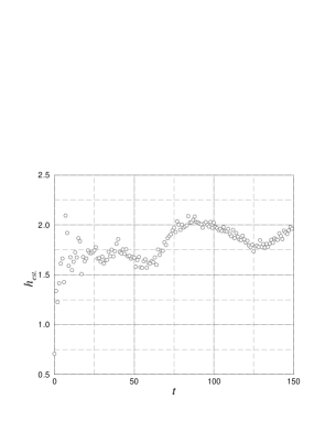
Figure 3: The entropy estimator, evaluated using the occurrence frequency $\nu(s,t)$ of a “local” configuration at a given node of the lattice, for 150 time-steps and 10000 realizations. The system is initialized with a step-function in the density field which is then relaxed; the estimator is measured on a node located at a position along the initial step. Parameters for the simulation: distribution of interaction distances between $1$ and $8$ lattice units, with $p(r)\propto r^{-1}$; initial density: $f=0.1$ on one half of the lattice, $f=0$ on the other half; lattice size $256\times 256$ nodes. No phase transition occurs for these values of the parameters.

Figure 4: Nonlocal channel pair occupation probabilities, evaluated on nodes separated by interaction distance $r$ in LGA with NLI as described in the text. The probabilities $P_{ij}(r,{{\bf c}}_{D})$ are measured along a chosen direction $D$ (here $D=0$) when the interaction between channels labeled $i$ and $j$ occurs along that direction. The black dots are the superposition of data for $i=0\ldots 5$. The density field is homogeneous; parameters of the simulation: $f=0.1$, $r=5$, lattice size $256\times 256$ nodes.

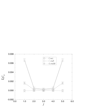
Figure 5: Local channel correlations ($C_{ij}(0)=\langle n_{i}({\bf x})n_{j}({\bf x})\rangle-f^{2}$). Parameters of the simulation: $f=0.1$; lattice size $256\times 256$ nodes; interaction distance $r=5,10$; for comparison the open circles refer to the LGA without NLI.

3.1 Entropy

We may operationally define “local” states $s(x,t)$ ($\ell$-subsets) of the automaton (at time $t$), and, if the LGA is in a homogeneous state, we can evaluate the occurrence probability $p(s,t)$ of a configuration $s$ by measuring the occurrence frequency $\nu(s,t)$ over the whole lattice at each time step. A second measure of $p(s,t)$, closer to its definition, is the occurrence frequency at a given “location” of the automaton, over a large number of realizations; at each run the automaton is initialized independently with a given set of macroscopic constraints. This (time-consuming) procedure is necessary if the automaton is not in a homogeneous state at all times. The occurrence probability changes with time, and so does the quantity:

$$h_{\rm est.}(t)=-\sum_{s}\nu(s,t)\ln\nu(s,t).$$ (8)

In an automaton with strictly local rules and satisfying SDB (3), this quantity will increase monotonously towards a maximum value; in a nonlocal automaton, this increase is not guaranteed.

Consider a FHP type LGA subject to a constraint realized by imposing a systematically oriented output configuration for binary collisions; then after some time $t^{*}$, the constraint is relaxed by restoring the usual rule with output configurations equally distributed along the three directions. During the first phase the entropy decreases from its initial value, then at time $t^{*}$ it starts increasing and levels off at its maximum value. This example is illustrated in Fig. 1 for LGAs with and without NLIs. For a LGA with strictly local rules and satisfying SDB, we observe monotonic increase of $h_{est}$ as expected; for the LGA with NLIs, the entropy estimated using the configuration probability $p(s)$ shows non-monotonic increase and stabilizes at some value below the plateau value obtained for the LGA without NLIs. Alternative interpretations are possible: (i) if $h$ is a valid quantity and is correctly measured — i.e. $\nu$ is a good estimator of $p$ — then we conclude that SDB is violated and the $H$-theorem does not hold; (ii) the local states are here ill-defined, and we conclude that $h$ is not a meaningful quantity and that the $H$-theorem at this level of description is irrelevant. Now LGAs without SDB can also be viewed as operational models to simulate non-equilibrium systems^?; but LGAs with NLIs would be driven systems without either boundaries or any external “field”, which renders the “non-equilibrium constraints” rather unphysical.

3.2 Transition probability

Using the weak definition of locality (section 2.2), we define as above “local” states of the automaton. Then a transition frequency $F_{ss^{\prime}}$ can also be defined and we can measure $F_{ss^{\prime}}$ either by averaging over the whole “lattice” (if the state is homogeneous) or by averaging over many realizations (Gibbs ensemble). Again we must stress that this is not a strictly correct estimator of the transition probability $A_{ss^{\prime}}$ which does not exist in automata with nonlocal rules where the transition frequency depends on the configuration of the whole set ${\cal S}$ (i.e. on the density field over the whole lattice); the transition frequency measured in an inhomogeneous state differs from its value obtained in a homogeneous state.

Consider a LGA model with “nonlocal” interactions where we can measure the transition frequency $F_{ss^{\prime}}$. Here we are only interested in “local” configurations, but we can make no a priori assumption either on the direction of the interaction or on the state of the “pairing” nodes. We then define a “mean-field” transition probability $A^{\rm m.f.}_{ss^{\prime}}$, evaluated by considering an arbitrary node and assuming that the configurations of all the other nodes are given by a probability distribution $\tilde{p}(s)$.${}^{\mbox{\scriptsize b}}$ If we assume that the bits are all uncorrelated and that each channel has occupation probability $f$ (the average density per channel), any configuration has probability $\tilde{p}(s)=f^{N(s)}(1-f)^{[b-N(s)]}$, where $N(s)$ is the number of occupied channels in configuration $s$. Then the interactions are equally probable along any direction, and since the interaction rules have the same symmetries as the underlying lattice, each momentum change can occur with the same probability as the reverse change. Therefore in this mean-field picture, the collision rules are such that SDB is satisfied,${}^{\mbox{\scriptsize c}}$ and so is the complete update rule, i.e.

$$\sum_{s\in\gamma}A^{\rm m.f.}_{ss^{\prime}}=1.$$ (9)

Note that (9) does not mean that the matrix elements $A_{ss^{\prime}}$ are identical in systems with and without nonlocal interaction; only the sums over all initial states are equal to one in both cases; for an example, see Fig. 2. However the time behavior of the entropy estimator is different in the two types of system; when NLIs are present the entropy estimator is not a monotonously growing function, see Fig.1 (homogeneous case) and Fig.3 (inhomogeneous case). Direct measurement of the transition frequencies reveals indeed that the mean-field approximation is very poor (we find significant deviations to Eq.(9)) in accordance with the fact that the $H$-theorem does not hold. We conclude that the mean-field transition probability is not an appropriate quantity to correctly describe the dynamics of LGAs with nonlocal rules. Furthermore the reasoning does not include the interaction distance, so omitting one of the most essential features of the model.

3.3 Boltzmann ansatz

In LGA theory, the Boltzmann ansatz allows to establish the explicit connection between different levels of description of the $H$-theorem (hence the existence of a known equilibrium), and provides a way to obtain the explicit expression of the channel occupation distributions $f_{i}({\bf x},t)$. The first point is essentially of theoretical importance; the second point has crucial consequences for the computation of the properties of LGAs.

Nonlocal interactions occur only between nodes with certain configurations, producing output configurations deterministically. If we denote the direction of interaction at time $t$ by $D$, then only particles on the pairs of channels $\{D+1,D+2\}$ and $\{D+4,D+5\}$ (modulo 6) can interact, thereby exchanging their momentum. As a result, a configuration where pairs of channels ($\{D+i,D+i\pm 1\}$) are occupied by “converging” particles becomes more probable than a configuration with “diverging” particles. Since the direction of interaction is randomly chosen at each time step, this effect is not visible in single-node configurations, but must be expected to show up in nonlocal channel-pair correlations $C_{ij}(r,{{\bf c}}_{D})$ defined by

$$P_{ij}(r,{{\bf c}}_{D}) \equiv \langle n_{i}({{\bf c}})n_{j}({{\bf x}}+r{{\bf c}}_{D})\rangle$$ (10)

$$\equiv f^{2}+C_{ij}(r,{{\bf c}}_{D}),$$

with $f$ the average density. The Boltzmann ansatz assumes that

$$C_{i,j}(r,{{\bf c}}_{D})=f(1-f)\delta_{ij}\delta_{r0}.$$ (11)

This is indeed the case in a LGA with SDB; however, in automata with nonlocal interactions, or more generally without SDB, correlations arise. For the present model, one expects to observe correlations between channels oriented along a 60-deg. angle, since only particles on channels with neighboring indices do interact. Figure 4 shows the correlations measured in a simulation; the results are clearly in agreement with the predicted effect. The LGA Enskog formalism^? can be generalized to incorporate higher orders in the correlations; a comparative analysis between theory and simulation results will be presented elsewhere.

Nonlocal interactions are sources of correlations. Once they are created, these correlations propagate, and, at sufficiently low density, they may survive until the involved particles reach the same node (following their initially converging trajectories). The results given in Fig. 5 show indeed that nonlocal correlations (induced by NLIs) create local correlations (i.e. between adjacent channels on the same node). The existence of such correlations explains the difference between the values of the entropy estimated via the single-particle distribution functions $f_{i}$, and of the entropy estimated via the configuration probability $p(s)$ (see Fig. 1): local correlations create an entropy deficit. Indeed it is a general property that the entropy computed from the full statistics of a set of Boolean variables is lower than, or equal to the entropy computed from the set of individual statistics^?: correlations contain information, and therefore reduce the entropy.

4 Comments

We have presented a description of lattice gas automata using a rigorous definition of locality. The basic objects to be used in LGA statistical mechanics and in simulation measurements are defined in terms of the operator which updates the bits of the automaton. The analysis introduces a distinction between (i) LGAs where a strict notion of locality exists, in which case the semi-detailed balance condition is well defined (whether satisfied or not), and (ii) LGAs with a weak notion or no notion of locality, where the states of the node do not determine the full dynamics, and where semi-detailed balance loses meaning. For the first class of models the question of the existence of a local equilibrium is quite relevant. In automata of the second class, the existence of a global equilibrium is, in general, not related to the existence of a local equilibrium, and the Boltzmann hypothesis is invalid at all ranges. We have proposed a weaker definition of locality and of local states which can be used in appropriate cases; with this lax definition, mean-field analysis can be justified for the computation of thermodynamic and transport properties of the lattice gas.

Acknowledgements

OT has benefited from a grant from the Fonds pour la Formation à la Recherche dans l’Industrie et l’Agriculture (FRIA, Belgium). JPB acknowledges support from the Fonds National de la Recherche Scientifique (FNRS, Belgium).

References

References

- [1] Michel Hénon. Viscosity of a lattice gas. Complex Systems, 1:763–789, 1987.
- [2] B. Dubrulle, U. Frisch, M. Hénon, and J.-P. Rivet. Low viscosity lattice gases. Journal of Statistical Physics, 59(5-6):1187–1226, 1990.
- [3] Jean-Pierre Rivet. Brisure spontanée de symétrie dans le sillage tri-dimensionnel d’un cylindre allongé, simulé par la méthode des gaz sur réseaux. Compte-Rendus de l’Académie des Sciences de Paris, 313(II):151–157, 1991.
- [4] Matthieu H. Ernst and H.J. Bussemaker. Algebraic spatial correlations in lattice gas automata violating detailed balance. Journal of Statistical Physics, 81(1/2):515–536, 1995.
- [5] Hudong Chen. H-theorem and generalized semi-detailed balance condition for lattice gas systems. Journal of Statistical Physics, 81(1/2):347–359, 1995.
- [6] Olivier Tribel and Jean Pierre Boon. Lattice gas automata with “interaction potential”. Journal of Statistical Physics, 81(1/2):361, 1995.
- [7] C. Appert and S. Zaleski. Lattice-gas with a liquid-gas transition. Physical Review Letters, 64:1–4, 1990.
- [8] M. Gerits, Matthieu H. Ernst, and D. Frenkel. Lattice gas automata with attractive and repulsive interactions. Physical Review E, 48(2):988, 1993.
- [9] Olivier Tribel and Jean Pierre Boon. Lévy laws for lattice gas automata. In Pattern Formation and Lattice Gas Automata, A. Lawniczak and R. Kapral, eds, Fields Institute Communications, 6: 227-237, 1996.
- [10] Michel Hénon. Appendix F in ref. 12.
- [11] Alain Noullez. Automates de gaz sur réseaux: aspects théoriques et simulations. PhD thesis, Université Libre de Bruxelles, 1990.
- [12] Uriel Frisch, Dominique d’Humières, Brosl Hasslacher, Pierre Lallemand, Yves Pomeau, and Jean-Pierre Rivet. Lattice gas hydrodynamics in two and three dimensions. Complex Systems, 1:649–707, 1987.
- [13] H.J. Bussemaker and M.H. Ernst. Lattice gas automata with self-organization. Physica A, 194:258–270, 1993.
- [14] H.J. Bussemaker. Analysis of a pattern-forming lattice-gas automaton: Mean-field theory and beyond. Physical Review E, 53:1644, 1996.
- [15] Jean Pierre Rivet and Jean Pierre Boon. Lattice gas hydrodynamics. Cambridge University Press, Cambridge, in preparation.