Density functional theory of the phase diagram of maximum density droplets in two-dimensional quantum dots in a magnetic field

Abstract

We present a density-functional theory (DFT) approach to the study of the phase diagram of the maximum density droplet (MDD) in two-dimensional quantum dots in a magnetic field. Within the lowest Landau level (LLL) approximation, analytical expressions are derived for the values of the parameters $N$ (number of electrons) and $B$ (magnetic field) at which the transition from the MDD to a “reconstructed” phase takes place. The results are then compared with those of full Kohn-Sham calculations, giving thus information about both correlation and Landau level mixing effects. Our results are also contrasted with those of Hartree-Fock (HF) calculations, showing that DFT predicts a more compact reconstructed edge, which is closer to the result of exact diagonalizations in the LLL.

Two-dimensional quantum dot systems, at high magnetic fields, have been recently studied by various authors. [1, 2] The theoretical interest in these systems arises largely from the fact that they provide a few-electron realization of physical states which, in the macroscopic limit, are responsible for the occurrence of the quantum Hall effect. [3, 4] The simplest example of such a state is the so-called maximum density droplet (MDD) — which, in the limit of high magnetic field, can be written as a Slater determinant of lowest Landau level orbitals with angular momenta $0,1...N-1$, where $N$ is the number of electrons. [5] In the limit of $N\to\infty$ this coincides with the incompressible state of the quantum Hall effect at filling factor $\nu=1$. Because, within the LLL, the MDD is the only $N$-electron state of angular momentum $N(N-1)/2$, (and there is none with lower angular momentum) it follows that it must be an exact eigenstate of the Hamiltonian

$$H = \sum_{i=1}^{N}\left[\frac{1}{2m^{\ast}}\left({\bf p}_{i}+\frac{e}{c}{\bf A}_{i}\right)^{2}+\frac{1}{2}m^{\ast}\omega_{0}^{2}r^{2}\right]$$ (1)

$$+ \frac{e^{2}}{2k}\sum_{i=1}^{N}\sum_{j=1,j\neq i}^{N}\frac{1}{|{\bf r}_{i}-{\bf r}_{j}|}+g^{\ast}\mu_{B}B\sum_{i=1}^{N}\sigma_{i},$$ (2)

if the small Coulomb coupling between different Landau levels is neglected. Here $\omega_{0}$ is the frequency of the external parabolic potential, ${\bf A}_{i}$ is the external vector potential, $k$ the dielectric constant, $m^{\ast}$ the electron effective mass, $\mu_{B}$ the Bohr magneton, $g^{\ast}$ the effective $g$-factor for the Zeeman splitting, and $\sigma_{i}$ the spin component along the axis perpendicular to the plane of the electrons. The question is whether this exact eigenstate (or rather its continuation to finite magnetic field) can actually be the ground-state of the quantum dot, in some range of magnetic fields. The basic physics is simple: if the magnetic field is too large, the MDD cannot be the ground state, because the compact arrangement of the electrons costs too much electrostatic energy: the electrostatic stress is released through a rearrangement of the electrons leading to a state of higher angular momentum. If, on the other hand, the magnetic field is too weak, the confinement energy will cause the external electrons in the MDD to be transferred to the center of the quantum dot, even though, in so doing, a higher Landau level becomes populated at the center of the dot. The conclusion of these arguments is that there will exist, at most, a “window” of magnetic fields in which the MDD is stable. The “window” shrinks with increasing electron number $N$ and it closes up completely at a critical value $N_{c}$ of $N$ of the order of $100$. Note that this is not in contradiction with the existence of incompressible phases in the macroscopic limit: it is only telling us that such phases will have compressible edges.

The problem of determining quantitatively the region of stability of the MDD has been studied both theoretically and experimentally. [5, 6, 7, 8, 9] There exists a disagreement between the experimental results and theoretical predictions regarding the window of values of magnetic field for which the MDD is the ground state. [8] Correlation effects have been indicated as a possible cause for this disagreement since they were not accounted for in the theoretical analysis, which was based on the Hartree-Fock approximation. The importance of correlations has been demonstrated for the case of small quantum dots. [7]

Here we present an analytic treatment based on density functional theory, which includes both exchange and correlation effects. We shall calculate the values of the magnetic field at which the transition from the MDD to a new phase takes place, as well as the angular momentum of the new phase, supposed to lie entirely within the lowest Landau level. Within this treatment the transition from one state to the other can be entirely described by means of a single dimensionless parameter $\alpha=m^{\ast}\omega_{0}^{2}k\lambda^{3}/e^{2}$ giving the strength of the parabolic potential in terms of ratio between the confining energy and the electrostatic energy existing at the typical length scale of a magnetic length $\lambda=\sqrt{\hbar c/(eB)}.$ We also perform a numerical evaluation, based on the solution of the Kohn-Sham equation, where all Landau levels are included, showing that their inclusion shrinks the magnetic field window of stability of the MDD. As a byproduct of our approach we determine the maximum number of electrons for which the MDD can be the ground state.

Density functional theory has already been applied successfully to systems in the presence of a magnetic field, [10, 11, 12, 13] thus establishing it as a useful tool for studying such systems. The total energy of a quantum dot is

$$E[n]=\int\!\!d{\bf r}\;V({\bf r})\;n({\bf r})+\frac{e^{2}}{2k}\int\!\!d{\bf r}\;\frac{n({\bf r})\;n({\bf r}^{\prime})}{|{\bf r-r}^{\prime}|}+E_{xc}[n].$$ (3)

In Eq. (3) we have assumed the system is within the lowest Landau level, thus omitting the constant kinetic energy term $\hbar\omega_{c}/2,$ where $\omega_{c}=eB/(m^{\ast}c)$ is the cyclotron frequency. $V({\bf r})$ represents the parabolic confining potential

$$V({\bf r})=\frac{1}{2}m^{\ast}\omega_{0}^{2}r^{2}=\frac{\alpha}{2}r^{2}\frac{e^{2}}{k\lambda^{3}},$$ (4)

The dimensionless parameter $\alpha$ gives the strength of the parabolic potential. $E_{xc}[n]$ is the exchange-correlation energy functional. Let now $n_{MDD}({\bf r})$ be the density of the MDD, and $n_{r}({\bf r})$ the density of the reconstructed edge obtained immediately after the transition from the MDD takes place for example by increase of the magnetic field. In the lowest Landau level picture the MDD is obtained by filling the orbitals with angular momentum from $l=0,$ to $l=N-1,$ the system being fully spin polarized. The reconstructed edge can be viewed as being generated from the the MDD by removing one electron from an orbital $\phi_{h}$ with angular momentum $0\leq h\leq N-1,$ and putting it in the single-particle orbital $\phi_{N}$ with angular momentum $N.$ Therefore

$$n_{r}({\bf r})=n_{MDD}({\bf r})-|\phi_{h}({\bf r})|^{2}+|\phi_{N}({\bf r})|^{2}.$$ (5)

The transition from one state to the other for a given number of electrons is totally determined by the value of the parameter $\alpha.$ Its critical value $\alpha_{1}$ is obtained by solving

$$E[n_{MDD},\alpha_{1},N]=E[n_{r},\alpha_{1},N].$$ (6)

Using Eq. (3) and (5), the energy difference between the two states can be written as

$$E[n_{MDD},\alpha,N]-E[n_{r},\alpha,N] =$$ (7)

$$\int\!\!d{\bf r}\;V({\bf r})\;\left[|\phi_{h}({\bf r})|^{2}-|\phi_{N}({\bf r})|^{2}\right]+\Delta E_{H}+\Delta E_{xc}.$$ (8)

We are now going to evaluate separately each term on the right hand side of Eq. (8). The first term is easily obtained from the second moment of the Landau orbitals

$$R_{l}^{2}=\int\!\!d{\bf r}\;r^{2}|\phi_{l}({\bf r})|^{2}=2\lambda^{2}(|l|+1).$$ (9)

The change in Hartree energy $\Delta E_{H}$ is given by

$$\Delta E_{H} = \frac{e^{2}}{2k}\int\!\!d{\bf r}\;\frac{1}{|{\bf r-r}^{\prime}|}\;\left\{2n_{MDD}({\bf r})\left[|\phi_{h}({\bf r}^{\prime})|^{2}-|\phi_{N}({\bf r}^{\prime})|^{2}\right]\right.$$ (10)

$$- \left.|\phi_{h}({\bf r})|^{2}|\phi_{h}({\bf r}^{\prime})|^{2}-|\phi_{N}({\bf r})|^{2}|\phi_{N}({\bf r}^{\prime})|^{2}+2|\phi_{h}({\bf r})|^{2}|\phi_{N}({\bf r}^{\prime})|^{2}\right\}.$$ (11)

In order to proceed we approximate the MDD as a system with uniform density, having the $N$ electrons in a disk of radius $R_{MDD}=\sqrt{2N}\lambda.$ The electrostatic potential generated by a disk of radius $R$ of uniform charge $n_{0}$ is

$$V_{H}(r) = n_{0}\;\frac{e^{2}}{k}\;\int\!\!d{\bf r}^{\prime}\;\frac{\theta(R-r^{\prime})}{|{\bf r-r}^{\prime}|}$$ (12)

$$= \left\{\begin{array}[]{ll}4\frac{e^{2}}{k}\;n_{0}\;R\;E\left(r^{2}/R^{2}\right),&\mbox{$r<R$}\\ 4\frac{e^{2}}{k}\;n_{0}\;r\left[E\left(R^{2}/r^{2}\right)-\left(1-\frac{R^{2}}{r^{2}}\right)\;K\left(R^{2}/r^{2}\right)\right],&\mbox{$r>R$}\end{array}\right.,$$ (15)

where $K(x)$ and $E(x)$ are the complete elliptic integrals of the first and second kind respectively. The densities associated with the orbitals $\phi_{h}({\bf r})$ and $\phi_{N}({\bf r})$ are treated as properly normalized delta functions $|\phi_{l}({\bf r})|^{2}\sim\delta(r-R_{l})/(2\pi R_{l}),$ in the terms of Eq. (11) which involve the interaction of any of these two orbitals with the MDD and with each other. The self-interaction of the orbitals $\phi_{l}$’s is treated as that of rings whose electrostatic energy is $e^{2}/(2kC_{l})$ with the capacitance of the ring $C_{l}=\pi R_{l}/[\ln{(2R_{l}/\lambda)}]$. Using these approximations in (15) we obtain

$$\Delta E_{H} \approx \frac{e^{2}4N}{k\pi R_{MDD}}\Biggl{\{}\int_{0}^{R_{MDD}}\!\!dr^{\prime}\;2\pi r^{\prime}E\left(r^{\prime 2}/R_{MDD}^{2}\right)\left(|\phi_{h}(r^{\prime})|^{2}-|\phi_{N}(r^{\prime})|^{2}\right)\Biggr{.}$$ (16)

$$+ \frac{1}{R_{MDD}}\int_{R_{MDD}}^{\infty}\!\!dr^{\prime}\;2\pi r^{\prime 2}\Big{[}E\left(R_{MDD}^{2}/r^{\prime 2}\right)\Big{.}$$ (17)

$$- \Biggl{.}\Big{.}\left(1-\frac{R_{MDD}^{2}}{r^{\prime 2}}\right)\;K\left(R_{MDD}^{2}/r^{\prime 2}\right)\Big{]}\left(|\phi_{h}(r^{\prime})|^{2}-|\phi_{N}(r^{\prime})|^{2}\right)\Biggr{\}}$$ (18)

$$- \frac{e^{2}}{2kC_{h}}-\frac{e^{2}}{2kC_{N}}+\frac{2e^{2}}{k\pi R_{N}}K\left(R_{h}^{2}/R_{N}^{2}\right)$$ (19)

$$= \left\{\frac{2\sqrt{2N}}{\pi}E\left(\frac{h+1}{N}\right)-\frac{2\sqrt{2(N+1)}}{\pi}\left[E\left(\frac{N}{N+1}\right)\right.\right.$$ (20)

$$- \left.\left(1-\frac{N}{N+1}\right)K\left(\frac{N}{N+1}\right)\right]-\frac{1}{2\pi\sqrt{2(h+1)}}\ln{\left[2\sqrt{2(h+1)}\right]}$$ (21)

$$- \frac{1}{2\pi\sqrt{2(N+1)}}\ln{\left[2\sqrt{2(N+1)}\right]}$$ (22)

$$+ \Bigg{.}\frac{2}{\pi\sqrt{2(N+1)}}K\left(\frac{h+1}{N+1}\right)\Bigg{\}}\frac{e^{2}}{k\lambda}.$$ (23)

The variation of exchange-correlation energy between the two states can be evaluated within a local density approximation

$$\Delta E_{xc}=\int\!\!d{\bf r}\;\epsilon_{xc}(1)\;\theta(R_{MDD}-r)\;(n_{MDD}({\bf r})-n_{r}({\bf r}))$$ (24)

$$=\int\!\!d{\bf r}\;\epsilon_{xc}(1)\;\theta(R_{MDD}-r)\;(|\phi_{h}({\bf r})|^{2}-|\phi_{N}({\bf r})|^{2})\approx\epsilon_{xc}(1)=\epsilon_{xc}^{\ast}(1)\;\frac{e^{2}}{k\lambda},$$ (25)

where we have neglected variations in the tail of the MDD and we have again replaced the orbital densities with $\delta-$functions. $\epsilon_{xc}(1)$ is the exchange-correlation energy per particle of a uniform electron gas for filling factor $\nu=2\pi n({\bf r})l^{2}=1.$ From Eqs. (9), (23), and (25), we arrive at

$$E[n_{MDD},\alpha,N]-E[n_{r},\alpha,N] \approx \frac{e^{2}}{k\lambda}\left\{\alpha(h-N)+\frac{2\sqrt{2N}}{\pi}E\left(\frac{h+1}{N}\right)\right.$$ (26)

$$- \frac{2\sqrt{2(N+1)}}{\pi}\left[E\left(\frac{N}{N+1}\right)\right.$$ (27)

$$- \left.\left(1-\frac{N}{N+1}\right)K\left(\frac{N}{N+1}\right)\right]$$ (28)

$$- \frac{1}{2\pi\sqrt{2(h+1)}}\ln{\left(2\sqrt{2(h+1)}\right)}$$ (29)

$$- \frac{1}{2\pi\sqrt{2(N+1)}}\ln{\left(2\sqrt{2(N+1)}\right)}$$ (30)

$$+ \left.\frac{2}{\pi\sqrt{2(N+1)}}K\left(\frac{h+1}{N+1}\right)+\epsilon_{xc}^{\ast}(1)\right\}.$$ (31)

By equating the left-hand side of Eq. (31) to zero, namely by looking at the transition from the MDD to the reconstructed edge, one gets the value of $\alpha=\alpha_{1}(N;h)$ which characterizes this transition. The reconstructed phase occurs when $\alpha<\alpha_{1}(N;h),$ for a given value of $h.$ Therefore the position of the first hole in the reconstructed edge is obtained by maximizing $\alpha_{1}(N;h)$ with respect to $h.$ This permits also to derive the maximum possible value $\alpha_{1}^{\ast}(N)$ for which a transition from the MDD to the reconstructed edge is possible. If $N$ is sufficiently large and $h\approx N,$ we have

$$\alpha_{1}(N;h)\approx\frac{1}{N-h}\;\left\{\frac{2\sqrt{2N}}{\pi}\left[E\left(\frac{h+1}{N}\right)-1\right]+\epsilon_{xc}^{\ast}(1)\right\}.$$ (32)

Differentiation with respect to $h$ gives

$$\frac{\partial\alpha_{1}}{\partial h} \approx \frac{1}{N-h}\left\{\frac{2\sqrt{2N}}{\pi(N-h)}\left[E\left(\frac{h+1}{N}\right)-1\right]\right.$$ (33)

$$+ \Biggl{.}\frac{\epsilon_{xc}^{\ast}(1)}{N-h}-\frac{1}{2\sqrt{2N}}\;_{2}F_{1}\left(\frac{3}{2},\frac{1}{2};2;\frac{h+1}{N}\right)\Biggr{\}}$$ (34)

with ${}_{2}F_{1}(a,b;c;z)$ the hypergeometric function. Under the hypothesis — which we shall show is valid — of $h\approx N,$ the ratio $(h+1)/N$ is a number smaller than one, but close to unity. Therefore — in order to find an expression for the change of angular momentum associated with the reconstruction of the edge — it makes sense to use an expansion of the hypergeometric function in terms of $1-z,$ and retain the lowest order terms. From [14]

$$E[x]\approx 1+(1-x)[a_{1}-b_{1}\ln{(1-x)}];a_{1}=0.44325141463,\;b_{1}=0.24998368310,$$ (35)

and recalling the representation [15]

$${}_{2}F_{1}[a,b;a+b+l;z] = \frac{\Gamma(l)\Gamma(a+b+l)}{\Gamma(a+l)\Gamma(b+l)}\;\sum_{n=0}^{l-1}\;\frac{(a)_{n}\;(b)_{n}}{(1-l)_{n}n!}\;(1-z)^{n}$$ (36)

$$+ (1-z)^{l}(-1)^{l}\;\frac{\Gamma(a+b+l)}{\Gamma(a)\;\Gamma(b)}$$ (37)

$$\times \sum_{n=0}^{\infty}\;\frac{(a+l)_{n}\;(b+l)_{n}}{n!\;(n+l)!}\;[k_{n}-\ln(1-z)]\;(1-z)^{n}$$ (38)

for the hypergeometric function, valid whenever $c=a+b+l,l=0,1,2,\ldots,$ we obtain — retaining only the lowest order term in $(1-z),$

$$\frac{\partial\alpha_{1}}{\partial h} \approx \frac{1}{(N-h)^{2}}\left\{\frac{2\sqrt{2}}{\pi}\frac{N-h}{\sqrt{N}}\;\left[a_{1}+b_{1}\;\ln{\left(\frac{N}{N-h}\right)}\right]+\epsilon_{xc}^{\ast}(1)\right\}$$ (39)

$$- \frac{1}{N-h}\;\frac{\sqrt{2}}{\pi\sqrt{N}}\;\left[2\ln{2}-1+\frac{1}{2}\ln{\left(\frac{N}{N-h}\right)}\right].$$ (40)

In Eq. (38)

$$k_{n}=\psi(n+1)+\psi(n+1+l)-\psi(a+n+l)-\psi(b+n+l).$$ (41)

$\psi$ is the logarithmic derivative of the gamma function, while $(a)_{n}=\Gamma(a+n)/\Gamma(a),$ is Pochhammer’s symbol. Application of the condition $\partial\alpha_{1}/\partial h=0,$ to Eq. (40) results in

$$N-h\approx-\frac{\pi\epsilon_{xc}^{\ast}(1)}{2\sqrt{2}\left[a_{1}-\frac{1}{2}(2\ln{2}-1)\right]}\;\sqrt{N},$$ (42)

where we have used $4\;b_{1}\approx 1.$ The value of $\epsilon_{xc}(1)=-0.7015e^{2}/(kl),$ gives $N-h\approx 3.115\;\sqrt{N}.$ The same scaling behavior was found numerically by Oaknin et al., [16] with the only difference in the value of the prefactor, being 2 in their case. The difference between our and their results might be a consequence of the fact that the latter have been obtained for systems smaller than those in which the asymptotic behavior of Eq. (42) applies. We also notice that introducing the result of Eq. (42) in Eq. (32), the latter agrees with the behavior for $\alpha_{1}^{\ast}$ predicted by Chamon and Wen, [6] except for the value of the numerical factors. The difference in the prefactors is due to the fact that while in our case we obtain it from an asymptotic behavior, Chamon and Wen determined it in terms of a fitting procedure. In Fig. 1 we present the increase of angular momentum with respect to the MDD after the edge reconstruction takes place, scaled by the square root of the number of electrons, as a function of the number of electrons in the dot, obtained by numerically finding the maximum with respect to $h$ of $\alpha_{1}(N;h)$ as obtained by equating to zero the left-hand side of Eq. (31). The asymptotic value of Eq. (42) for large dots — represented by a dashed line in Fig. 1 — is approached very slowly, basically for values much larger than those considered in the figure.

The other boundary of the MDD region of the phase diagram is derived in an analogous fashion. Here the new phase is described by flipping the spin of one electron in the MDD and putting it into a state with angular momentum $0\leq l\leq N-2.$ The transition between the two phases occurs when

$$\alpha=\alpha_{2}(N;l) \approx -\frac{1}{N-(l+1)}\;\left\{\frac{2\sqrt{2N}}{\pi}\left[1-E\left(\frac{l+1}{N}\right)\right]\right.$$ (43)

$$- \frac{\ln{\left(2\sqrt{2N}\right)}}{2\pi\sqrt{2N}}-\frac{\ln{\left(2(\sqrt{2(l+1)})\right)}}{2\pi\sqrt{2(l+1)}}$$ (44)

$$+ \left.\frac{2}{\pi\sqrt{2N}}\;K\left(\frac{l+1}{N}\right)+\epsilon_{xc}(1)\right\}.$$ (45)

In Eq. (45), the last term accounts for the change in exchange-correlation energy, while the remaining ones are purely electrostatic, and represent the energy required for moving a charge distribution located around $R_{N-1}$ to a neighborhood of $R_{l}.$ We see that this region of the phase diagram is dominated by electrostatics, exchange-correlation effect being of higher order in $1/\sqrt{N}.$ The expression for Eq. (45) has to be minimized with respect to $l,$ in order to obtain the first configuration that gives the ground state when the MDD is lost for increase of $\alpha.$ Considering the terms with leading order in $N,$ we arrive at

$$\alpha_{2}(N;l) \approx -\frac{1}{N-(l+1)}\;\left\{\frac{2\sqrt{2N}}{\pi}\left[1-E\left(\frac{l+1}{N}\right)\right]+\epsilon_{xc}^{\ast}(1)\right\}$$ (46)

$$\approx -\frac{1}{N-(l+1)}\left\{-\frac{2\sqrt{2N}}{\pi}\;\frac{N-(l+1)}{N}\;\left[a_{1}+b_{1}\;\ln{\left(\frac{N}{N-l-1}\right)}\right]+\epsilon_{xc}^{\ast}(1)\right\}.$$ (47)

Eq. (47) is monotonically increasing with $l.$ It follows then that the angular momentum that minimizes Eq. (47) is $l=0.$ Therefore

$$\alpha_{2}^{\ast}(N) \approx -\frac{1}{N-1}\left\{\frac{2\sqrt{2N}}{\pi}\left[1-E(1/N)\right]+\epsilon_{xc}^{\ast}(1)\right\}$$ (48)

$$\approx \sqrt{2}\;\frac{\pi-2}{\pi\sqrt{N}}-\frac{\epsilon_{xc}^{\ast}(1)}{N}.$$ (49)

From the previous analysis we conclude that the MDD is a ground state whenever $\alpha_{1}^{\ast}<\alpha<\alpha_{2}^{\ast}.$ Since the expressions for $\alpha_{1}^{\ast}$ and $\alpha_{2}^{\ast}$ depend only on the number of electrons $N,$ the maximum value $N_{c}$ for which the MDD is a ground state for some values of $\alpha$ is obtained from $\alpha_{2}^{\ast}(N_{c})=\alpha_{1}^{\ast}(N_{c}).$ By solving the previous equation by means of (32) and (49), we get $N_{c}=222.$ If instead we use the expressions for the $\alpha^{\ast}$’s as obtained by equating to zero (31) and from (45), finding then their maximum with respect to $h,$ and minimum with respect to $l$ respectively, we obtain $N_{c}=160.$

The above discussion was limited to the lowest Landau level. We now turn to considering the effects coming from the inclusion of higher Landau levels. In this case the full Kohn-Sham equations for the quantum dot must be solved. [10] The results for the B-N phase diagram of the MDD are presented in Fig. 2. The most prominent feature (in comparison to the LLL approximation) is a narrowing of the window of magnetic fields for which the MDD is the ground state. In particular, $N_{c}\approx 28,$ when $\omega_{0}=4{\rm meV.}$

Therefore we see that Landau level mixing is essential to an accurate determination of the correct values at which the transitions take place. Correlation effects are manifested by giving a more compact quantum dot with respect to what is given by Hartree-Fock theory, which includes only exchange. Moreover, the values of the angular momentum of the reconstructed edge as predicted by DFT are in better agreement than HF with exact diagonalization calculations. This is represented in Fig. 3, where we give the values of the energy of a MDD with a hole in it (i.e., a MDD on the verge of reconstruction), as a function of the position of the hole, for three different values of the magnetic fields, as evaluated by numerical diagonalization within the LLL, by DFT, and by HF. $\Delta M$ is the increase of angular momentum for “one-hole” states with respect to the angular momentum of the MDD. The fact that DFT departs from the exact diagonalization results for large $\Delta M$ is not surprising, since those states correspond to excited states, where DFT is not applicable. Of course these states do not affect the B-N phase diagram for the MDD.

In conclusion, we have shown that correlation effects which are incorporated in DFT give rise to a more compact reconstructed edge than the one predicted by HF theory. These results are in better agreement with those of exact diagonalization studies. A simplified model reproduces the main physical traits involved in the phase diagram of the MDD, which is determined, within the model, by means of analytical expressions.

M. F. acknowledges financial support from ONR under grant No. 00014-96-1-1042. G. V. acknowledges financial support from NSF under grant No. DMR-9403908.

FIG. 1.: Change of angular momentum $N-h$ in going from the MDD to the reconstructed edge scaled by $\sqrt{N},$ as obtained by maximizing $\alpha_{1}(N;h)$ with respect to $h.$ The dashed line represents the asymptotic value of Eq. (42).

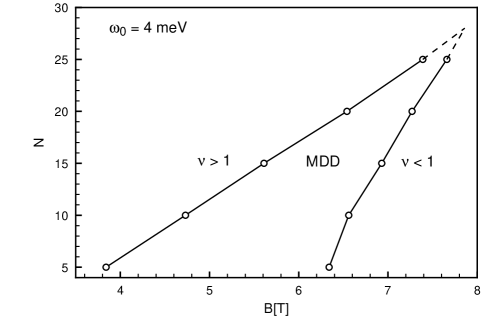
FIG. 2.: B-N phase diagram of the MDD for $\omega_{0}=4{\rm eV}$ obtained solving the Kohn-Sham equations as in Ref. [10].

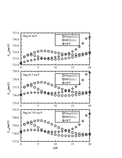
FIG. 3.: Evolution of the energy for the MDD and the “one-hole” states as a function of the magnetic field for a 20 electron quantum dot. $\omega_{0}=3meV.$

REFERENCES

- [1] T. Chakraborty, Comm. on Cond. Matt. Phys. 16, 35 (1992).
- [2] R. Ashoori, Nature, 379, 413 (1996).
- [3] The Quantum Hall effect, edited by R. E. Prange and S. M. Girvin, (Springer-Verlag, New York, 1990).
- [4] The quantum Hall effects: integral and fractional, by T. Chakraborty and P. Pietiläinen, (Springer-Verlag, New York, 1995).
- [5] A. H. MacDonald, S. R. Eric Yang, and M. D. Johnson, Aust. J. Phys. 46, 345 (1993).
- [6] C. de Chamon and X.-G. Wen, Phys. Rev. B 49, 8227 (1994).
- [7] Kang-Hun Ahn, J. H. Ohn, and K. J. Chang, Phys. Rev. B 52, 13757 (1995).
- [8] O. Klein, C. de Chamon, D. Tang, D. M. Abusch-Magder, U. Meirav, X.-G. Wen, and M. Kastner, Phys. Rev. Lett. 74, 785 (1995).
- [9] O. Klein, D. Goldhaber-Gordon, C. de Chamon, and M. A. Kastner, Phys. Rev. B 53, R4221 (1996).
- [10] M. Ferconi and G. Vignale, Phys. Rev. B 50, 14722 (1994).
- [11] T. H. Stoof and Gerri E. W. Bauer, Phys. Rev. B 52, 12143 (1995).
- [12] O. Heinonen, M. I. Lubin, and M. D. Johnson, Phys. Rev. Lett. 75, 4110 (1995).
- [13] M. Ferconi, M. R. Geller, and G. Vignale, Phys. Rev. B 52, 16357 (1995).
- [14] Handbook of Mathematical Functions, Ed. by M. Abramowitz and I. A. Stegun, (Dover Publications, Inc., New York, 1970).
- [15] The Bateman Manuscript Project, Higher Transcendental functions, vol. 1, Eds. A. Erdély, W. Magnus, F. Oberhettinger, and F. G. Tricomi, (McGraw-Hill, New York, Toronto, London, 1953).
- [16] J. H. Oaknin, L. Martín-Moreno, J. J. Palacios, and C. Tejedor, Phys. Rev. Lett. 74, 5120 (1995).