Casimir Forces at Tricritical Points:
Theory and Possible Experiments

Abstract

Using field-theoretical methods and exploiting conformal invariance, we study Casimir forces at tricritical points exerted by long-range fluctuations of the order-parameter field. Special attention is paid to the situation where the symmetry is broken by the boundary conditions (extraordinary transition). Besides the parallel-plate configuration, we also discuss the geometries of two separate spheres and a single sphere near a planar wall, which may serve as a model for colloidal particles immersed in a fluid. In the concrete case of ternary mixtures a quantitative comparison with critical Casimir and van der Waals forces shows that, especially with symmetry-breaking boundaries, the tricritical Casimir force is considerably stronger than the critical one and dominates also the competing van der Waals force. Therefore the prospects for an experimental verification of the Casimir effect at tricritical points should be good.

1 Introduction

In 1948 it was discovered by Casimir [1] that vacuum fluctuations of the electromagnetic field give rise to an attractive force between uncharged conducting capacitor plates. Qualitatively speaking, the reason for the Casimir effect is that the plates impose boundary conditions on the zero-point fluctuations of the electromagnetic field and, as a consequence, the vacuum energy of the system is changed in a distance-dependent way. Due to the masslessness of photons, the resulting interaction, the Casimir force, is long-ranged. In a recent experiment by Lamoreaux [2] the original result of Casimir was verified to within $5\%$ accuracy.

In the context of statistical and condensed matter physics it was pointed out by Fisher and de Gennes [3] that an analogous effect should also exist at or near a critical point when the system considered is restricted by boundaries. In this case the critical (long-range) fluctuations of the order-parameter field play the role of vacuum fluctuations and the critical theory, in a continuum description, is formally equivalent to a massless quantum field theory.

In recent years the Casimir effect in statistical physics was studied theoretically by conformal and perturbative methods [4, 5, 6, 7, 8, 9, 10, 11, 12, 13, 14] and by means of Monte Carlo simulations[15]. However, so far a direct experimental verification of the statistical Casimir effect has not been accomplished. For a review we refer to the book by Krech [16]. Most of the theoretical efforts concentrated on the parallel-plate (PP) geometry and on ordinary critical points. Consider for example a fluid that is confined between two planar walls, with the lateral extension $M$ and the area $A\propto M^{2}$, in a distance $D$ from each other. Further, we assume that $M\gg D$. In this system the singular part of the free energy at the bulk critical point $T_{c}$ asymptotically takes the form [11, 16]

$$\frac{F_{S}}{A\,k_{B}T_{c}}\approx Mf_{\mbox{\tiny bulk}}+f_{a}+f_{b}+\delta f_{ab}\,,$$ (1)

where $k_{B}$ denotes the Boltzmann constant, $f_{\mbox{\tiny bulk}}$ is the bulk contribution, and $f_{a}$ and $f_{b}$ are the surface free energies of surface $a$ and $b$, respectively. The last term (1) is the Casimir energy. As a consequence of the scaling invariance of $F_{S}$ it can be written as

$$\delta f_{ab}=\Delta_{ab}\,D^{-(d-1)}\>.$$ (2)

It is the contribution to the free energy that takes into account the interaction between the walls due to long-range fluctuations. The amplitude $\Delta_{ab}$ in (2) is a universal quantity below the upper critical dimension $d^{*}$ and only depends upon the surface universality classes to which the walls belong. For a detailed analysis of the scaling behavior of $F_{S}$ away from bulk criticality we again refer to Refs. [11, 16].

How do surfaces affect critical fluctuations? Now, in the framework of continuum field theory as for example the $n$-vector model, the surface influence can be modeled by additional fields like the surface magnetic field $h_{1}$ and a local temperature perturbation (surface enhancement), taking into account the interaction with an adjacent noncritical medium and a changed coupling strength near the surface within the medium, respectively[17]. At $T_{c}$, where the bulk value of the order parameter—let us call it $\Phi$—is zero, the tendency to order near the surface can be reduced (ordinary transition), increased (extraordinary transition), or, as a third possibility, the surface can be critical as well (special transition). In the case of both the ordinary and the special transition the symmetry with respect to $\Phi\to-\Phi$ at the surface is unbroken. In opposition to that, at the extraordinary transition the symmetry is broken explicitly or spontaneously [18]. In this case the surface is in an ordered state, but the bulk, far away from the boundary, is disordered, the local magnetization $m(z)$ decaying as $\sim z^{-\beta/\nu}$ for macroscopic distances [17].

In the present work, we focus our attention on systems at a tricritical point, in particular on those with symmetry-breaking boundaries. While the existing work on the tricritical Casimir effect concentrated on symmetry-preserving surfaces [11, 16], there are several reasons why also the “extraordinary” situation at tricritical points should be considered. It is known that for symmetry-preserving boundary conditions the tricritical Casimir amplitude is considerably larger than the corresponding critical amplitude [11, 16]. The same tendency can be expected for symmetry-breaking boundaries. Additionally, the best candidates for the experimental verification of the Casimir effect at tricritical points, ternary fluid mixtures, in general lead to a model with symmetry-breaking boundary conditions. Consider for instance a ternary mixture near its tricritical point. The order parameter $\Phi$ of this system is a linear combination of concentrations of the individual chemical components[19]. A surface—for example a container wall or the surface of a colloid particle immersed in the fluid—will generically favor one of the chemical components, which means that the $\Phi\rightarrow-\Phi$ symmetry is broken explicitly by the surface. In turn, in the framework of lattice or continuum models this is taken into account by a nonzero surface field $h_{1}$. Since $h_{1}$ is relevant in the sense of the renormalization group this leads to the scenario of the extraordinary transition [17, 18]. The case of ³He-⁴He mixtures, more subtle than the one of ternary mixtures, will be addressed in Sec. 5.

Motivated by an experiment by Ducker et al. [21], where the van der Waals force between a spherical (mesoscopic) particle and a container wall was measured, we also consider (besides the PP geometry) various spherical geometries. Recently, it was pointed out [24, 13, 14] that configurations like two spheres immersed in a critical fluid and a single sphere near a planar wall can be conformally mapped to two concentric spheres. Further, due to the rotational symmetry the latter can be treated on the MF level[24], and, employing the conformal invariance of $F_{S}$, the Casimir force can be calculated in the former configurations as well [13, 14].

The rest of this article is organized as follows: In Sec. 2 and 3 the tricritical Casimir forces are calculated for planar and spherical geometries, respectively In Sec. 4 a quantitative comparison between van der Waals forces and Casimir forces with symmetry-breaking boundaries is carried out. In Sec. 5 possible experiments, especially on ternary or quaternary mixtures, are discussed, and the issue of ³He-⁴He mixtures is addressed.

2 Parallel-Plate Geometry

We first derive the Casimir forces in the geometry of parallel plates. Since $d=3$, the spatial dimension we are interested in, is the upper critical dimension $d^{*}$ for tricritical phenomena, we have to solve the model on the MF level and subsequently improve the result by renormalization-group considerations [20]. Our starting point is the Landau-Ginzburg functional for an $n$-component order parameter at the tricritical point

$${\cal H}=\int_{V}\,d^{3}r\,{\cal L}$$ (3)

with

$${\cal L}=\frac{1}{2}({\bf\nabla}\vec{\Phi})\cdot({\bf\nabla}\vec{\Phi})+\frac{g}{6!}\left(\vec{\Phi}^{2}\right)^{3}\>,$$ (4)

where $V$ denotes that the integration ranges over the whole critical medium. The Casimir force in the PP geometry can be written as [16]

$$\frac{1}{A}\frac{dF_{s}}{dD}=-k_{B}T_{c}\,\langle{\cal T}_{zz}\rangle\>,$$ (5)

where $A$ denotes the area of the plates that, as said above, are assumed to have a linear extension $M$ much larger than the vertical distance $D$. In Eq. (5) and in the following $T_{c}$ denotes both critical and tricritical temperatures. Further, the cartesian stress tensor ${\cal T}_{ij}$ is given by [26]

$${\cal T}_{ij}=\partial_{i}\vec{\Phi}\cdot\partial_{j}\vec{\Phi}-\delta_{ij}{\cal L}-\frac{1}{4}\frac{d-2}{d-1}\left(\partial_{i}\partial_{j}-\delta_{ij}\nabla^{2}\right)\vec{\Phi}^{2}\>,$$ (6)

and with (1), (2), and (5) one obtains the relation[16]

$$\Delta_{ab}=\frac{D^{d}}{d-1}\,\langle{\cal T}_{zz}\rangle\>$$ (7)

between the Casimir amplitude introduced in (2) and the $zz$ component of the stress tensor.

To derive the MF equation from ${\cal H}$, we let $\vec{\Phi}$ point in the $1$-direction of the $n$-dimensional order-parameter space. Introducing the rescaled field $\sigma=(g/5!)^{1/4}\Phi_{1}$, the MF equation reads

$$\frac{d^{2}\sigma}{dz^{2}}-\sigma^{5}=0\>,$$ (8)

and, after multiplication by $d\sigma/dz$, the first integral of this equation is found to be

$$I_{\mbox{\tiny PP}}=\left(\frac{d\sigma}{dz}\right)^{2}-\frac{1}{3}\,\sigma^{6}\>.$$ (9)

It only depends on the distance $D$ between the plates and on the boundary conditions. The latter can be implemented a posteriori by selecting solutions that, in the case of symmetry-breaking surfaces, become singular upon approaching the boundaries $z=\pm D/2$. In the following we only consider the situation where $\sigma(z)$ tends to $+\infty$ at both plates and, due to the symmetry, has a minimum at $z=0$. We denote this situation as $\uparrow\uparrow$ boundary conditions, as opposed to the situation where for instance $\sigma$ tends to $\infty$ at one surface and to $-\infty$ at the other, denoted as the $\uparrow\downarrow$ case. With the same boundary conditions at both surfaces the resulting Casimir force is generally attractive. In the other case, for example with $\uparrow\downarrow$ boundary conditions, it is repulsive [16]. This also holds for the spherical geometries to be discussed in Sec. 3.

It is straighforward to show from (8) that the first integral is given by

$$I_{\mbox{\tiny PP}}=-8\sqrt{3}\,\left(\frac{c_{6}}{D}\right)^{3}$$ (10)

with the constant

$$c_{6}=\int_{1}^{\infty}\frac{dx}{\sqrt{x^{6}-1}}=0.70109\ldots\>.$$ (11)

Next, there is a close relationship between $I_{\mbox{\tiny PP}}$ and the $zz$-component of the stress tensor (6) that reads [14]

$${\cal T}_{zz}=\left(\frac{30}{g}\right)^{1/2}I_{\mbox{\tiny PP}}\>.$$ (12)

and can be verified from (6) and (9). Eventually, the MF (or zero-loop) result for the tricritical Casimir amplitude is

$$\Delta_{\uparrow\uparrow}=-\frac{13.0768...}{g^{1/2}}\>.$$ (13)

The analogous result for a critical point was derived in Ref. [10].

The Casimir amplitude in (13) as it stands still depends on the arbitrary coupling constant $g$. In order to remove this dependence, we have to invoke standard renormalization-group arguments. In the scaling limit, the singular part of the free energy (1) should take the form

$${F_{S}}(M,D,g)=k_{B}T_{c}\>{\cal F}(M/D,\bar{g}(l)),$$ (14)

where $l\ll 1$ is the spatial rescaling factor and the running coupling constant $\bar{g}(l)$ is given by [28]

$$\bar{g}(l)=\frac{240\,\pi^{2}}{(3n+22)\,|\mbox{ln}l|}\,\>.$$ (15)

Other fields (like $\tau$, $h_{1}$, etc.) that are not listed in the argument on the left-hand side of (14) are assumed to be adjusted to their fixed-point values and, thus, are unaffected by the rescaling.

In $d=3-\epsilon$ dimensions the MF amplitude (13) would yield the leading contribution in a perturbative series, in which (after the subtraction of uv divergences) the renormalized coupling constant could be set to its $l\to 0$ value $g^{*}\propto\epsilon$. For $d=d^{*}$, on the other hand, the coupling must not be set to its fixed-point value $g^{*}=0$ in (13). Instead, the rescaling parameter $l$ can be replaced by $a/D$ [37], where $a$ is a microscopic length scale, typically in the range of a few Å, as opposed to $D$ which we assume to be mesoscopic or macroscopic, of the order of $\mu$m, say.

With (5) and (13) and after it has been brought into the scaling form with (14), the result for the Casimir force reads

$$\frac{f^{tc}_{\mbox{\tiny PP}}}{A}\simeq-0.54\,k_{B}T_{c}\,\left(3n+22\right)^{1/2}\left(\mbox{ln}\,D/a\right)^{1/2}D^{-3}\>.$$ (16)

Corrections to (16) from higher-order terms in the perturbative series are suppressed logarithmically, i.e., by powers of $\mbox{ln}\,D/a$.

At the first glance it appears that the logarithmic term in (16) modifies the $D$-dependence of the Casimir force from $\sim D^{-3}$ to $\sim(\mbox{ln}\,D)^{1/2}|\,D^{-3}$. That this modification can also be regarded as a correction and, thus, may be dropped when one only considers the leading asymptotic behavior, can be seen by rewriting $\mbox{ln}\,D/a=\mbox{ln}\,D_{0}/a+\mbox{ln}\,D/D_{0}$, where $D_{0}$ is another macroscopic constant length scale. Then the result for the Casimir amplitude is

$$\Delta_{\uparrow\uparrow}^{tc}=-0.27\,(3n+22)^{1/2}\,\Omega_{0}\,,$$ (17)

where $\Omega_{0}$ is defined as

$$\Omega_{0}:=\left(\mbox{ln}\,\frac{D_{0}}{a}\right)^{1/2}\>.$$ (18)

As opposed to the situation below $d^{*}$, where one really finds a universal scalar amplitude, at a tricritical point in $d=d^{*}=3$ we have additionally a nonuniversal scalar factor $\Omega_{0}$, expressing a dependence of the physics at a macroscopic scale $D_{0}$ on the macroscopic scale $a$. This phenomenon does not occur in a tricritical system with both surfaces preserving the symmetry [11]. Then the leading asymptotic contribution to the Casimir energy is given by the universal amplitude of the Gaussian model ($g=0$ in the Eq. (4)). In this case only corrections to scaling depend on the microscopic scale. A situation largely analogous to the symmetry-breaking case discussed above is known from polymers near the $\theta$-point [22].

Even if we do not know $D_{0}/a$ in (18) in practice, the dependence on this ratio, as it comes in as the square root of the logarithm, turns out to be very weak. For instance when $D_{0}/a$ is varied over two orders of magnitude from 100 to 10000 (which should be a reasonable range from the point of view of the experiments), $\Omega_{0}$ varies between 2.1 and 3, i.e., it changes only by about 40$\%$.

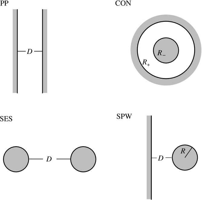
Figure 1: The geometries of parallel plates (PP), concentric spheres (CON), spheres of equal size (SES), and sphere and planar wall (SPW) considered in Sec. 2 and 3. The gray areas represent the noncritical medium (wall).

3 Spherical Geometries

Following Ref. [14] the conformal invariance at a critical point can be exploited to calculate Casimir forces in conformally equivalent geometries. For instance in the highly symmetric geometry of two concentric spheres (CON) with radii $R_{-}$ and $R_{+}$ of Fig. 1, the singular part of the free energy only depends upon $\rho=R_{-}/R_{+}$. The derivative of $F_{S}$ with respect to $\rho$ is given by [14]

$$\rho\;\frac{\rm d}{{\rm d}\rho}\,F_{S}(\rho)=k_{B}T_{c}\>S_{d}\;r_{0}^{d}\>\langle{\cal T}_{rr}(r_{0})\rangle_{\mbox{\tiny CON}}\>,$$ (19)

where ${\cal T}_{rr}$ is the projection of the stress tensor (6) on the radial direction, $S_{d}$ denotes the surface area of the $d$-dimensional unit sphere, and $r_{0}$ is an inner point between the two spheres.

The MF equation for the rescaled order-parameter field $\sigma$ that now only depends on $r$ takes the form

$$\frac{d^{2}\sigma}{dr^{2}}+\frac{d-1}{r}\frac{d\sigma}{dr}-\sigma^{5}=0.$$ (20)

This equation is a differential equation of the Emden-Fowler type [29, 24, 14], and a first integral exists (only) in $d=3$:

$$I_{\mbox{\tiny CON}}=r^{3}\frac{d^{2}\sigma}{dr^{2}}+r^{2}\sigma\frac{d\sigma}{dr}-\frac{1}{3}r^{3}\sigma^{6}\>.$$ (21)

Like in the PP case we are interested in $\uparrow\uparrow$ boundary conditions, i.e. where $\sigma$ becomes infinite at both the inner and the outer sphere, respectively. In this case there exists a relation between $\rho$ and $I_{\mbox{\tiny CON}}$ that can be expressed in the form

$$\rho=\exp\left[-\sqrt{\frac{3}{pq}}\,F(\alpha,k)\right]\>,$$ (22)

where $F(\alpha,k)$ is the elliptic integral of the first kind [32], and the arguments are

$$\alpha = 2\,\mbox{arctan}\left(\sqrt{\frac{q}{p}}\,\right)$$

$$k = \sqrt{\frac{(p+q)^{2}-a^{2}}{4pq}}$$ (23)

with

$$p = \sqrt{b^{2}+\frac{9}{4}a^{2}}$$

$$q = \sqrt{b^{2}+\frac{1}{4}a^{2}}$$

$$a = A_{+}+A_{-}$$

$$b = \frac{\sqrt{3}}{2}\left(A_{+}-A_{-}\right),$$ (24)

and the dependence of $A_{\pm}$ on $I_{\mbox{\tiny CON}}$ is given by

$$A_{\pm}=\left(-\frac{3}{2}I_{\mbox{\tiny CON}}\pm\frac{1}{8}\sqrt{1+144I_{\mbox{\tiny CON}}^{2}}\right)^{1/3}\>.$$ (25)

Moreover, analogously to (12) the relation between the first integral and the stress tensor reads

$$r_{0}^{3}\,T_{rr}(r_{0})=\left(\frac{30}{g}\right)^{1/2}\!I_{\mbox{\tiny CON}}\>$$ (26)

such that on the MF level the Casimir force in (19) can be obtained as a function of $\rho$.

Now, the concentric geometry is conformally equivalent to various other geometries [14]. For example by inversion at an inner point in between the concentric spheres the system is mapped to a geometry where two separate spheres are immersed in a surrounding (critical) medium. If the point of inversion lies at the geometric mean $(R_{-}\,R_{+})^{1/2}$, one obtains spheres of equal size (SES). Likewise, inversion at one of the radii, $R_{-}$ or $R_{+}$, generates a geometry in which a single sphere is placed in a given distance from a planar wall (SPW). All the geometries treated in the present work are depicted in Fig. 1.

At (and above) the upper critical dimension conformal invariance does not hold anymore [23]. However, on the MF level the field theory described by (4) is conformally invariant just in $d=3$. Further, since we are only interested in boundary conditions that correspond to renormalization-group fixed points, conformal invariance is not affected by the boundaries either[31]. Hence, the MF approximation to the Casimir force, obtained for instance in the CON geometry, can directly be translated to other conformally equivalent geometries (like SPW or SES).

As discussed in more detail in Ref. [14], $F_{S}$ depends upon certain invariant cross ratios of the geometric dimensions [23], a convenient parameter to quantify the dependence on the geometry being

$$\kappa=\left\{\begin{array}[]{ll}\frac{1}{2}\left(\rho+{1/\rho}\right)&\quad\mbox{for CON}\\[5.69054pt] D^{2}/(2R^{2})+2D/R+1&\quad\mbox{for SES}\\[5.69054pt] D/R+1&\quad\mbox{for SPW}\end{array}\right.\>.$$ (27)

Thus for instance the force in the SPW geometry derived from the known result of the CON geometry, is given by

$$f^{tc}_{\mbox{\tiny SPW}}=-\frac{dF_{S}}{dD}=-\frac{dF_{S}}{d\rho}\frac{d\rho}{dD}\>,$$ (28)

where the first factor on the right-hand side can be derived from (19), and $d\rho/dD$ can be calculated from (27). With (26) we obtain the MF result

$$f^{tc}_{\mbox{\tiny SPW}}=\,k_{B}T_{c}\,\left(\frac{30}{g}\right)^{1/2}\frac{I_{\mbox{\tiny CON}}(\rho)}{(D^{2}+2DR)^{1/2}}\>.$$ (29)

As the next step, in the new geometry, the MF result has to be improved by means of scaling arguments, much in the same way as discussed in Sec. 2 for the PP geometry. The renormalization-group improvement again yields a nonuniversal factor $\Omega_{0}$ (see Eq. (18)), where now distance scales of the new geometry (SPW or SES) enter.

Eventually, the results for the Casimir force in the SPW and SES geometries are given by

$$f^{tc}_{\mbox{\tiny SPW}}=k_{B}T_{c}(6n+44)^{1/2}\,\Omega_{0}\,\frac{I_{\mbox{\tiny CON}}(\rho)}{(D^{2}+2DR)^{1/2}}\>$$ (30)

and

$$f^{tc}_{\mbox{\tiny SES}}=k_{B}T_{c}(6n+44)^{1/2}\,\Omega_{0}\,\frac{2\,I_{\mbox{\tiny CON}}(\rho)}{(D^{2}+4DR)^{1/2}}\>,$$ (31)

respectively, where $\rho=\rho(D)$ can be obtained from (27). For the concrete example of a ternary mixture with $T_{c}=300\,$K, spheres with a radius $R=1\,\mu$m, and with the nonuniversal factor set to$\Omega_{0}=2$, the results are plotted in Figs. 1 and 2 and compared with the van der Waals forces.

4 Comparison with the critical Casimir effect and van-der-Waals forces

For a quantitative comparison between the tricritical and the critical Casimir effect and the van der Waals forces let us first consider the PP geometry and a system with an Ising-like order parameter ($n=1$). Then from (17) we find for the tricritical Casimir amplitude $\Delta_{\uparrow\uparrow}^{tc}=-1.35\,\Omega_{0}$, where the nonuniversal factor $\Omega_{0}$ was defined in (18).

In a recent preprint [30], Krech obtained $\Delta_{\uparrow\uparrow}^{c}\simeq-0.35$ for the Casimir amplitude of a critical Ising-like system in $d=3$. Hence, taking into account that $\Omega_{0}\,\vbox{\hbox{$\buildrel\textstyle>\over{\sim}$}}2$, the tricritical Casimir amplitude is about seven times larger then the corresponding critical amplitude, and, at least as far as the magnitude of the force is concerned, tricritical points should be better suited for the experimental verification of the Casimir effect than critical points at comparable temperatures.

How does the Casimir effect compare with the van der Waals force? The result for the van der Waals force in the PP geometry is given by [33]

$$\frac{f_{\mbox{\tiny PP}}^{vdW}}{A}=-\frac{H}{6\pi}\,\frac{1}{D^{3}}\>$$ (32)

where $H$ is the Hamaker constant, a material-dependent quantity that in most systems lies somewhere between $10^{-19}$J and $10^{-21}$J [33]. For the sake of concreteness, let us set the Hamaker constant to a typical value of about $H=10^{-20}$J. Taking then the ratio between tricritical Casimir and van der Waals force we find

$$\frac{f_{\mbox{\tiny PP}}^{tc}}{f_{\mbox{\tiny PP}}^{vdW}}\simeq 0.07\,\Omega_{0}\,T_{c}/\mbox{K}\>.$$ (33)

Hence, even if the tricritical temperature were about $1\,$K—in Helium mixtures it is $0.867\,$K— and we set $\Omega_{0}\simeq 2$ as before, the Casimir force amounts to more than $10\%$ of the van der Waals force. This is different if symmetry-preserving boundaries are considered; in this case the Casimir force is merely a $1\%$ effect [11]. For ternary mixtures, where usually systems are studied with $T_{c}$ near room temperature, the Casimir force becomes even considerably stronger than the van der Waals attraction.

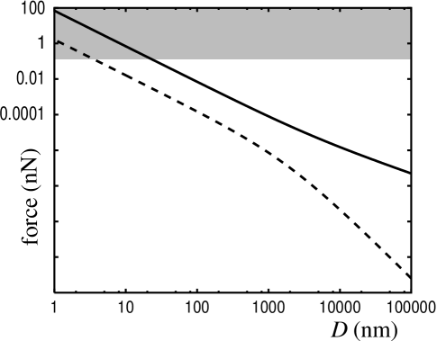
Figure 2: The tricritical Casimir force (solid) and the van der Waals force (dashed) in SPW geometry of Fig. 1 for $T_{c}=300\,$K, particle radius $R=1\,\mu$m and Hamaker constant $H=10^{-20}\,$J. The grey shaded area indicates the regime with force $f\,\vbox{\hbox{$\buildrel\textstyle>\over{\sim}$}}0.2\,$nN where direct measurements should be feasible (cf. Ref. [20].)

As the next example let us consider the case SPW in Fig. 1. In this geometry direct measurements of the van der Walls force by means of an atomic force microscope were reported by Ducker et al. [21], and it should be feasible to carry out a similar measurement with a critical or tricritical fluid. For the SPW geometry an approximative expression for the nonretarded van der Waals force [33]

$$f_{\mbox{\tiny SPW}}^{vdW}=-\frac{2H}{3}\,\frac{R^{3}}{(D+2R)^{2}D^{2}}$$ (34)

can be obtained. A direct comparison between (34) and our result (30) is carried out in Fig. 2. Again, $H$ was set to the typical value of $10^{-20}$ J. For the Casimir force (solid curve) we assumed that $T_{c}=300\,$K and $\Omega_{0}=2$. For large distances $D\gg R$, the Casimir force decays more slowly than the van der Waals result (dashed line), the former behaving as $\sim D^{-3/2}$ and the latter as $D^{-4}$. For small (but still macroscopic) distances distances $a\ll D\ll R$, both the Casimir and the van der Waals force show the same $D$-dependence $\sim D^{-2}$. The reason for this coincidence is that this limit is closely connected to the PP geometry[14], the ratio of amplitudes being given by (33). The grey shaded area in Fig. 2 shows the regime with forces $\,\vbox{\hbox{$\buildrel\textstyle>\over{\sim}$}}0.2\,$nN, where the measurement with an atomic force microscope, like the one reported in Ref. [21], should be possible.

Figure 3: The tricrittical Casimir force (solid) and the asymptotic van der Waals results (dashed) in SES geometry of Fig. 1 with the same parameters as in Fig. 2.

Eventually, the results for the SES geometry are displayed in Fig. 3. For the nonretarded van der Waals force the two asymptotic power laws for small and large distances (dashed lines) are taken from Ref. [33]. The solid line shows the result of Eq. (31), again for $T_{c}=300\,$K, $\Omega_{0}=2$, and $R=1\,\mu$m. For $D\gg R$ the curves approach zero as $\sim D^{-6}$ (van der Waals) and $\sim D^{-2}$ (Casimir), respectively. Again, in both cases the force behaves as $\sim D^{-2}$ for short distances. In particular, this means that $f_{\mbox{\tiny SES}}^{tc}$ has the same $D$-dependence in both limits for $D\ll R$ and $D\gg R$, with different amplitudes, however, as indicated by the swerve in Fig. 3 at the crossover distance $D\simeq R=1\,\mu$m.

5 Prospects for Experiments

Probably the best candidates for experiments on the tricritical Casimir effect are ternary or quaternary mixtures of fluids, the latter with the advantage that they can be “tuned” to have a tricritical point at atmospheric pressure [38]. The order parameter $\Phi$ in these systems is Ising-like, a linear combination of concentrations of the single components. As said in the Introduction, the surface will generically favor one of the components of the fluid, amounting to an explicit symmetry breaking at the surface. In the scaling limit this leads to the scenario of the extraordinary transition[17, 18]. Additionally, systems can be chosen with their $T_{c}$ at or around the room temperature. Hence, as the singular part of the free energy behaves as $\sim T$, the magnitude of the Casimir force in fluid mixtures should be larger by about two orders of magnitude than in Helium mixtures (to be discussed in the next paragraph).

In mixtures of ³He and ⁴He the tricritical point is located at $T_{c}=867$mK and $x_{c}=0.675$ mole fraction of ³He. It is well known that pure ⁴He belongs to the universality class of the ordinary transition, because the quantum-mechanical wave function that describes the superfluid state goes to zero at the surface. Now, as long as the fraction of ³He is not too large ($x\,\vbox{\hbox{$\buildrel\textstyle<\over{\sim}$}}0.54$) also in He mixtures the scenario of the ordinary transition holds [34]. However, for $x$ beyond a certain value $x_{s}\simeq 0.54$ a superfluid layer (rich in ⁴He) forms already above the $\lambda$ line [34], i.e., in the language of surface critical phenomena a surface transition [17] takes place. Since the superfluid layer is effectively two-dimensional and the system possesses a continuous $O(2)$ symmetry, it is in a Kosterlitz-Thouless phase [35]. The latter was also verified by the experiment [36]. Note that there is no physical $h_{1}$ in this system that couples to the order parameter. In the framework of the continuum description the surface transition is triggered by the negative surface enhancement [25].

Upon approaching the $\lambda$-line from above in the concentration range $x_{s}<x\leq x_{c}$, due to the growing correlation length the superfluid layer becomes thick and a dimensional crossover [39] from the Kosterlitz-Thouless phase to a three-dimensional superfluid phase should take place [40]. As a consequence, Helium mixtures in the mentioned concentration range also appear to be a candidate for a system with symmetry-breaking boundary conditions. However, since the dimensional crossover, in particular the one between a Kosterlitz-Thouless phase (in $d=2$) and the ordered phase of the $XY$-model (in $d=3$), is not fully understood, it is far from clear that the scenario of the extraordinary transition applies [34]. However, concerning the Casimir force and other critical surface effects there should definitely be a difference between $x<x_{s}$ and $x>x_{s}$, presumably with a qualitatively new type of Casimir amplitude for $x>x_{s}$ that can not be adequately described in the framework of the known surface universality classes (ordinary, extraordinary, or special).

An interesting question that could also be addressed in such experiments is related to critical dynamics. The results for the Casimir force presented in the previous sections are ensemble averages. Due to fluctuations in space and time, individual members of an ensemble deviate from the thermal average, i.e., for instance in the PP geometry the local pressure will vary in lateral direction. Also the van der Waals force, being closely related to the original electromagnetic Casimir effect, is an average over fluctuations, this time of quantum-mechanical nature, however. The typical time scale on which fluctuations of the van der Waals force take place is given by $D/c$, where $c$ is the speed of light. On a presumably much larger time scale, behaving as $\sim D^{\zeta}$, the fluctuations of the Casimir force take place, where $\zeta$ denotes the dynamic (equilibrium) exponent of model H in the terminology of Ref. [41]. In the PP geometry when $M\gg\xi\gg D$ this time dependence would be probably absent because the average over the lateral directions is taken. In the SPW geometry, however, the time dependence of the critical fluctuations taking place on a potentially macroscopic scale should be observable.

Finally we should like to emphasize the long-range nature of the Casimir forces specific to symmetry-breaking boundary conditions. For the critical case it was pointed out by de Gennes [42] and studied in more detail in Refs. [13, 14] that in the SES geometry for large distances the Casimir free energy decays as $\sim D^{-2\beta/\nu}$. With $\beta/\nu\simeq 0.52$ for the $d=3$ Ising system, this is already very close to a Coulomb potential. The tricritical Casimir free energy falls off exactly as $\sim D^{-1}$. As already discussed in Ref. [14], this should have consequences for the thermodynamics of charged stabilized colloids when the correlation length in the solvent becomes comparable or larger than the average distance of colloid particles. In particular we expect reversible flocculation near a critical or tricritical point. Flocculation phenomena in fluid mixtures near critical points have already been reported in the literature[43, 45].

6 Summary and Concluding Remarks

We studied the Casimir effect at tricritical points with symmetry-breaking boundary conditions. The case of symmetry-preserving boundaries was treated earlier in the literature by Krech and Dietrich [11]. The leading asymptotic behavior of the Casimir force in $d=3$ is determined by the mean-field theory, improved by renormalization-group considerations. Different from critical systems and tricritical systems with symmetry-preserving boundaries, where the Casimir amplitude is universal, at a tricritical point with symmetry-breaking boundaries a nonuniversal factor occurs. As expressed in (18), this factor depends on the ratio between a typical macroscopic and a microscopic length, and we estimated it to lie between 2 and 3 for a typical experimental setting.

Our calculations were restricted to bulk tricriticality, but the results derived should hold more generally when the correlation length $\xi$ is larger or much larger than $D$. In case that $\xi$ becomes comparable to $D$, the force should decrease, and in particular for $\xi\ll D$ it should decay exponentially.

Up to date neither the critical nor the tricritical Casimir effect have been verified in the experiment. The most promising candidates for experiments on the tricritical Casimir effect are ternary mixtures and quaternary mixtures of fluids. Concerning the geometry we suggested either the parallel-plate geometry, in which the electromagnetic Casimir effect was verified successfully [2], or the geometry of a sphere near a planar wall, in which the van der Waals force was measured with an atomic force microscope [21]. In particular in fluid mixtures the tricritical Casimir effect should dominate the van der Waals force.

As another candidate for experiments on the tricritical Casimir effect we discussed Helium mixtures. In this case it turned out that above a certain concentration $x_{s}>0.54$ and in particular at the tricritical value $x_{c}=0.675$ the surface effects are neither covered by the scenario of the ordinary transition nor by the one of the extraordinary transition, for the surface undergoes a transition to a Kosterlitz-Thouless phase [34]. Hence, it requires further theoretical studies to obtain the corresponding Casimir amplitudes.

Finally we mention that there are other obvious directions in which the theoretical work on the statistical Casimir effect should be extended. Besides critical and tricritical points, complex fluid mixtures exhibit a variety of interesting critical phenomena, like for example double or quadruple critical points, discussed in the literature under the heading of reentrant phase transitions [44]. The parameters in these systems, the temperature, the pressure, and the various concentrations can be well controlled, and the experiments reveal an intriguing spectrum of phenomena as for example the doubling of critical exponents at a double critical point [45]. It would be certainly of interest to study surface critical phenomena and, especially, the Casimir effect also at these special critical points.
Acknowledgements: We thank H. W. Diehl for a helpful discussion in the early stage of this work and especially E. Eisenriegler for the critical reading of the manuscript, helpful comments, and hints to the literature. This work was supported in part by the Deutsche Forschungsgemeinschaft through Sonderforschungsbereich 237.

References

- [1] H. B. G. Casimir, Proc. K. Ned. Akad. Wet. 51, 793 (1948); for a recent review on the Casimir effect in QED, see G. Plunien, B. Müller, and W. Greiner, Phys. Rep. 134 (1986) 87.
- [2] S. Lamoreaux, Phys. Rev. Lett. 78 (1997) 5.
- [3] M. E. Fisher and P.-G. de Gennes, C. R. Acad. Sci. Ser. B 287 (1978) 207.
- [4] H. W. J. Blöte, J. L. Cardy, and M. P. Nightingale, Phys. Rev. Lett. 56 (1986) 742.
- [5] I. Affleck, Phys. Rev. Lett. 56 (1986) 746.
- [6] J. L. Cardy, Nucl. Phys. B 275 (1986) 200.
- [7] T. W. Burkhardt and T. Xue, Phys. Rev. Lett. 66 (1991) 895; Nucl. Phys. B345 (1991) 653.
- [8] T. W. Burkhardt and E. Eisenriegler, Nucl. Phys. B 424 [FS] (1994) 487.
- [9] K. Symanzik, Nucl. Phys. B190, [FS3] (1981) 1.
- [10] M. P. Nightingale and J. O. Indekeu, Phys. Rev. Lett. 54 (1985) 1824; J. O. Indekeu, M. P. Nightingale, and W. V. Wang, Phys. Rev. B 34 (1986) 330.
- [11] M. Krech and S. Dietrich, Phys. Rev. Lett. 66 (1991) 345; 67 (1991) 1055; Phys. Rev. A 46 (1992) 1886; 46 (1992) 1922.
- [12] E. Eisenriegler and M. Stapper, Phys. Rev. B 50 (1994) 10009.
- [13] T. W. Burkhardt and E. Eisenriegler, Phys. Rev. Lett. 74 (1995) 3189.
- [14] E. Eisenriegler and U. Ritschel, Phys. Rev. B 51 (1995) 13717.
- [15] K. K. Mon, Phys. Rev. Lett. 54 (1985) 2671; M. Krech and D. P. Landau, Phys. Rev. E 53 (1996) 4414.
- [16] M. Krech, The Casimir Effect in Critical Systems (World Scientific, Singapore 1994)
- [17] K. Binder, in Phase Transitions and Critical Phenomena, Vol. 8, C. Domb and J. L. Lebowitz, eds. (London, Academic Press, 1983).
- [18] A. J. Bray and M. A. Moore, J. Phys. A 10 (1977) 1927.
- [19] I. D. Lawrie and S. Sarbach, in Phase Transitions and Critical Phenomena, Vol. 9, C. Domb and J. L. Lebowitz, eds. (London, Academic Press, 1984).
- [20] F. J. Wegner and E. K. Riedel, Phys. Rev. Lett, 7 (1973) 248.
- [21] W. A. Ducker, T. J. Senden, and R. M. Pashley, Nature 353 (1991) 239.
- [22] B. Duplantier, J. Physique (France) 43 (1982) 991.
- [23] J. L. Cardy, in Phase Transitions and Critical Phenomena Vol. 11, Eds. C. Domb and J. L. Lebowitz (Academic Press, London, 1987).
- [24] S. Gnutzmann and U. Ritschel, Z. Phys. B 96 (1995) 391.
- [25] H. W. Diehl, in Phase Transitions and Critical Phenomena Vol 10, Eds. C. Domb and J. L. Lebowitz (Academic Press, London, 1986)
- [26] L. S. Brown, Ann. Phys. (NY) 126 (1980) 135.
- [27] J. Zinn-Justin, Quantum Field Theory and Critical Phenomena, (Clarendon Press, Oxford, 1989).
- [28] E. Eisenriegler and H. W. Diehl, Phys. Rev. D 37 (1988) 5257.
- [29] W. Sarlet and L. J. Bahar, Int. J. Non-Linear Mech. 15 (1980) 133; P. G. Leach, J. Math. Phys. 26 (1985) 2510.
- [30] M. Krech, to be published
- [31] J. L. Cardy, Nucl. Phys. B 240 [FS12] (1984) 514.
- [32] I. S. Gradshteyn and I. M. Ryzhik, Table of Integrals, Series, and Products, (Academic Press, New York, 1980).
- [33] J. N. Israelachvili, Intermolecular and surface forces, (London, Academic Press, 1991).
- [34] S. Leibler and L. Peliti, Phys. Rev. B 29 (1984) 1253; L. Peliti and S. Leibler, J. Physique Lett. 45 (1984) L591.
- [35] J. M. Kosterlitz and D. J. Thouless, J. Phys. C 6 (1973) 1181.
- [36] D. McQueeney, G. Agnolet, and J. D. Reppy, Phys. Rev. Lett. 52 (1984) 1325.
- [37] E. Brezin, J. C. Le Guillou, J. Zinn-Justin, in Phase Transitions and Critical Phenomena Vol 6, Eds. C. Domb and J. L. Lebowitz (Academic Press, London, 1984)
- [38] M. Kahlweit, R. Strey, M. Aratono, M. G. Busse, J. Jen, K. V. Schubert, J. Chem. Phys. 95 (1991) 2842.
- [39] D. J. O’Connor and C. R. Stephens, Phys. Rev. Lett. 72 (1974) 506.
- [40] S. Dietrich, in Phase Transitions and Critical Phenomena Vol 12, Eds. C. Domb and J. L. Lebowitz (Academic Press, London, 1991)
- [41] P. C. Hohenberg and B. I. Halperin, Rev. Mod. Phys. 49 (1977) 435.
- [42] P.-G. de Gennes, C. R. Acad. Sci. Ser. B 292 (1981) 701.
- [43] D. Beysens and S. Leibler, J. Physique. Lett. 43 (1982) L133; D. Beysens and D. Estève, Phys. Rev. Lett. 54 (1985) 2123; D. Beysens, J.-M. Petit, P. Narayanan, A. Kumar, and M. L. Broide, Ber. Bunsen Ges. Phys. Chem. 98 (1994) 382.
- [44] See P. Narayanan and A. Kumar, Phys. Rep. 249 (1994) 135 for an extensive review on this topic.
- [45] A. Kumar, Ind. J. Pure Appl. Phys. 34 (1996) 742.