X-ray edge singularity in integrable lattice models
of correlated electrons

Abstract

We study the singularities in X-ray absorption spectra of one-dimensional Hubbard and $t$–$J$ models. We use Boundary Conformal Field Theory and the Bethe Ansatz solutions of these models with both periodic and open boundary conditions to calculate the exponents describing the power-law decay near the edges of X-ray absorption spectra in the case where the core-hole potential has bound states.

I Introduction

X-ray absorption in a metal can be described by a simple model put forward by Nozières and de Dominicis[1]. An electron from a filled inner shell of one of the nuclei is raised into the conduction band. This generates a local potential $V$ at the position of the nucleus that lost the core-electron, which in turn acts on the (noninteracting) conduction-band electrons and affects the X-ray absorption probability. The situation is described by the Hamiltonian

$$H=\sum_{\vec{k}}\epsilon({\vec{k}})\ c^{\dagger}({\vec{k}})c({\vec{k}})+bb^{\dagger}\sum_{{\vec{k}},{\vec{k}}^{\prime}}V({\vec{k}},{\vec{k}}^{\prime})\ c^{\dagger}({\vec{k}})c({{\vec{k}}^{\prime}})+E_{0}b^{\dagger}b\ ,$$ (1)

where $\epsilon({\vec{k}})$ is the dispersion of the conduction band electrons, $b^{\dagger}$ and $b$ ($c({\vec{k}})$ and $c^{\dagger}({\vec{k}})$) are annihilation and creation operators for the core-hole (for conduction band electrons with wavevector ${\vec{k}}$) and $E_{0}$ is the energy of the core state. As $b^{\dagger}b$ commutes with $H$, the Hilbert space splits into two sectors: in one the core-level is filled ($bb^{\dagger}=0$) and there is no potential whereas in the other one the core level is empty ($bb^{\dagger}=1$) and $V$ acts on the conduction electrons. As was shown in Ref. [1] the inner core disturbance acts as a transient one-body potential on the conduction electrons, which means that one needs to study the response of the conduction band electrons to the potential $V$ applied between times $t=0$ and $t=t^{\prime}$. The X-ray absorption rate can be expressed by the golden rule as

$$I(\omega)\propto\sum_{n}|\langle n|c^{\dagger}_{0}(0)|0\rangle|^{2}\ \delta(\omega+E_{GS}-E_{n}-E_{0})\ ,$$ (2)

where $c_{0}(t)$ annihilates a conduction-band electron at position $\vec{x}=0$ at time $t$, $|0\rangle$ is the ground state at times $t<0$ and $H|0\rangle=E_{GS}|0\rangle$. The r.h.s. of (2) can be expressed in terms of the spectral representation of the Fourier transform of the retarded correlation function $\langle\!\langle b^{\dagger}(t)c_{0}(t)c^{\dagger}_{0}(0)b(0)\rangle\!\rangle$ so that

$$I(\omega)\propto\Im m\int_{0}^{\infty}\ dt\ e^{i\omega t}\langle\!\langle b^{\dagger}(t)c_{0}(t)c^{\dagger}_{0}(0)b(0)\rangle\!\rangle\ .$$ (3)

Near the threshold $\omega_{0}\approx E_{0}$ the intensity $I(\omega)$ displays a characteristic singularity of the form

$$I(\omega)\sim{1\over|\omega-\omega_{0}|^{\alpha}}\ .$$ (4)

For the system (1) the critical exponent $\alpha$ has been determined exactly and is expressed in terms of the phase shift at the Fermi surface [1, 2]. A very interesting case is the one where the local potential $V$ is sufficiently strong to bind a conduction electron [3] (see also Refs. [4, 5]). In this case the absorption spectrum (if $\alpha>0$) features two thresholds with characteristic power-law decays of $I$ as a function of $\omega$ (see Fig. 1a). If $\alpha<0$ there is no discontinuity and $I(\omega)$ goes to zero instead (see Fig. 1b).

FIG. 1.: X-ray absorption rate as a function of frequency: a) $\alpha_{0}>0$, $\alpha_{1}>0$ , b) $\alpha_{0}<0$, $\alpha_{1}>0$,

In the present work we wish to investigate the analogous situation for integrable lattice models of strongly interacting conduction electrons in one dimension[6, 7]. These models are particular realizations of Luttinger liquids and the X-ray problem for such systems has been investigated by various authors (a detailed pedagocial discussion can be found in the forthcoming book[8]). The case of a core potential with no backscattering was solved in Refs. [9] and the case of a perfectly reflecting potential was treated in Ref. [10]. The general case was investigated by Affleck and Ludwig [11] using Boundary Conformal Field Theory (BCFT) [12]. Recently, Affleck [5] reconsidered the X-ray problem for a Fermi liquid (1) for the case where $V$ has a bound state from the point of view of BCFT. This motivated the present work in which we study the X-ray problem in Hubbard and $t$-$J$ chains for core hole potentials with bound states. Let us discuss the general setup for the case of the Hubbard model. At times $t<0$ we take the system to be periodic

$$H_{A}=-\sum_{j=1}^{L}\sum_{\sigma}\left(c^{\dagger}_{j,\sigma}c_{j+1,\sigma}+c^{\dagger}_{j+1,\sigma}c_{j,\sigma}\right)+4u\sum_{j=1}^{L}n_{j\uparrow}n_{j\downarrow}+\mu\hat{N}.$$ (5)

At time $t=0$ we switch on the core potential $V_{1L}$ acting on sites $1$ and $L$ (a similar situation has been studied in [13]). In the general case this potential will include a backscattering term which will then drive the system to the open chain fixed point [14], i.e. break the chain across the link $1L$. We model this situation by considering the Hamiltonian

$$H_{B}=-\sum_{j=1}^{L-1}\sum_{\sigma}\left(c^{\dagger}_{j,\sigma}c_{j+1,\sigma}+c^{\dagger}_{j+1,\sigma}c_{j,\sigma}\right)+4u\sum_{j=1}^{L}n_{j\uparrow}n_{j\downarrow}+\mu\hat{N}+H_{1}+H_{L}\ ,$$ (6)

where $H_{1,L}$ are one-body interactions acting on sites $1$ and $L$ respectively. At time $t$ we switch off the core potential which changes the Hamiltonian back to $H_{A}$. Depending on the precise form of the interactions $H_{1,L}$ bound states can be formed at the boundaries. As the elementary excitations in the Hubbard model are not electrons like in the case of the Fermi liquid discussed above but (anti)holons and spinons one has to consider several possibilities: In addition to the case in which there are no bound states the core-hole potential can bind either a spinon, a (anti)holon, both a spinon and a (anti)holon or, for an attractive boundary potential of the order of the Hubbard interaction $4u$, a pair of electrons.

In order to extract the X-ray exponent we use BCFT and the fact that the low-energy spectrum of both Hubbard and $t$-$J$ models can be described in terms of two $c=1$ Conformal Field Theories or equivalently a spin and charge separated Luttinger liquid [15, 16]. Our discussion closely follows Ref. [11]. We start by considering the Luttinger liquid defined on the complex plane with coordinate $z$. Identifying the radial part of $z$ with the time variable the case of periodic boundary conditions (A) is realized if we consider the complex plane without boundaries. The change to open boundary conditions (B) corresponds to the introduction of a cut in the plane from $z_{0}$ to $z_{1}$. As explained above this change of boundary conditions corresponds to switching on (and off) the core-hole potential. Choosing $0<\tau_{0}=z_{0}<\tau_{1}=z_{1}$ real and mapping the plane to a cylinder via the conformal transformation $z=\exp({2\pi(u+iv)}/{L})$ this cut gets mapped onto a seam in the time direction of the cylinder (see Fig. 2).

FIG. 2.: The mapping from the cylinder to the plane.

The Green’s function of an operator ${\cal O}$ with dimension $x$ on the complex plane without boundaries is given by

$$\langle A|{\cal O}(\tau_{1}){\cal O}^{\dagger}(\tau_{2})|A\rangle=\frac{1}{(\tau_{1}-\tau_{2})^{2x}}\ .$$ (7)

The Green’s function on the cylinder is obtained by the conformal mapping. For $u_{2}-u_{1}\gg L$ we obtain

$$\langle A|{\cal O}(u_{1}){\cal O}^{\dagger}(u_{2})|A\rangle\sim\left(\frac{2\pi}{L}\right)^{2x}\ e^{-\frac{2\pi x}{L}(u_{2}-u_{1})}\ .$$ (8)

To study the edge singularity we choose ${\cal O}^{\dagger}$ to be an operator which changes the boundary conditions from A to B. The same correlation function can be evaluated alternatively by inserting a resolution of the identity in terms of the eigenstates $|B;\nu\rangle$ of the system with reflecting boundary conditions

$$\langle A|{\cal O}(u_{1}){\cal O}^{\dagger}(u_{2})|A\rangle=\sum_{\nu}|\langle A|{\cal O}(0)|B;\nu\rangle|^{2}\ e^{-(E_{B}^{\nu}-E_{A})(u_{2}-u_{1})}\ .$$ (9)

The leading contribution to this sum comes from the ground state or a low lying excited state (this depends on the operator ${\cal O}$ because the form factor must be nonvanishing) with boundary condition of type B. Comparing the two expressions for the correlation functions on the cylinder allows one to extract the scaling dimensions of the boundary changing operator ${\cal O}$

$$x_{\nu}=\frac{L}{2\pi}(E^{\nu}_{B}-E^{0}_{A})\ ,$$ (10)

For boundary potentials that do not lead to bound states one identifies the exponents $x_{0}$ for the core-hole operator and $x_{1}$ for the core-hole conduction-electron operator ($E^{0,1}_{B}$ being the ground state energies in the $N$-($(N+1)$-)particle sector with B boundary conditions) [11]. Fourier transforming (7) the edge exponent in (4) is identified as

$$\alpha=1-2\ x_{1}\ .$$ (11)

In the presence of the various types of bound states the power-law behaviour (4) of $I(\omega)$ above the respective thresholds can be determined by inserting the appropriate excited-state energy into (10). Finally, let us note that in the above discussion we have set the Fermi velocities to one; the generalization to the two-component Luttinger liquid with different Fermi velocities proceeds along the same lines as in the case of periodic boundary conditions [17, 15].

In the remainder of the paper we follow the steps outlined above to study the nature of the X-ray edge singularities in the $t$–$J$ and Hubbard models for boundary terms $H_{1,L}$ chosen in such a way that they preserve the integrability of these systems.

II The $t$–$J$ model

In this section we determine the X-ray absorption exponents for a $t$-$J$ chain with the particular choice of core-hole potential described above. We consider the following Hamiltonians [18]

$$H = -{\cal P}\left(\sum_{j=1}^{L-1}\sum_{\sigma}c^{\dagger}_{j,\sigma}c_{j+1,\sigma}+c^{\dagger}_{j+1,\sigma}c_{j,\sigma}\right){\cal P}$$ (13)

$$+2\sum_{j=1}^{L-1}{\vec{S}_{j}}\cdot{\vec{S}_{j+1}}-\frac{n_{j}n_{j+1}}{4}+\sum_{j=1}^{L-1}n_{j}+n_{j+1}-\mu\hat{N}+H_{\alpha\beta}\ ,$$

where ${\cal P}$ projects out double occupancies, $\vec{S_{j}}$ are spin operators at site $j$, $n_{j}=c^{\dagger}_{j,\uparrow}c_{j,\uparrow}+c^{\dagger}_{j,\downarrow}c_{j,\downarrow}$ and $n_{j}^{h}=1-n_{j,\uparrow}-n_{j,\downarrow}$. There are three different forms for the boundary part $H_{\alpha\beta}$ of the Hamiltonian that are compatible with integrability

$$H_{\tt aa}=h_{1}n_{1}+h_{L}n_{L}\ ,\qquad H_{\tt ba}=h_{1}n_{1}+h_{L}(S^{z}_{L}-\frac{n_{L}^{h}}{2})\ ,\qquad H_{\tt bb}=h(S^{z}_{1}-\frac{n_{1}^{h}}{2}+S^{z}_{L}-\frac{n_{L}^{h}}{2})\ .$$ (14)

These correspond to localized potential (a) and magnetic (b) interactions of the conduction electrons with the disturbance due to the core hole. Physically local magnetic field interactions are not very realistic; one would rather expect a Kondo-like interaction which we cannot consider in the present framework of integrable lattice models. In what follows we therefore constrain our analysis to the model with aa boundary conditions. We note that in the continuum limit $H_{\tt aa}$ gives rise to forward scattering terms. We therefore expect that the X-ray exponents will generally not be universal despite the fact that our boundary is perfectly reflecting in the sense of Refs. [10, 11]. As we will se below this is indeed the case. However, the situation is somewhat more complicated than this: unlike in the continuum limit [10, 11] we do not impose Neumann boundary conditions (on the lattice wave functions). The boundary conditions should rather be thought of as being of mixed Dirichlet-Neumann type (e.g. $c\psi(0)+\partial_{x}\psi(0)=0$). The parameter $c$ enters the finite-size spectrum in the same way as the forward scattering amplitude. Therefore in the continuum limit the forward scattering amplitude is not simply given by the boundary chemical potential. As a result we recover the results of Refs. [10, 11] not for $h_{1,L}\to 0,1$ but for some finite value that depends on the band filling (see below).

In the following we start by considering boundary fields in the region $1\leq h\leq 2$. This is unphysical from the point of view of the X-ray edge singularity where the potential due to the core hole should be attractive but permits a pedagogical discussion of the formalism we use to calculate the finite-size energies necessary for extracting X-ray exponents.

A Repulsive boundary fields: $1\leq h\leq 2$

In this region of boundary fields holon boundary bound states at both boundaries are present in the ground state of the $t$-$J$ chain. Defining

$$S_{j}=2-\frac{2}{h_{j}}\ ,\quad j=1,L$$ (15)

the Bethe Ansatz equations with respect to the reference state with all spins up read [18]

$$\left(e_{1}(\lambda_{\alpha})\right)^{2L} = \prod_{\beta\neq\alpha}^{N_{h}+N_{\downarrow}}e_{2}(\lambda_{\alpha}-\lambda_{\beta})e_{2}(\lambda_{\alpha}+\lambda_{\beta})\prod_{\gamma=1}^{N_{h}}e_{-1}(\lambda_{\alpha}-\lambda^{(1)}_{\gamma})e_{-1}(\lambda_{\alpha}+\lambda^{(1)}_{\gamma})$$ (16)

$$1 = e_{-S_{1}}(\lambda^{(1)}_{\gamma})e_{-S_{L}}(\lambda^{(1)}_{\gamma})\prod_{\beta=1}^{N_{h}+N_{\downarrow}}e_{1}(\lambda^{(1)}_{\gamma}-\lambda_{\beta})e_{1}(\lambda^{(1)}_{\gamma}+\lambda_{\beta})\ ,$$ (17)

where $e_{n}(x)=\frac{x+\frac{in}{2}}{x-\frac{in}{2}}$. The energy of a state corresponding to a solution of (17) is

$$E=h_{1}+h_{L}-\sum_{j=1}^{N_{h}+N_{\downarrow}}\frac{1}{\frac{1}{4}+\lambda_{j}^{2}}+\mu N_{h}\ .$$ (18)

We now observe that for $h_{1}>1$ solutions of (17) exists where (in the thermodynamic limit) two roots $\lambda^{(1)}$ take the values $-\frac{i}{2}S_{1}$ and $-\frac{i}{2}S_{L}$ respectively. These roots correspond to boundary bound states. The situation is analogous to the XXZ Heisenberg chain studied in Ref. [19]. One finds that the ground state is given by a distribution of roots such that both these boundary roots are present. The logarithmic form of the Bethe equations (for a solution of (17) with only real roots apart from the boundary roots) reads

$$\frac{2\pi}{L}I^{s}_{\alpha} = (2+\frac{1}{L})\theta(\lambda_{\alpha})-\frac{1}{L}\sum_{\beta}\theta(\frac{\lambda_{\alpha}-\lambda_{\beta}}{2})+\theta(\frac{\lambda_{\alpha}+\lambda_{\beta}}{2})$$ (20)

$$+\frac{1}{L}\sum_{\gamma=1}^{N_{h}}\theta(\lambda_{\alpha}-\lambda^{(1)}_{\gamma})+\theta(\lambda_{\alpha}+\lambda^{(1)}_{\gamma})+\frac{\kappa(\lambda_{\alpha})}{L}\ ,\qquad\alpha=1\ldots N_{\downarrow}+N_{h}-1$$

$$\frac{2\pi}{L}I^{c}_{\gamma} = \frac{1}{L}\sum_{\alpha}\theta(\lambda^{(1)}_{\gamma}-\lambda_{\alpha})+\theta(\lambda^{(1)}_{\gamma}+\lambda_{\alpha})+\frac{\omega(\lambda^{(1)}_{\gamma})}{L}\ ,\qquad\gamma=1\ldots N_{h}-1$$ (21)

where $N_{\downarrow}$ is the number of electrons with spin down, $N_{h}$ is the number of holes, $I^{s,c}_{\alpha}$ are integer numbers, $\theta(x)=2\arctan(2x)$ and

$$\kappa(\l) = \theta(\frac{\l}{1+S_{1}})+\theta(\frac{\l}{1-S_{1}})+\theta(\frac{\l}{1+S_{L}})+\theta(\frac{\l}{1-S_{L}})\ ,$$ (22)

$$\omega(\l) = -\theta(\frac{\l}{S_{1}})-\theta(\frac{\l}{S_{L}})\ .$$ (23)

In addition to (21) we still have two equations determining the precise values of the boundary roots. A detailed analysis of these equations yields that the corrections to the thermodynamic values in a finite system vanish exponentially with system size. This means that for the purposes of the present work we can neglect these corrections. We should note here that solutions of (21) do not yield a complete set of states. For vanishing boundary fields such a basis can be constructed by means of the $sl(1|2)$ symmetry of the Hamiltonian [18]. For nonzero boundary fields this symmetry is broken and we do not known how to complement the set of Bethe states given by solutions of (21). However, for the present purposes this is not necessary: we are interested in the lowest energy state in a particular sector of quantum numbers and it can be shown that these states can always be obtained as solutions of (21) or the analogous equations based on the Bethe Ansatz reference state with all spins down. We note that this ceases to be true for the $t$-$J$ chain with ba or bb boundary terms.

The calculation of the finite-size spectrum proceeds along the lines of Refs. [18] and [20] so that we merely quote the result

$$E^{(n)} = Le_{\infty}+f_{\infty}+\frac{\pi v_{c}}{L}\left\{\frac{1}{2}\frac{(\Delta N_{c}^{0}-\theta^{c}_{0})^{2}}{\xi^{2}}-\frac{1}{24}+N^{c}_{+}\right\}$$ (25)

$$\qquad+\frac{\pi v_{s}}{L}\left\{(\Delta N_{s}^{0}-\frac{\Delta N_{c}^{0}}{2}-\theta^{s}_{0}+\frac{\theta^{c}_{0}}{2})^{2}-\frac{1}{24}+N^{s}_{+}\right\},$$

where $e_{\infty}$ is the ground state energy of the infinite system, $v_{c}$ and $v_{s}$ are the Fermi velocities of holons and spinons respectively, $\xi=\xi(\Lambda_{c})$ is the dressed charge defined via

$$\xi(\lambda) = 1+\int_{-\Lambda_{c}}^{\Lambda_{c}}d\nu\ G_{1}(\lambda-\nu)\ \xi(\nu)\ ,$$ (26)

$$G_{x}(\lambda) = \frac{1}{2\pi}\int_{-\infty}^{\infty}d\omega\ e^{-i\omega\lambda}\frac{e^{-|x\frac{\omega}{2}|}}{2\cosh\frac{\omega}{2}}=\frac{1}{2\pi}\Re e\left\{\psi(\frac{3+x}{4}+i\frac{\lambda}{2})-\psi(\frac{1+x}{4}+i\frac{\lambda}{2})\right\},$$ (27)

where $\psi(x)$ is the digamma function. The integration boundary $\Lambda_{c}$ is determined by the chemical potential (band filling). We note that as we approach half-filling ($\mu\to 2\ln 2$) $\Lambda_{c}\approx\sqrt{\frac{2}{3\zeta(3)}(2\ln 2-\mu)}$.

The term proportional to $N_{+}^{\alpha}=\sum_{\rm all\ pairs}I_{p}^{\alpha}-I_{h}^{\alpha}$ is the contribution of particle-hole excitations, where $I^{\alpha}_{p,h}$ are the integers corresponding to the roots of the particle and the hole. The quantities $\Delta N^{0}_{c}$ and $\Delta N^{0}_{s}$ denote the deviations of the total particle number and the number of down spins from their respective values for some reference state. This concept needs to be introduced because in order to extract the X-ray exponents we need to compare finite-size energies for different boundary conditions. The state with respect to which we measure the deviations of particle numbers is chosen such that for the ground state $\Delta N^{0}_{\alpha}-\theta^{\alpha}_{0}=0$ for $\alpha=c,s$. This may appear odd but turns out to be the most convenient choice for calculating the energy difference between states with open and closed boundary conditions. The quantities $\theta^{c,s}_{0}$ are defined as

$$\theta^{\alpha}_{0} = \frac{1}{2}\int_{-\Lambda_{\alpha}}^{\Lambda_{\alpha}}d\nu\ \rho_{\alpha}^{1}(\nu)-\frac{1}{2}\ ,$$ (28)

$$\rho^{1}_{\alpha}(\lambda) = g_{\alpha,0}(\lambda)+\int_{-\Lambda_{c}}^{\Lambda_{c}}d\nu\left[\delta_{\alpha s}G_{0}(\lambda-\nu)+\delta_{\alpha c}G_{1}(\lambda-\nu)\right]\rho^{1}_{c}(\nu)\ ,\quad\alpha=c,s\ ,$$ (29)

where

$$g_{s,0}(\lambda) = \sum_{j=1,L}G_{S_{j}}(\lambda)+G_{|1-S_{j}|-1}+G_{1}(\lambda)\ ,$$ (30)

$$g_{c,0}(\lambda) = \sum_{j=1,L}G_{1+S_{j}}(\lambda)+G_{|1-S_{j}|}-a_{S_{j}}(\lambda)-G_{0}(\lambda)\ .$$ (31)

Last but not least the surface energy $f_{\infty}$ is found to be

$$f_{\infty}=f_{0}+f_{c}(h_{1})+f_{c}(h_{L})\equiv f_{0}+f_{\rm bound}\ ,$$ (32)

where $f_{0}$ is the surface energy of the system in the absence of the boundary bound states [18] and $f_{c}(h_{j})$ are the contributions of the holon boundary bound states. Note that these contributions are of order one unless we fine-tune the boundary fields. We find [18]

$$f_{0} = -\frac{1}{2}\int_{-\Lambda_{c}}^{\Lambda_{c}}d\lambda\ \varepsilon_{c}(\lambda)[a_{S_{1}}(\lambda)+a_{S_{L}}(\lambda)]-\frac{1}{2}[\varepsilon_{s}(0)+\mu-2h_{1}-2h_{L}]\ ,$$ (33)

$$f_{c}(h) = \mu-\pi(G_{3-\frac{2}{h}}(0)+G_{-1+\frac{2}{h}}(0))+\frac{1}{2}\int_{-\Lambda_{c}}^{\Lambda_{c}}d\nu\ [G_{3-\frac{2}{h}}(\nu)+G_{-1+\frac{2}{h}}(\nu)]\ \varepsilon_{c}(\nu)\ ,$$ (34)

where $a_{x}(\lambda)=\frac{1}{2\pi}\frac{x}{\lambda^{2}+\frac{x^{2}}{4}}$ and where the dressed energies are given as solutions of

$$\varepsilon_{s}(\lambda) = -2\pi G_{0}(\lambda)+\int_{-\Lambda_{c}}^{\Lambda_{c}}d\nu\ G_{0}(\lambda-\nu)\ \varepsilon_{c}(\nu)\ ,$$ (35)

$$\varepsilon_{c}(\lambda) = \mu-2\pi G_{1}(\lambda)+\int_{-\Lambda_{c}}^{\Lambda_{c}}d\nu\ G_{1}(\lambda-\nu)\ \varepsilon_{c}(\nu)\ .$$ (36)

The bound state energy $f_{c}(h)$ as a function of boundary chemical potential is shown for different band fillings in Fig. 3.

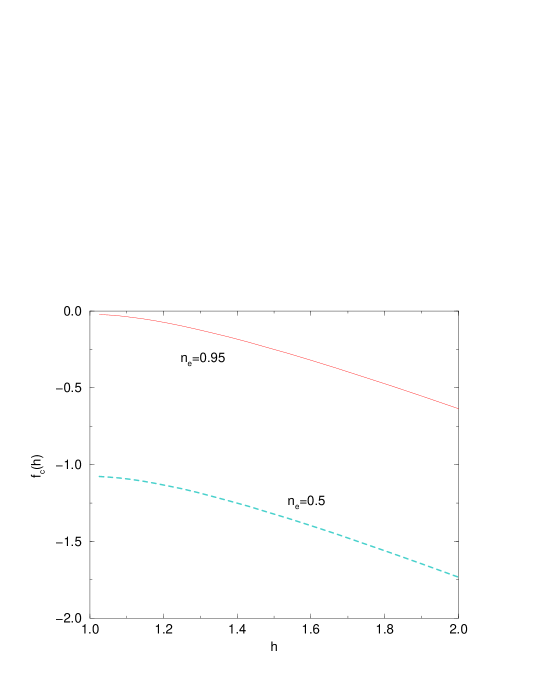
FIG. 3.: Energy of holon bound states as a function of boundary chemical potential.

This characterizes the relevant part of the low-lying finite-size spectrum of the open $t$-$J$ chain with boundary fields in the sector where $N_{\uparrow}\geq N_{\downarrow}$. In order to extract the X-ray exponents we need to consider states with $N_{\downarrow}\geq N_{\uparrow}$ for the case where the core electron carries spin down. This can be taken care of by changing the reference state of the Bethe Ansatz to the state with all spins down [18]. The result is of the same form as (25) but with redefined $\Delta N_{s}^{0}$.

We also need the finite-size ground state energy of the $t$-$J$ model with periodic boundary conditions. It is given by [16]

$$E^{(0)}=Le_{\infty}-\frac{\pi}{6L}(v_{c}+v_{s})\ .$$ (37)

We now have the necessary machinery to determine X-ray exponents. One should keep in mind that we presently have repulsive boundary fields. For pedagogical reason we nonetheless will calculate X-ray exponents for this case:

Absolute Threshold:The lowest (in frequency) threshold in the X-ray absorption intensity occurs at some frequency $\omega_{0}$ and is associated with an intermediate state in which both holon bound states are occupied. For the case where the core electron has spin up this corresponds to $\Delta N^{0}_{c}=-3\ ,\ \Delta N^{0}_{s}=-1$. Combining (25), (37), (10) and (11) we obtain

$$\alpha_{abs}=\frac{1}{2}-\frac{[3+\theta_{0}^{c}]^{2}}{2\xi^{2}}\ .$$ (38)

For the case where the core electron has spin down we need to proceed as outlined above and use the Bethe Ansatz solution with a different reference state. The final result is the same as (38) as $H_{\tt aa}$ preserves the discrete spin reversal symmetry.

Intermediate Thresholds:The second and third thresholds occur when one of the holon bound states is occupied but the other one is not. Let us consider the case where the bound state at $1$ is occupied. The corresponding threshold in the X-ray absorption rate is at $\omega_{0}-f_{c}(h_{1})$. As only one holon bound state is occupied we now have $\Delta N^{0}_{s}=-1,\ \Delta N^{0}_{c}=-2$ and the expressions for the quantities $\theta^{s,c}$ in (25) get modified. They are now given by (29) but with different driving terms

$$\theta_{1}^{s}=\frac{\theta_{1}^{c}}{2}+\frac{1}{2}\ ,\quad g_{c,1}(\lambda)=G_{1+S_{1}}(\lambda)+G_{1-S_{1}}(\lambda)-G_{0}(\lambda)-a_{S_{1}}-a_{s_{L}}\ .$$ (39)

The X-ray exponent associated with this threshold is

$$\alpha_{int}=\frac{1}{2}-\frac{[2+\theta_{1}^{c}]^{2}}{2\xi^{2}}\ .$$ (40)

Band Threshold:The fourth and final threshold occurs at $\omega_{0}-f_{c}(h_{L})-f_{c}(h_{1})$ when neither bound state is occupied. This corresponds to the case where the core electron is emitted into the conduction band where it decomposes into an antiholon and a spinon. Then $\Delta N^{0}_{c}=-1\ ,\ \Delta N^{0}_{s}=-1$, $\theta^{c}_{3}=2\theta^{s}_{3}$, $g_{c,3}(\lambda)=-G_{0}(\lambda)-a_{S_{1}}(\lambda)-a_{S_{L}}(\lambda)$ and the associated X-ray exponent is

$$\alpha_{band}=\frac{1}{2}-\frac{(1+\theta_{3}^{c})^{2}}{4\xi^{2}}\ .$$ (41)

B Attractive Boundary fields: $0\leq h\leq 1$

This region of boundary fields corresponds to an attractive core hole potential because of the form of the third last term in (13). Now no boundary bound states exist. The analysis of the finite-size spectrum follows the one above, the only difference being the absence of purely imaginary roots. The X-ray exponent is of the same form as (41) where we should keep in mind that $S_{1,L}$ now are negative. The results for two different band fillings are plotted in Fig. 4a as functions of the boundary chemical potential $h=h_{1}=h_{L}$.

(a) (b)

FIG. 4.: X-ray exponents (a) and ${\pi\theta^{c}}/{\xi^{2}}$ (b) for the $t$-$J$ model with aa boundary conditions and $h_{1}=h_{L}=h<1$.

Our result coincides with Refs. [10, 11] if we make the identification $\theta^{c}=\frac{V_{f}}{\pi}\xi^{2}$, where $V_{f}$ is the forward scattering amplitude of the core hole potential in the continuum limit. We see that $\theta^{c}$ does not vanish for $h_{1,L}\to 0$. As explained above the continuum $V_{f}$ is not simply given by the boundary chemical potential so that there is no contradiction. In Fig. 4b we plot ${\pi\theta^{c}}/{\xi^{2}}$ as a function of $h$.

C Attractive Boundary fields: $h\leq 0$

In this range of boundary chemical potential the analysis of the finite-size spectrum is less intuitive than above. The Bethe equations (17) allow a variety of boundary string solutions like the ones encountered in the repulsive case. However one finds that none of these complex roots is present in the ground state. We interpret this as follows: in the ground state antiholons and spinons are bound to the boundaries. States where some of these bound states are unoccupied are characterized by imaginary roots of the Bethe equations. In support of this interpretation we can compute the particle number at the boundary site. It is given by $\frac{\partial E}{\partial h}$, where $h$ is the boundary field. We find that in the ground state there is a strong enhancement of charge at the boundary site as compared to the bulk. The states involving imaginary roots of the Bethe equations exhibit a significant decrease in charge at the boundary as compared to the ground state, which is consistent with our interpretation.

Absolute Threshold:

In order to calculate the X-ray exponent for the lowest threshold we need the finite-size energy of the ground state for $h<0$. As no complex roots of the Bethe equations are present the analysis is straightforward and very similar to the band threshold for $2>h>1$. We find

$$\alpha_{abs}=\frac{1}{2}-\frac{(1+\theta^{c})^{2}}{2\xi^{2}}\ ,$$ (42)

where $\theta^{c}$ is given by (29) with $g_{c}(\lambda)=-G_{0}(\lambda)-a_{S_{1}}(\lambda)-a_{S_{L}}(\lambda)$.

In Fig. 5 the X-ray exponents of the absolute threshold are plotted as functions of the boundary chemical potential for two different band fillings. For simplicity we only consider the case $h_{1}=h_{L}=h$.

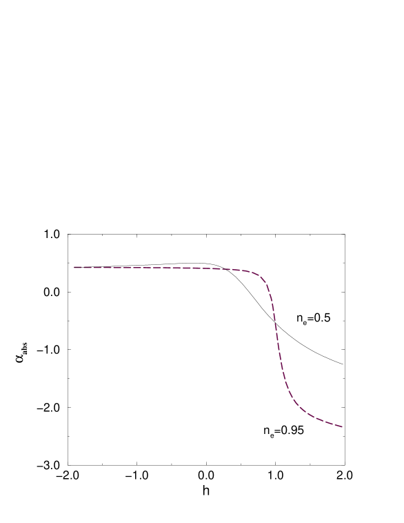
FIG. 5.: X-ray exponents for the absolute threshold in the $t$-$J$ model with $h_{1}=h_{L}=h$ at almost half-filling and quarter-filling.

We see that in the physical regime $h\leq 1$ there is always a singularity associated with the absolute threshold i.e. $I(\omega)$ always diverges.

Higher Thresholds:Let us consider the case in which two complex roots $\lambda^{(1)}$ are present and take the values $-\frac{i}{2}S_{1,L}$ respectively. The Bethe equations read

$$\left(e_{1}(\lambda_{\alpha})\right)^{2L}\prod_{j=1,L}e_{1-S_{j}}(\lambda_{\alpha})e_{1+S_{j}}(\lambda_{\alpha})$$ (43)

$$\qquad=\prod_{\beta\neq\alpha}^{N_{h}+N_{\downarrow}}e_{2}(\lambda_{\alpha}-\lambda_{\beta})e_{2}(\lambda_{\alpha}+\lambda_{\beta})\prod_{\gamma=1}^{N_{h}-2}e_{-1}(\lambda_{\alpha}-\lambda^{(1)}_{\gamma})e_{-1}(\lambda_{\alpha}+\lambda^{(1)}_{\gamma})$$ (44)

$$1=e_{-S_{1}}(\lambda^{(1)}_{\gamma})e_{-S_{L}}(\lambda^{(1)}_{\gamma})\prod_{\beta=1}^{N_{h}+N_{\downarrow}}e_{1}(\lambda^{(1)}_{\gamma}-\lambda_{\beta})e_{1}(\lambda^{(1)}_{\gamma}+\lambda_{\beta})\ .$$ (45)

Following through the same steps as before we find that this state has a gap of magnitude $\Delta f=f_{c}(S_{1})+f_{c}(S_{L})$ where

$$f_{c}(S)=\mu-\pi[G_{S+1}(0)-G_{S-1}(0)]+\frac{1}{2}\int_{-\Lambda_{c}}^{\Lambda_{c}}d\lambda\ \varepsilon_{c}(\lambda)[G_{S+1}(\lambda)-G_{S-1}(\lambda)]\ .$$ (46)

We interpret this state as differing from the ground state by leaving boundary bound states of antiholons unoccupied. Consequently we find a threshold in the X-ray absorption probability at a frequency $\Delta f$ higher than the absolute threshold with exponent

$$\alpha_{int}=\frac{1}{2}-\frac{(3+\theta^{c})^{2}}{2\xi^{2}}\ ,$$ (47)

where $\theta^{c}$ is given by (29) with $g_{c}(\lambda)=-G_{0}(\lambda)+\sum_{j=1,L}G_{S_{j}+1}(\lambda)-G_{S_{j}-1}(\lambda)-a_{S_{j}}(\lambda)$.

Thresholds at lower frequencies occur if we have only one imaginary root $\lambda^{(1)}=-\frac{i}{2}S$ where $S$ is either $S_{1}$ or $S_{L}$. The corresponding states have a gap equal to $\Delta f=f_{c}(S)$ and give rise to exponents

$$\alpha_{int}^{\prime}=\frac{3}{4}-\frac{(2+\theta^{c})^{2}}{2\xi^{2}}\ ,$$ (48)

where $\theta^{c}$ is given by (29) with $g_{c}(\lambda)=-G_{0}(\lambda)+G_{S+1(\lambda)}-G_{S-1}(\lambda)-a_{S_{1}}(\lambda)-a_{S_{L}}(\lambda)$. A numerical solution of the relevant integral equations for a quarter filled band shows that $\alpha_{int}$ is negative and therefore leads to a “shoulder” in $I(\omega)$ as in Fig. 1 b). On the other hand we find that $\alpha^{\prime}_{int}$ is positive and leads to a singularity.

The cases imvestigated above by no means exhaust the list of states with imaginary roots. For example there is a state with two imaginary $\lambda^{(1)}$’s taking the values $-\frac{i}{2}S_{1,L}$ and two imaginary $\lambda$’s taking the values $\frac{i}{2}(1-S_{1,L})$ respectively. This type of solution of the Bethe equation also gives rise to three thresholds as imaginary $\lambda$’s are only allowed if their respective “partner” $\lambda^{(1)}$ is present as well. The calculation of the X-ray exponents is completely analogous to the case treated above so that we omit it.

III The Hubbard model

The one dimensional Hubbard model with open boundary conditions of type aa (i.e. boundary chemical potentials only)

$$H=-\sum_{j=1}^{L-1}\sum_{\sigma}\left(c^{\dagger}_{j,\sigma}c_{j+1,\sigma}+c^{\dagger}_{j+1,\sigma}c_{j,\sigma}\right)+4u\sum_{j=1}^{L}n_{j\uparrow}n_{j\downarrow}+\mu\hat{N}-h_{1}n_{1}-h_{L}n_{L}\$$ (49)

is soluble by means of the Bethe Ansatz as shown in Refs. [21, 22] (note that the boundary potentials are defined in a different way than above: to identify $h_{1,L}$ in (49) with those used for the $t$–$J$ model one should replace $h_{1,L}\to 1-h_{1,L}$). Applying boundary magnetic fields instead also leaves the Hubbard model integrable [23] but will not be considered here. The Bethe Ansatz equations determining the spectrum of (49) in the $N_{e}$-particle sector with magnetization $M={1\over 2}N_{e}-N_{\downarrow}$ read [21, 22]

$$e^{2ik_{j}L}B^{(1)}_{c}(k_{j})B^{(L)}_{c}(k_{j})=\prod_{\beta=1}^{N_{\downarrow}}e_{2u}(\sin k_{j}-\lambda_{\beta})e_{2u}(\sin k_{j}+\lambda_{\beta})\ ,\qquad j=1,\ldots,N_{e}$$ (50)

$$B^{(1)}_{s}(\lambda_{\alpha})B^{(L)}_{s}(\lambda_{\alpha})\prod_{j=1}^{N_{e}}e_{2u}(\lambda_{\alpha}-\sin k_{j})e_{2u}(\lambda_{\alpha}+\sin k_{j})$$ (51)

$$\qquad=\prod_{\beta\neq\alpha}^{N_{\downarrow}}e_{4u}(\lambda_{\alpha}-\lambda_{\beta})e_{4u}(\lambda_{\alpha}+\lambda_{\beta})\ ,\qquad\alpha=1,\ldots,N_{\downarrow}.$$ (52)

The quasi momenta $k_{j}$ and the spin rapidities $\lambda_{\alpha}$ paramatrize an eigenstate of (49) with energy

$$E=\mu N_{e}-2\sum_{j=1}^{N_{e}}\cos k_{j}\ .$$ (53)

For small values of the boundary fields the ground state configuration is given by distributions of real $k_{j}$ and $\lambda_{\alpha}$ and

$$B^{(x)}_{c}(k)=\left({{e^{ik}-h_{x}}\over{1-h_{x}e^{ik}}}\right)\ ,\qquad B^{(x)}_{s}(\lambda)=1\ ,$$ (54)

contain the phase shifts due to the boundaries (this case has been discussed in Ref. [22]). For sufficiently large boundary chemical potentials $h_{1,L}$, however, the Bethe Ansatz equations (52) allow for various complex solutions corresponding to boundary bound states for antiholons, spinons and pairs of electrons, respectively [24]: First, for $h_{1,L}>1$ one finds bound states parametrized by $k=i\ln h_{1,L}$ with exponential accuracy in the thermodynamic limit $L\to\infty$. The quasi momenta parametrize the charge part of the states: hence this solution corresponds to a charge (or antiholon) bound to the surface. Inserting this solution in the second set of Eqs. (52) leads to a boundary phase shift in addition to the product over the real quasi momenta $k_{j}$ which modifies $B_{s}$ ($B_{c}$ remains unchanged):

$$B^{(x)}_{s}(\lambda)=e_{2(u+S_{x})}(\lambda)\ e_{2(u-S_{x})}(\lambda)\ ,$$ (55)

where we have introduced $S_{x}=(h_{x}-1/h_{x})/2>0$ with $x=1$ or $L$. Analyzing the resulting equations we find that a new type of solution arises at $S_{x}=u$, i.e. $h_{x}=u+\sqrt{u^{2}+1}$: Beyond this point a complex solution $\lambda=i(S_{x}-u)$ for the spin rapidities is allowed. We note that spinons are to be identified with holes in the distribution of spin rapidities. Again, occupation of this state modifies the boundary phase shifts $B_{c,s}$:

$$B^{(x)}_{c}(k) = \left({{e^{ik}-h_{x}}\over{1-h_{x}e^{ik}}}\right)e_{-2S_{x}}(\sin{}k_{j})e_{2(S_{x}-2u)}(\sin{}k_{j})\ ,$$ (56)

$$B^{(x)}_{s}(\lambda) = e_{2(S_{x}-3u)}(\lambda)\ e_{2(u-S_{x})}(\lambda)\ .$$ (57)

Finally, boundary potentials with $S_{x}>2u$ can bind a (singlet) pair of electrons to site $x$. Such a state is parametrized by two complex quasi momenta $\sin{}k_{0}^{(\pm)}=\lambda_{0}\pm iu$ and a single complex spin rapidity $\lambda_{0}=i(S_{x}-u)$ as before. The remaining real solutions of the Bethe Ansatz equations are determined by (52) with

$$B^{(x)}_{c}(k)=\left({{e^{ik}-h_{x}}\over{1-h_{x}e^{ik}}}\right)e_{-2S_{x}}(\sin{}k_{j})e_{2(S_{x}-2u)}(\sin{}k_{j})\ ,\qquad B^{(x)}_{s}(\lambda)=1\ .$$ (58)

Depending on the strength of the boundary potential we have to distinguish between the following cases in order to describe the spectrum: in addition to the case discussed in Ref. [22], where the solution of the Bethe Ansatz eqs. is given in terms of real $k_{j}$ and $\lambda_{\alpha}$ only, one can find either

• an antiholon in a bound state (corresponding to a complex $k$) and the spinon in the corresponding band (which implies the presence of a complex $\lambda$ for $S_{x}>u$),

• an antiholon and a spinon in bound states (parametrized by a complex $k$ for $S_{x}>u$),

• and finally, for $S_{x}>2u$, a pair of electrons bound by the potential.

Each of these configurations gives rise to a continuous spectrum above a threshold that depend on the occupation of the boundary states.

In the following, we shall discuss some of these cases for the symmetric choice $h_{1}=h_{L}=h$ of the boundary potentials. The bound states discussed above will occur pairwise at the given thresholds (corresponding to sites $1$ and $L$, respectively). As for the $t$–$J$ model we shall consider the logarithmic form of the Bethe Ansatz equations (52) for low lying states above these thresholds:

$${2\pi I_{j}\over L} = 2k_{j}+{1\over L}\sum_{\beta=1}^{M}\left\{\theta\left({\sin k_{j}-\lambda_{\beta}\over 2u}\right)+\theta\left({\sin k_{j}+\lambda_{\beta}\over 2u}\right)\right\}+{1\over L}\kappa(k_{j})\ ,\qquad j=1,\ldots,N$$ (59)

$${2\pi J_{\alpha}\over L} = {1\over L}\sum_{j=1}^{N}\left\{\theta\left({\lambda_{\alpha}-\sin k_{j}\over 2u}\right)+\theta\left({\lambda_{\alpha}+\sin k_{j}\over 2u}\right)\right\}$$ (61)

$$-{1\over L}\sum_{\beta\neq\alpha}^{M}\left\{\theta\left({\lambda_{\alpha}-\lambda_{\beta}\over 4u}\right)+\theta\left({\lambda_{\alpha}+\lambda_{\beta}\over 4u}\right)\right\}+{1\over L}\omega\left(\lambda_{\alpha}\right)\ ,\qquad\alpha=1,\ldots,M\ .$$

Here the summations extend over the real roots $k_{j}$ and $\lambda_{\alpha}$. The functions $\kappa$ and $\omega$ contain the phase shifts due to the boundary fields and occupation of the boundary bound states.

A Band threshold

The edge singularity with the highest threshold corresponds to excitation in states with no bound states occupied by the particles. This situation was studied in Ref. [22]. Like in the case of the $t$–$J$ model this does in fact imply the occupation of a holon bound state for repulsive boundary potentials $h_{1,L}<-1$: computation of the particle number on the boundary site shows a depletion due to the presence of the holon[24]. In the Bethe Ansatz equations the only boundary phase shifts are those due to the boundary potentials, i.e. (54). The resulting $\kappa(k)$ in (61) is given by

$$\kappa(k)=-2i\ln\left({{e^{ik}-h}\over{1-he^{ik}}}\right),$$ (62)

while $\omega(\lambda)=0$. The finite size spectrum for the relevant boundary conditions is again given by (25) and (37) [25, 22]. The dressed charge $\xi=\xi(Q)$ for the Hubbard model is defined in terms of the solution of the integral equation ($Q$ varies between $0$ and $\pi$ as a function of the density of electrons and the coupling constant) [25, 15]

$$\xi(k) = 1+\int_{-Q}^{Q}dk^{\prime}\cos{}k^{\prime}\ {\bar{K}}(\sin{}k-\sin{}k^{\prime})\xi(k^{\prime})\ ,$$ (63)

$${\bar{K}}(x) = {1\over 2\pi}\int_{0}^{\infty}d\omega{e^{-u\omega}\over\cosh{}u\omega}\cos{}\omega x\ .$$ (64)

Here $\theta^{c,s}$ are related via $\theta^{s}={1\over 2}\theta^{c}$ with

$$\theta^{c}={1\over 2}\left(\int_{-Q}^{Q}dk\rho_{c}^{(1)}(k)\ -1\right)$$ (65)

for our choice of the reference state. The $O(1/L)$ contribution $\rho_{c}^{(1)}$ to the density from the boundary fields is given in terms of the integral equation

$$\rho_{c}^{(1)}(k)={\bar{g}}_{c}(k)+\cos{}k\ \int_{-Q}^{Q}dk^{\prime}{\bar{K}}(\sin{}k-\sin{}k^{\prime})\rho_{c}^{(1)}(k^{\prime})\ .$$ (66)

For the case considered here the driving term in this equation is found to be (after integrating out the spinon-part of the densities)

$${\bar{g}}_{c}(k)={\bar{g}}_{c}^{(0)}(k)={1\over\pi}\ {1-h^{2}\over 1+h^{2}-2h\cos{}k}-{\cos{}k\over 4u\cosh({\pi\over 2u}\sin{}k)}\ .$$ (67)

An analytic solution of this integral equation is possible in certain limits only. It simplifies essentially in the strong coupling limit where ${\bar{K}}(x)\equiv\ln 2/2\pi u$. This allows to give a simpler expression for $\theta^{c}$ in terms of the driving term

$$\theta^{c}\simeq{1\over 2}\left[\left(1+{\ln 2\over\pi u}\sin Q\right)\int_{-Q}^{Q}dk{\bar{g}}_{c}(k)\ -1\right]\ \quad{\mathrm{f}or~{}}u\to\infty\ .$$ (68)

Furthermore it is known that $Q=\pi n_{c}$ and $\xi=1$ in this limit. With (67) we find

$$\theta^{c}={2\over\pi}\arctan\left({1+h\over 1-h}\tan{\pi n_{c}\over 2}\right)-{1\over 2}\$$ (69)

for infinite coupling [26]. In general the integral equations have to be solved numerically to compute the X-ray edge exponents from (10) by comparing (25) to the finite size ground state energy of the Hubbard chain with periodic boundary conditions (37). For absorption of the core electron into the band we have to choose $\Delta N_{c}^{0}=1$. The number of down spins in the system changes by $\Delta N_{s}^{0}=0$ or $1$ depending on the spin of the core electron. Without magnetic fields the Bethe Ansatz states are highest weight in the spin $SU(2)$, i.e. correspond to the first case. This results in the following expression for the exponent

$$\alpha_{band}={1\over 2}-{1\over 2\xi^{2}}\left(\theta^{c}-1\right)^{2}\ .$$ (70)

From (69) we find that there is a discontinuity of $\alpha_{band}(h)$ at $h=1$: at this point the charge bound state first appears leading to a jump of the exponent from ${3/8}$ to ${-21/8}$ at $u=\infty$ (note that small negative exponents correspond to a ‘shoulder’ rather than a singularity in the absorption profile [3], exponents $\alpha<-1$ will hardly lead to an observable feature). Large boundary potentials $h\to\pm\infty$ lead to $\theta^{c}\to-(n_{c}+{1\over 2})$ in the strong coupling limit giving $\alpha_{band}\to-{1\over 2}(n_{c}^{2}+3n_{c}+{5\over 4})$ which is always negative. Numerical solutions of the equations show a similar behaviour for finite $u$ (see Fig. 6).

FIG. 6.: X-ray edge exponents for band absorption (full line) and photoemission (dashed line) in the Hubbard model as a function of the boundary chemical potential $h$ for $u=1$, $n_{e}=0.5$.

Similarly, the singularity of the absorption intensity measured in a photoemission experiment is given by a power law with exponent obtained from (10) with $\Delta N_{cs}^{0}=0$:

$$\alpha_{photo}={3\over 4}-{1\over 2\xi^{2}}\left(\theta^{c}\right)^{2}\ ,$$ (71)

which exhibits a jump from $5/8$ to $-3/8$ at $h=1$ and approaches ${5\over 8}-{1\over 2}n_{c}(n_{c}+1)$ at $h\to\infty$ for infinite coupling. Note that $(1/2\xi^{2})$ varies as a function of the bulk density $n_{e}$ of electrons and the interaction strength between $1/4$ for noninteracting fermions and $1/2$ in the infinite $u$ limit of the Hubbard model [15], while $\theta^{c}$ contains the dependence on the strength of the boundary potentials $h_{1,L}$ (in addition to $n_{c}$ and $u$).

For weak boundary fields $h<1$ these expressions coincide with those found in the framework of a bosonized theory of spin carrying electrons [11, 10] provided that we identify $\theta^{c}$ with the forward scattering amplitude of the core hole potential (see also the discussion at the beginning of Sect. II).

B Absolute threshold

Let us now consider X-ray processes which excite the system into the sector with all bound states occupied, i.e. the absolute threshold for absorption. Following the discussion above one has to distinguish four cases: For sufficiently small boundary fields ($h<1$) there are no bound states, which is the situation considered in the previous section.

For boundary fields $1<h<u+\sqrt{u^{2}+1}$ a charge can be bound to either boundary. This changes the boundary phase shifts according to (55). The computation of the finite size spectrum is complete analogeous to the case considered above and results in (25). The shifts of the numbers $\Delta N_{cs}^{0}$ are now found to be $\theta^{s}={1\over 2}\theta^{c}+1$ and $\theta^{c}$ again given by (65). The different boundary phase shifts modify the driving term in (66) to

$${\bar{g}}_{c}(k)={\bar{g}}_{c}^{(0)}(k)+\cos{}k\ f_{b}(\sin{}k)$$ (72)

with

$$f_{b}(x)=2a_{2(2u-S)}(x)+{1\over u}\left\{G_{1+{S\over u}}\left({x\over 2u}\right)-G_{3-{S\over u}}\left({x\over 2u}\right)\right\}\ .$$ (73)

For the computation of the edge exponent from (25) we have to choose $\Delta N_{c}^{0}=-1$ (the number of charges in the band is increased by one due to the absorption of the core electron, but at the same time two of the band electrons occupy the bound states in the final state). With $\Delta N_{s}^{0}=0$ as before one obtains

$$\alpha_{abs}={1\over 2}-{1\over 2\xi^{2}}\left(\theta^{c}+1\right)^{2}\ .$$ (74)

Increasing the boundary potentials such that $u+\sqrt{u^{2}+1}<h<2u+\sqrt{4u^{2}+1}$ the Bethe Ansatz state of lowest energy is contains both complex $k$ and complex $\lambda$ leading to phase shifts (57). As discussed above this corresponds to occupied charge bound states while the spinon bound states are empty. Analysing the Bethe Ansatz equations we find $\theta^{s}={1\over 2}\theta^{c}-1$. The function $\rho_{c}^{(1)}(k)$ is determined by the same set of equations (66), (72) and (73) as above. The state relevant for the edge exponent is now determined by the quantum numbers $\Delta N_{c}^{0}=-1$ and $\Delta N_{s}^{0}=-2$ which gives again (74).

A final change in the configuration describing the absolute ground state occurs for $h>2u+\sqrt{4u^{2}+1}$ ($S>2u$). The presence of bound pairs of electrons leads to the phase shifts (58) in the Bethe Ansatz equations. The quantities determining the edge exponents are now $\theta^{s}={1\over 2}\theta^{c}$, where $\theta^{c}$ has to be computed from (66) with

$${\bar{g}}_{c}(k)={\bar{g}}_{c}^{(0)}(k)+2\cos{}k\left\{a_{2S}(\sin{}k)-a_{2(S-2u)}(\sin{}k)\right\}\ .$$ (75)

The quantum numbers of the final state are $\Delta N_{c}^{0}=-3$ and $\Delta N_{s}^{0}=-2$ which gives

$$\alpha_{abs}={1\over 2}-{1\over 2\xi^{2}}\left(\theta^{c}+3\right)^{2}\ .$$ (76)

Again, the equations simplify significantly in the strong coupling limit where one should rescale $S$ by $u$ to see the different regimes. Using (68) we can combine Eqs. (70), (74) and (76) into $\alpha_{abs}={1\over 2}\left(1-x^{2}\right)$ where

$$x={2\over\pi}\left\{\arctan\left({{h-\cos\pi n_{c}}\over{\sin\pi n_{c}}}\right)+\arctan\left({{h-4u}\over{2\sin\pi n_{c}}}\right)\right\}-n_{c}+{1\over 2}\ .$$ (77)

Hence we find the following expression for the edge exponent of the absolute threshold in the strong coupling limit

$$\alpha_{abs}\to\left\{\begin{array}[]{cl}-{1\over 8}(2n_{c}+5)(2n_{c}+1)&{\mathrm{~{}}for~{}}h\ll-1\\[4.0pt] -{1\over 8}(2n_{c}+1)(2n_{c}-3)&{\mathrm{~{}}for~{}}1\ll h\ll 4u\\[4.0pt] -{1\over 8}(2n_{c}-3)(2n_{c}-7)&{\mathrm{~{}}for~{}}h\gg 4u\end{array}\right.\ .$$ (78)

Since we consider the Hubbard model at less than half filling (i.e. $n_{c}<1$) this implies that a positive exponent $\alpha$ leading to a edge singularity is possible only in the intermediate regime. The corresponding numerical data for finite $u$ are presented in Figure 7.

FIG. 7.: Exponents at the absolute threshold for X-ray absorption in the Hubbard model as a function of the boundary chemical potential $h$ for $u=1$ and several densities $n_{c}$.

C Intermediate thresholds

Finally we consider some cases where the absorption excites the system into a state in which some but not all bound states are occupied. First, let the final state be characterized by one antiholon and one spinon in a bound state which gives rise to a singularity at an energy between the two thresholds discussed above. Such a process is possible for boundary potentials $h>u+\sqrt{u^{2}+1}$ (or $S>u$) and corresponds to a Bethe Ansatz state with a single complex $k$. Analyzing the Bethe Ansatz equations we obtain the relation $\theta^{s}={1\over 2}\theta^{c}$. In this case $\theta^{c}$ has to be computed from Eqs. (65) and (66) with ${\bar{g}}_{c}(k)$ given by (72) with

$$f_{b}(x)=-a_{2S}(x)+{1\over u}G_{{S\over u}+1}\left({x\over 2u}\right).$$ (79)

The finite size spectrum is again of the form (25); the quantum numbers of the relevant final state are $\Delta N_{c}^{0}=0=\Delta N_{s}^{0}$. From (10) we obtain

$${\alpha}_{int}={3\over 4}-{1\over 2\xi^{2}}\left(\theta^{c}\right)^{2}$$ (80)

for the edge exponent determining the singularity at this threshold. In the strong coupling limit we find that ${\alpha}_{int}$ varies between $5/8$ for the empty band and $-3/8$ as we approach half-filling. An edge singularity can be observed for $n_{c}<\sqrt{{3\over 2}}-{1\over 2}\approx 0.725$.

A different intermediate thershold occurs if only an antiholon is in one of the bound states. This final state is already possible for $h>1$ and is parametrized by a single complex root $k=i\ln h$ for $S<u$ and an additional complex spin rapidity $\lambda$ for $S>u$. Depending on $h$ several cases have to be distinguished resulting in a edge singularity with exponent

$${\alpha}_{int}^{\prime}={1\over 2}-{1\over 2\xi^{2}}\left(\theta^{c}\right)^{2}\$$ (81)

for $S<3u$ (for $S>3u$ the exponent is always negative). The function $f_{b}(x)$ in (72) is now simply one half of that in (73). In the strong coupling limit the edge exponent ${\alpha}_{int}^{\prime}$ can be expressed through $n_{c}$ and $h$ using Eq. (69). In this limit a singularity in the absorption spectrum (i.e. positive exponent) can be observed for sufficiently large boundary potentials $h\gtrsim\tan\left({\pi\over 4}(2n_{c}+1)\right)>1$ as long as $n_{c}<{1\over 2}$ but only close to $h\approx 4u$ above quarter filling.

Note that for sufficiently strong boundary potentials the cases discussed here are only a small subset of the possible thresholds. Furthermore, for sufficiently strong repulsive boundary potentials, i.e. $h<-1$, the spectrum allows for holon bound states. Like in the case of the $t$-$J$ model with attractive boundary chemical potentials there exist solutions to the Bethe equations with complex quasi momenta $k=\pi+i\ln|h|$ of Eq. (52) that have a gap with respect to the absolute ground state and lead to a higher threshold in the X-ray spectrum.

IV Conclusions

In this work we have determined the X-ray edge exponents in a Luttinger liquid for the case where the local disturbance due to the core hole leads to bound states. We used specific realizations of Luttinger liquids on the lattice, namely Hubbard and $t$-$J$ models with integrable boundary terms. The main difference to the Fermi liquid case (1) solved in Refs. [3, 5] is that due to spin and charge separation we find a richer structure of thresholds in the X-ray absorption rate associated with bound states of spinons and (anti)holons. Using Boundary Conformal Field Theory the exact dependence of the edge exponents on band filling and interaction strength can be extracted from the finite size spectra which are determined from the Bethe Ansatz solution.

For weak boundary fields our results coincide with those obtained in a field theoretical treatment by Prokof’ev[10] and Affleck and Ludwig[11] if the boundary chemical potentials are fine-tuned.

For sufficiently strong boundary fields the models considered in this paper allow for various bound states, each of which can lead — in principle — to a singularity in the absorption spectrum. Previous studies of these additional singularities have not taken into account the interaction between the particles in the bound states and those remaining in the band [3, 5]. This results in a simple relation between the exponents at different edges with the phase shift $\delta(\epsilon_{F})$ at the Fermi surface as the only free parameter. In the systems considered here the occupation of the boundary bound states modifies the potential acting on the particles remaining in the bands which in turn modifies the corresponding phase shifts. Examining the edge exponents for the different thresholds we find that for generic values of boundary potentials and filling factors many of them will in fact be negative, and consequently won’t lead to an observable singularity in the spectrum.

REFERENCES

- [1] P. Nozières and C. T. de Dominicis, Phys. Rev. 178, 1097 (1969).
- [2] K. D. Schotte and U. Schotte, Phys. Rev. 182, 479 (1969).
- [3] M. Combescot and P. Nozières, J. Physique 32, 913 (1971).
-
[4]
D. B. Abraham, E. Barouch, G. Gallavotti, and A. Martin-Löf, Stud. Appl.
Math. LI, 211 (1972);
E. Barouch, B. M. McCoy, and M. Dresden, Phys. Rev. A 2, 1075 (1970). - [5] I. Affleck, preprint hep-th/9611064.
- [6] V. E. Korepin, A. G. Izergin, and N. M. Bogoliubov, Quantum Inverse Scattering Method, Correlation Functions and Algebraic Bethe Ansatz (Cambridge University Press, 1993).
- [7] Exactly Solvable Models of Strongly Correlated Electrons, edited by V. E. Korepin and F. H. L. Eßler (World Scientific, Singapore, 1994).
- [8] A. Gogolin, A. Nersesyan and A. M. Tsvelik, Bosonization (Cambridge University Press, to appear).
-
[9]
T. Ogawa, A. Furusaki, and N. Nagaosa, Phys. Rev. Lett. 68, 3638
(1992);
D. K. K. Lee and Y. Chen, Phys. Rev. Lett. 69, 1399 (1992). - [10] N. V. Prokof’ev, Phys. Rev. B 49, 2148 (1994).
- [11] I. Affleck and A. W. W. Ludwig, J. Phys. A 27, 5375 (1994).
-
[12]
J. L. Cardy, Nucl. Phys. B 324, 581 (1989);
I. Affleck, in Correlation effects in low-dimensional electron systems, Vol. 118 of Springer Series in Solid-State Sciences, edited by A. Okiji and N. Kawakami (Springer Verlag, Berlin, 1994), pp. 82–95. - [13] I. Peschel and K. D. Schotte, Z. Phys. B 54 (1984), 305 (1984).
-
[14]
C. L. Kane and M. P. A. Fisher, Phys. Rev. B 46, 7268 (1992);
S. Qin, M. Fabrizio, and L. Yu, Phys. Rev. B 54, R9643 (1996);
S. Eggert and I. Affleck, Phys. Rev. B 46, (10866);
A. Luther and I. Peschel, Phys. Rev. Lett. 32, 992 (1974);
D. C. Mattis, Phys. Rev. Lett. 32, 714 (1974). - [15] H. Frahm and V. E. Korepin, Phys. Rev. B 42, 10533 (1990).
- [16] N. Kawakami and S.-K. Yang, J. Phys. Condens. Matter 3, 5983 (1991).
- [17] A. G. Izergin, V. E. Korepin, and N. Yu. Reshetikhin, J. Phys. A 22, 2615 (1989).
- [18] F. H. L. Eßler, J. Phys. A 29, 6183 (1996).
- [19] A. Kapustin and S. Skorik, J. Phys. A 29, 1629 (1996).
- [20] H. Asakawa and M. Suzuki, preprint (1996).
- [21] H. Schulz, J. Phys. C 18, 581 (1985).
- [22] H. Asakawa and M. Suzuki, J. Phys. A 29, 225 (1996).
-
[23]
M. Shiroishi and M. Wadati, J. Phys. Soc. Japan 66, 1 (1997);
T. Deguchi and R. Yue, preprint (1996). - [24] G. Bedürftig and H. Frahm, preprint ITP-UH-5/97.
- [25] F. Woynarovich, J. Phys. A 22, 4243 (1989).
- [26] H. Frahm and A. A. Zvyagin, Phys. Rev. B 55, 1341 (1997).