ITP-UH-5/97 February 1997

Spectrum of boundary states in the open Hubbard chain

Gerald Bedürftig and Holger Frahm

Institut für Theoretische Physik, Universität Hannover
D-30167 Hannover, Germany

We use the Bethe Ansatz solution for the one dimensional Hubbard model with open boundary conditions and applied boundary fields to study the spectrum of bound states at the boundary. Depending on the strength of the boundary potentials one finds that the true ground state contains a single charge or, for boundary potentials comparable to the Hubbard interaction, a pair of electrons in a bound state. If these are left unoccupied one finds holon and spinon bound states. We compute the finite size corrections to the low lying energies in this system and use the predictions of boundary conformal field theory to study the exponents related to the orthogonality catastrophe.

PACS-Nos.: 05.70.Jk, 71.10.Fd, 71.10.Pm, 73.20.-r

1 Introduction

The recent advances in the understanding of boundary effects in low dimensional quantum systems due to the predictions of boundary conformal field theory [1, 2, 3] and the formulation of Bethe Ansatz soluble models on open lattices with potentials applied on the boundary sites [4, 5, 6, 7] have opened new possibilities to study the effects of correlations and quantum fluctuations on long standing problems such as the orthogonality catastrophe [8, 9] and edge singularities in optical absorption experiments [10, 11, 12].

The effect of electronic correlations on the bulk critical behaviour of $(1+1)$-dimensional quantum systems has been studied successfully in the Tomonaga-Luttinger model which then can be handled using field theoretical methods [13, 14, 15]. Studies of integrable lattice models have added insights to this problem since e.g. the dependence of critical exponents on microscopic parameters and their behaviour due to lattice effects (back scattering, Mott transition) can be computed exactly [16, 17, 18]. Similarly, one expects additional information from studies of lattice models for interacting electrons with open boundaries [4, 19, 20]. Besides giving a deeper understanding of previous predictions these lattice models have features not easily included into the continuum description: local chemical potentials in the former lead to a sequence of bound states (see e.g. [21]) which are expected to influence the critical properties of the boundary.

In this paper we consider the Hubbard model on a chain of $L$ sites subject to an additional chemical potential $p$ at the first site. The Hamiltonian is given by

$${\cal H}=-\sum_{\sigma,j=1}^{L-1}\left(c_{j,\sigma}^{\dagger}c_{j+1,\sigma}+h.c.\right)+4u\sum_{j=1}^{L}n_{j\uparrow}n_{j\downarrow}+\mu\hat{N}-{h\over 2}(\hat{N}-2\hat{N}_{\downarrow})-p(\hat{N}_{1,\uparrow}+\hat{N}_{1,\downarrow}).$$ (1.1)

For $p=0$ this model has been solved by Schulz using the coordinate Bethe Ansatz [4]. Only recently, this solution has been extended to nonvanishing $p$ [19] and the integrability of the model has been established in the framework of the quantum inverse scattering method [22]. The Bethe Ansatz equations (BAE) determining the spectrum of (1.1) in the $N_{e}$-particle sector with magnetization $M={1\over 2}N_{e}-N_{\downarrow}$ read [19]

$$e^{ik_{j}2(L+1)}s_{p}(k_{j}) = \prod_{\beta=1}^{N_{\downarrow}}e_{2u}(\eta_{j}-\lambda_{\beta})e_{2u}(\eta_{j}+\lambda_{\beta})\qquad j=1,\ldots,N_{e}$$

$$\prod_{j=1}^{N_{e}}e_{2u}(\lambda_{\alpha}-\eta_{j})e_{2u}(\lambda_{\alpha}+\eta_{j}) = \prod_{\beta=1\atop\beta\not=\alpha}^{N_{\downarrow}}e_{4u}(\lambda_{\alpha}-\lambda_{\beta})e_{4u}(\lambda_{\alpha}+\lambda_{\beta})\qquad\alpha=1,\ldots,{N_{\downarrow}}.$$

with $e_{n}(x)=\frac{x+i{n\over 2}}{x-i{n\over 2}}$, $s_{p}(k_{j})=\left(\frac{1-pe^{-ik_{j}}}{1-pe^{ik_{j}}}\right)$ and $\eta_{j}=\sin{}k_{j}$. The energy of the corresponding eigenstate of (1.1) is

$$E=\sum_{j=1}^{N_{e}}\left(\mu-{h\over 2}-2\cos{}k_{j}\right)+hN_{\downarrow}\ .$$ (1.3)

Using the global spin- and $\eta$–pairing SU(2) symmetry of the Hubbard model the Bethe states extended by those obtained by application of the corresponding raising operators have been shown to form a complete basis of the Hilbert space of the system [23]. A non-zero boundary potential destroys the $\eta$–symmetry of the model and the question of completeness should be considered again. Numerical solutions of (LABEL:eq:bae) for small $p$ show that there exist complex combinations of two $k$ and one $\lambda$ which coincide with one $\eta$–pair in the limit of $p\to 0$. In the following we only consider the ground state and the low lying excitations of the system, so we can neglect these kind of complex solutions as they belong to the highly excited states of the system [24]. However, for sufficiently strong attractive boundary potentials $p>1$ we find that there exist other complex solutions which turn out to correspond to bound states in these potentials (note that these states do not appear in the case $p<1$ studied in [19]). These solutions need to be considered to obtain the true ground state of the system. We find that in spite of the presence of several complex parameters in the ground state configuration the low–energy spectrum of the many particle system can still be described in the Tomonaga–Luttinger picture equivalent to two $c=1$ Conformal Field Theories. The case $p>1$ will be studied in detail in the next section.

2 Boundary bound states

From a physical point of view it is clear that the ground state of the model contains a bound state at the first site for sufficiently large $p$. Numerical solutions of the BAE show that this is indeed the fact for $p>1$ where a complex quasi momentum $k$ is present in the ground state configuration. A similar situation has been found in the XXZ Heisenberg chain with a boundary magnetic field [21, 25] and in a continuum model related to the Kondo problem [26].

Increasing the boundary potential further we find that additional complex parameters are added to the gound state solution of (LABEL:eq:bae). In the thermodynamic limit $(L\to\infty)$ we have to distinguish three different regions where the BAE describing the ground state are modified due to the presence of these complex roots:

• $1<p<p_{1}=u+\sqrt{1+u^{2}}$

  $$e^{ik_{j}2(L+1)}s_{p}(k_{j})=\prod_{\beta=1}^{N_{\downarrow}}e_{2u}(\eta_{j}-\lambda_{\beta})e_{2u}(\eta_{j}+\lambda_{\beta})\ ,\qquad j=1,\ldots,N_{e}-1$$

  $$e_{2u-2t}(\lambda_{\alpha})e_{2u+2t}(\lambda_{\alpha})\prod_{j=1}^{N_{e}-1}e_{2u}(\lambda_{\alpha}-\eta_{j})e_{2u}(\lambda_{\alpha}+\eta_{j})=\prod_{\beta=1\atop\beta\not=\alpha}^{N_{\downarrow}}e_{4u}(\lambda_{\alpha}-\lambda_{\beta})e_{4u}(\lambda_{\alpha}+\lambda_{\beta})\ ,$$

  $$\qquad\alpha=1,\ldots,{N_{\downarrow}}$$ (2.1)

  with the complex solution $k_{N_{e}}=i\ln(p)$ (with exponential accuracy in the limit $L\to\infty$) and $t=-i\sin{}k_{N_{e}}={1\over 2}(p-{1\over p})<u$. The contribution of this bound state to the energy (1.3) is given by $E_{1}=-p-{1\over p}+\mu-{h\over 2}$. This complex solution corresponds to a charge bound to the first site, as the quasimomenta $k$ parametrize the charge part of the states.

• $p_{1}<p<p_{2}=2u+\sqrt{1+4u^{2}}$
  Larger values of the boundary potential lead to an additional complex solution in the spin part: $\lambda_{N_{\downarrow}}=i(t-u)$ ($t>u$ in this region) and the following modified BAE:

  $$e^{ik_{j}2(L+1)}s_{p}(k_{j})=e_{4u-2t}(\eta_{j})e_{2t}(\eta_{j})\prod_{\beta=1}^{{N_{\downarrow}}-1}e_{2u}(\eta_{j}-\lambda_{\beta})e_{2u}(\eta_{j}+\lambda_{\beta})\ ,\qquad j=1,\ldots,N_{e}-1$$

  $$\prod_{j=1}^{N_{e}-1}e_{2u}(\lambda_{\alpha}-\eta_{j})e_{2u}(\lambda_{\alpha}+\eta_{j})=e_{2t-2u}(\lambda_{\alpha})e_{6u-2t}(\lambda_{\alpha})\prod_{\beta=1\atop\beta\not=\alpha}^{{N_{\downarrow}}-1}e_{4u}(\lambda_{\alpha}-\lambda_{\beta})e_{4u}(\lambda_{\alpha}+\lambda_{\beta})\ ,$$

  $$\qquad\alpha=1,\ldots,{N_{\downarrow}}-1$$ (2.2)

  Again, this state can be interpreted as that of a charge bound to the surface. The physical excitations in the spin sector — so called spinons — correspond to holes in the distribution of spin rapidities $\lambda$ which are still real.

• $p>p2$
  For boundary potentials larger than the Hubbard interaction $p\gtrapprox 4u$ a pair of electrons forming a singlet is bound to the surface, parametrized by $\lambda_{N_{\downarrow}}=\sin{}k_{N_{e}}\ -iu=\sin{}k_{N_{e}-1}\ +iu=i(t-u)$. The resulting BAE are

  $$e^{ik_{j}2(L+1)}s_{p}(k_{j})e_{2t-4u}(\eta_{j}) = e_{2t}(\eta_{j})\prod_{\beta=1}^{{N_{\downarrow}}-1}e_{2u}(\eta_{j}-\lambda_{\beta})e_{2u}(\eta_{j}+\lambda_{\beta})\qquad j=1,\ldots,N_{e}-2$$

  $$\prod_{j=1}^{N_{e}-2}e_{2u}(\lambda_{\alpha}-\eta_{j})e_{2u}(\lambda_{\alpha}+\eta_{j}) = \prod_{\beta=1\atop\beta\not=\alpha}^{{N_{\downarrow}}-1}e_{4u}(\lambda_{\alpha}-\lambda_{\beta})e_{4u}(\lambda_{\alpha}+\lambda_{\beta})\qquad\alpha=1,\ldots,{N_{\downarrow}}-1$$

  The energy of the second complex solution $k_{N_{e}-1}$ is given by $E_{2}=-2\sqrt{1+(t-2u)^{2}}+\mu-{h\over 2}$.

Note that region I is already realized in the ferromagnetic case with spin-$\uparrow$ electrons only. As $t=u$ ($p=p_{1}$) the index of the first factor in the $\lambda$–equation of (2.1) changes the sign, allowing for the complex $\lambda$–solution. A similar change occurs in (2.1) for $t=2u$ ($p=p2$) leading to the second complex $k$–solution. No such point exists in (LABEL:eq:c3), hence no further complex solutions are expected in the ground state — in perfect agreement with the physical intuition.

Recently the BAE for the model with a boundary magnetic field $(-p_{1}(n_{1\uparrow}-n_{1\downarrow}))$ applied at the first site have been constructed [28, 29]. This field induces an additional phase factor $-e_{2u-2t}(\lambda_{\alpha})$ in the second eq. of (LABEL:eq:bae) which cancels the first factor in (2.1) (up to a sign). As a consequence, we do not expect another complex solution to exist in the ground state besides the first one for this case.

Using standard procedures the BAE for the ground state and low lying excitations can be rewritten as linear integral equations for the densities $\rho_{c}(k)$ and $\rho_{s}(\lambda)$ of real (positive) quasi momenta $k_{j}$ and spin rapidities $\lambda_{\alpha}$, respectively. Identification of positive and negative $k$ and $\lambda$ allows to symmetrize the resulting equations with the usual result

$$\left(\begin{array}[]{c}\rho_{c}\\ \rho_{s}\end{array}\right)=\left(\begin{array}[]{c}{1\over\pi}+{1\over L}\hat{\rho}_{c}^{0}\\ {1\over L}\hat{\rho}_{s}^{0}\end{array}\right)+\left(\begin{array}[]{cc}0&\cos{}k\ a_{2u}(\eta-\lambda^{\prime})\\ a_{2u}(\lambda-\eta^{\prime})&-a_{4u}(\lambda-\lambda^{\prime})\end{array}\right)*\left(\begin{array}[]{c}\rho_{c}\\ \rho_{s}\end{array}\right)\ .$$ (2.4)

Here we have introduced $a_{y}(x)={1\over 2\pi}\frac{y}{y^{2}/4+x^{2}}$ and $f*g$ denotes the convolution $\int_{-A}^{A}dyf(x-y)g(y)$ with the boundaries $k_{0}$ and $\lambda_{0}$ in the charge and spin sector, respectively. The latter are fixed by the conditions

$$\int_{-k_{0}}^{k_{0}}dk\rho_{c}=\frac{2\left[N_{e}-\theta(p-1)-\theta(p-p_{2})\right]+1}{L}\quad,\quad\int_{-\lambda_{0}}^{\lambda_{0}}d\lambda\rho_{s}=\frac{2\left[N_{\downarrow}-\theta(p-p_{1})\right]+1}{L},$$ (2.5)

where $\theta(x)$ is the Heaviside step function. The driving terms of the $1/L$-corrections in the different regions are given by

$$\hat{\rho}_{c}^{0}(k)={1\over\pi}-\cos{}k\ a_{2u}(\eta)+\frac{\cos{}k\ p-p^{2}}{\pi(p^{2}+1-2p\cos{}k)}+\theta(p-p1)\cos{}k\left[a_{2t}(\eta)+a_{4u-2t}(\eta)\right]$$ (2.6)

for the charge–sector and

$$\hat{\rho}_{s}^{0}(\lambda)=a_{4u}(\lambda)+\left\{\begin{array}[]{ll}0&p<1\\ a_{2u-2t}(\lambda)+a_{2u+2t}(\lambda)&I\\ -a_{2t-2u}(\lambda)-a_{6u-2t}(\lambda)&II\\ 0&III\end{array}\right.$$ (2.7)

for the spin–sector. In terms of the dressed energies $\varepsilon_{c}$ and $\varepsilon_{s}$ which satisfy the same integral equations as in the Hubbard model with periodic boundary conditions:

$$\left(\begin{array}[]{c}\varepsilon_{c}\\ \varepsilon_{s}\end{array}\right)=\left(\begin{array}[]{c}\mu-{h\over 2}-2\cos{}k\\ h\end{array}\right)+\left(\begin{array}[]{cc}0&a_{2u}(\eta-\lambda^{\prime})\\ a_{2u}(\lambda-\eta^{\prime})\cos{}k^{\prime}&-a_{4u}(\lambda-\lambda^{\prime})\end{array}\right)*\left(\begin{array}[]{c}\varepsilon_{c}\\ \varepsilon_{s}\end{array}\right)$$ (2.8)

the energy of the state can be expressed as:

$${E\over L} = e_{\infty}+{1\over L}f_{\infty}+o\left({1\over L}\right)={1\over 2}\int\limits_{-k_{0}}^{k_{0}}dk\;{\varepsilon_{c}(k)\over\pi}+{1\over 2L}\left[\int\limits_{-k_{0}}^{k_{0}}dk\;\varepsilon_{c}(k)\hat{\rho}_{c}^{0}(k)+\int\limits_{-\lambda_{0}}^{\lambda_{0}}d\lambda\;\varepsilon_{s}(\lambda)\hat{\rho}_{s}^{0}(\lambda)\right]$$

$$+ {1\over 2L}\left[-(\mu+{h\over 2}-2)+2\theta(p-1)E_{1}+2h\theta(p-p_{1})+2\theta(p-p_{2})E_{2}\right]+o\left({1\over L}\right)\ .$$

3 Ground state expectation value of $N_{1}$

The ground state expectation values for the occupation of the boundary site $\langle N_{1}\rangle$ can be calculated from the identity $\langle N_{1}\rangle=-{\partial E}/{\partial p}$. With (LABEL:eq:enb1l) we obtain

$$\langle N_{1}\rangle=-{1\over 2}\left[\int\limits_{-k_{0}}^{k_{0}}dk\;\varepsilon_{c}(k)\frac{\partial\hat{\rho}_{c}^{0}(k)}{\partial p}+\int\limits_{-\lambda_{0}}^{\lambda_{0}}d\lambda\;\varepsilon_{s}(\lambda)\frac{\partial\hat{\rho}_{s}^{0}(\lambda)}{\partial p}+2\theta(p-1)\frac{\partial E_{1}}{\partial p}+2\theta(p-p_{2})\frac{\partial E_{2}}{\partial p}\right]$$ (3.1)

In absence of a bulk magnetic field $h$ the ground state of the Hubbard model is known to be a singlet (for even particle number) corresponding to $\lambda_{0}=\infty$. In this case the system of integral equations (2.8) can be reduced to a scalar one

$$\varepsilon_{c}(k)=\mu-2\cos{}k+\int_{-k_{0}}^{k_{0}}dk^{\prime}\;G_{2u}^{2u}(\eta-\eta^{\prime})\cos{}k^{\prime}\ \varepsilon_{c}(k^{\prime})$$ (3.2)

with ($y>0$, $y+z>0$)

$$G_{y}^{z}(\lambda)={1\over 2\pi y}\hbox{Re}\left\{\Psi\left({3\over 4}+{z\over 4y}+i{\lambda\over 2y}\right)-\Psi\left({1\over 4}+{z\over 4y}+i{\lambda\over 2y}\right)\right\},\quad G_{y}^{z}(\omega)=\frac{e^{-{z\over 2}|\omega|}}{2\cosh\left({y\over 2}\omega\right)}$$ (3.3)

($\Psi$ is the digamma function). We obtain

$$\langle N_{1}\rangle = -\theta(p-1)\frac{\partial E_{1}}{\partial p}-\theta(p-p_{2})\frac{\partial E_{2}}{\partial p}$$ (3.7)

$$-{1\over 2}\int_{-k_{0}}^{k_{0}}dk\;\varepsilon_{c}(k)\left\{\begin{array}[]{ll}\gamma_{p}(k)&p<1\\ \gamma_{p}(k)+\frac{\partial}{\partial p}\left(G_{2u}^{2u-2t}(\eta)+G_{2u}^{2u+2t}(\eta)\right)\cos{}k&I,II\\ \gamma_{p}(k)+\frac{\partial}{\partial p}\left(a_{2t}(\eta)-a_{2t-4u}(\eta)\right)\cos{}k&III\end{array}\right.$$

with $\gamma_{p}(k)=\frac{\cos{}k\ p^{2}+\cos{}k-2p}{\pi(p^{2}+1-2\cos{}k\ p)^{2}}$. In the limit of $p\to\infty$ only the the first two parts survive and we get the expected result $\langle N_{1}\rangle=2$. Some numerical results are shown in Fig. 1.

4 Finite size corrections

Following [30] we can calculate the finite size spectrum of the model, reproducing the result of [19]:

$$E=Le_{\infty}+f_{\infty} + {\pi v_{c}\over{L}}\left\{-{1\over 24}+{1\over{2\det^{2}(Z)}}\left[\left(\Delta N_{c}^{0}-\theta^{c}_{p}\right)Z_{ss}-\left(\Delta N_{s}^{0}-\theta^{s}_{p}\right)Z_{cs}\right]^{2}+N_{c}^{+}\right\}$$ (4.1)

$$+ {\pi v_{s}\over{L}}\left\{-{1\over 24}+{1\over{2\det^{2}(Z)}}\left[\left(\Delta N_{s}^{0}-\theta^{s}_{p}\right)Z_{cc}-\left(\Delta N_{c}^{0}-\theta^{c}_{p}\right)Z_{sc}\right]^{2}+N_{s}^{+}\right\}.$$

Here $N_{c,s}^{+}$ are non negative integers counting the number of particle hole excitations at the Fermi points, the Fermi velocities are given by $v_{c}={\varepsilon^{\prime}_{c}(k_{0})\over\pi\rho_{c}(k_{0})}$ and $v_{s}={\varepsilon^{\prime}_{s}(\lambda_{0})\over\pi\rho_{s}(\lambda_{0})}$. $Z$ is the dressed charge matrix

$$Z=\left(\begin{array}[]{cc}Z_{cc}&Z_{cs}\\ Z_{sc}&Z_{ss}\end{array}\right)=\left(\begin{array}[]{cc}\xi_{cc}(k_{0})&\xi_{sc}(k_{0})\\ \xi_{cs}(\lambda_{0})&\xi_{ss}(\lambda_{0})\end{array}\right)^{\top}$$ (4.2)

given in terms of the integral equation

$$\left(\begin{array}[]{cc}\xi_{cc}(k)&\xi_{sc}(k)\\ \xi_{cs}(\lambda)&\xi_{ss}(\lambda)\end{array}\right)=\left(\begin{array}[]{cc}1&0\\ 0&1\end{array}\right)+\left(\begin{array}[]{cc}0&a_{2u}(\eta-\lambda^{\prime})\\ a_{2u}(\lambda-\eta^{\prime})\cos{}k^{\prime}&-a_{4u}(\lambda-\lambda^{\prime})\end{array}\right)*\left(\begin{array}[]{cc}\xi_{cc}(k^{\prime})&\xi_{sc}(k^{\prime})\\ \xi_{cs}(\lambda^{\prime})&\xi_{ss}(\lambda^{\prime})\end{array}\right)\ .$$ (4.3)

The $\Delta N^{0}_{c,s}$ are given by $\Delta N^{0}_{c}=N_{e}-Ln_{e}$ and $\Delta N^{0}_{s}=N_{\downarrow}-{L}n_{\downarrow}$, where $n_{e}$ and $n_{\downarrow}$ denote the total density of electrons and spin-$\downarrow$ electrons of the reference state which we define through

$$n_{e}={1\over 2}\int_{-k_{0}}^{k_{0}}dk\rho_{c}^{(0)}(k)\ ,\qquad n_{\downarrow}={1\over 2}\int_{-\lambda_{0}}^{\lambda_{0}}d\lambda\rho_{s}^{(0)}(\lambda)\ .$$ (4.4)

Here $\rho_{cs}^{(0)}$ should be computed from (2.4) without the $1/L$ terms, i.e. $\hat{\rho}_{cs}^{0}\equiv 0$ (note that this choice differs from that used in [19]). This choice implies that for a given boundary condition $\Delta N^{0}_{c,s}=\theta_{p}^{c,s}$ are nonzero in the corresponding ground state. The shifts $\theta_{p}^{c,s}$ are due to the ${1\over L}$–terms in (2.4):

$$\theta^{c}_{p} = {1\over 2}\left(\int_{-k_{0}}^{k_{0}}dk\hat{\rho}_{c}-1+2\theta(p-1)+2\theta(p-p2)\right)$$

$$\theta^{s}_{p} = {1\over 2}\left(\int_{-\lambda_{0}}^{\lambda_{0}}d\lambda\hat{\rho}_{s}-1+2\theta(p-p1)\right)$$ (4.5)

with $\hat{\rho}_{c}$ and $\hat{\rho}_{s}$ denoting the solution of (2.4) without the ${1\over\pi}$ driving term. Hence the finite size spectrum (4.1) determinig the bulk correlation functions [16] can be written in a manifestly particle-hole symmetric form by introducing $\Delta\widetilde{N}_{c,s}^{0}=\Delta N_{c,s}^{0}+\theta^{c,s}_{p}$, where $\Delta\widetilde{N}_{c,s}^{0}$ denotes the change in charge and spin as compared to the ground state (see also [31, 32]):

$$E=Le_{\infty}+f_{\infty} + {\pi v_{c}\over{L}}\left\{-{1\over 24}+{1\over{2\det^{2}(Z)}}\left[\Delta\widetilde{N}_{c}^{0}Z_{ss}-\Delta\widetilde{N}_{s}^{0}Z_{cs}\right]^{2}+N_{c}^{+}\right\}$$ (4.6)

$$+ {\pi v_{s}\over{L}}\left\{-{1\over 24}+{1\over{2\det^{2}(Z)}}\left[\Delta\widetilde{N}_{s}^{0}Z_{cc}-\Delta\widetilde{N}_{c}^{0}Z_{sc}\right]^{2}+N_{s}^{+}\right\}.$$

These expressions simplify in certain limits (see also the corresponding discussion for the periodic model in [16, 17]):
Zero magnetic field ($\lambda_{0}=\infty$): The spin part of the equations can be eliminated by Fourier transformation with the result that the matrix $Z$ depends on the scalar dressed charge $\xi=\xi(k_{0})$ only [30]:

$$Z=\left(\begin{array}[]{cc}Z_{cc}&Z_{cs}\\ Z_{sc}&Z_{ss}\end{array}\right)=\left(\begin{array}[]{cc}\xi&0\\ {1\over 2}\xi&{\sqrt{2}\over 2}\end{array}\right)$$ (4.7)

which is defined as the solution of

$$\xi(k)=1+\int_{-k_{0}}^{k_{0}}dk^{\prime}\cos{}k^{\prime}\ G_{2u}^{2u}(\eta-\eta^{\prime})\xi(k^{\prime}).$$ (4.8)

Furthermore, one finds the relation $\theta^{s}_{p}={1\over 2}\theta^{c}_{p}$, which allows to rewrite the finite size spectrum (4.1) as

$$E=Le_{\infty}+f_{\infty} + {\pi v_{c}\over{L}}\left\{-{1\over 24}+{1\over{2\xi^{2}}}\left(\Delta N_{c}^{0}-\theta^{c}_{p}\right)^{2}+N_{c}^{+}\right\}$$ (4.9)

$$+ {\pi v_{s}\over{L}}\left\{-{1\over 24}+\left(\Delta N_{s}^{0}-{1\over 2}\Delta N_{c}^{0}\right)^{2}+N_{s}^{+}\right\}\ .$$

The function $\hat{\rho}_{c}$ in (4.5) satisfies the integral equation $\hat{\rho}_{c}(k)=\tilde{\rho}_{c}(k)+\cos{}k\ \int_{-k_{0}}^{k_{0}}dk^{\prime}\;G_{2u}^{2u}(\eta-\eta^{\prime})\hat{\rho}_{c}(k^{\prime})$ with driving term

$$\tilde{\rho}_{c}(k)={1\over\pi}+\frac{\cos{}k\ p-p^{2}}{\pi(p^{2}+1-2p\cos{}k)}-G_{2u}^{0}(\eta)\cos{}k+\cos{}k\left\{\begin{array}[]{ll}0&p<1\\ G_{2u}^{2u-2t}(\eta)+G_{2u}^{2u+2t}(\eta)&I,II\\ a_{2t}(\eta)-a_{2t-4u}(\eta)&III\end{array}\right.$$ (4.10)

The ferromagnetic case ($\lambda_{0}=0$): Considering the ferromagnetic case with only spin-$\uparrow$-electrons the finite size spectrum is given by

$$E=Le_{\infty}^{\uparrow}+f_{\infty}^{\uparrow}+{\pi v_{c}\over L}\left\{-{1\over 24}+{1\over 2}(\Delta N_{c}^{0}-\theta_{\uparrow,p}^{c})^{2}+N_{c}^{+}\right\}$$ (4.11)

and the shift $\theta_{\uparrow,p}^{c}$ can be given explicitely as a function of the boundary field and the electron density (the Hubbard interaction is not relevant in this state):

$$\theta_{\uparrow,p}^{c}=-{1\over 2}-{1\over\pi}\arctan\left({p+1\over p-1}\ \tan{\pi n_{e}\over 2}\right)+\theta(p-1)$$ (4.12)

5 Orthogonality exponent

Recently, the predictions of boundary conformal field theory regarding the relation of the finite size corrections in the spectrum of a gapless $(1+1)$-dimensional quantum system with various boundary conditions and scaling dimensions of certain boundary changing operators have been applied to various problems such as Fermi edge singularities in Luttinger liquids and the related problem of Anderson’s orthogonality catastrophe in these systems [2, 12, 31, 27]. Here we want to apply these ideas to study the second problem, namely the system size dependence of the overlap of the many-particle ground states corresponding to different choices of the boundary potential. For this we have to consider the operator ${\cal O}_{p}$ switching on the boundary chemical potential $p$. Following Ref. [12] we apply the conformal transformation $z=Le^{\pi\omega\over L}$ to get a relation of correlation functions in the infinite strip $\omega=u+iv$ ($0\leq v\leq L$ will be identified with the spatial and $u$ with the (complex) time variable, the Fermi velocity is set to unity for this argument) with those on the halfplane $z=\tau+ir$, $r\geq 0$. The correlation function of the primary boundary operator ${\cal O}_{p}$ in the half-plane is:

$$\langle AA|{\cal O}_{p}(\tau_{1}){\cal O}^{\dagger}_{p}(\tau_{2})|AA\rangle={1\over(\tau_{1}-\tau_{2})^{2x_{p}}}\ .$$ (5.1)

Applying the conformal transformation we obtain the correlation function on the strip which is given by

$$\langle AA|{\cal O}_{p}(u_{1}){\cal O}^{\dagger}_{p}(u_{2})|AA\rangle\sim\left({\pi\over L}\right)^{2x_{p}}e^{-{\pi x_{p}\Delta u\over L}}$$ (5.2)

for large $\Delta u=u_{2}-u_{1}$. Above we denote by $|AA\rangle$ the ground state of the system with vanishing boundary fields. The last expression can be evaluated by insertion of a complete set of eigenstates $|BA;n\rangle$ of the system with chemical potential $p$ at the first site (boundary condition ‘B’) giving:

$$\sum_{n}|\langle AA|{\cal O}_{p}|BA;n\rangle|^{2}e^{-[E_{n}^{BA}-E_{0}^{AA}]\Delta u}\sim\left({\pi\over L}\right)^{2x_{p}}e^{-{\pi x_{p}\Delta u\over L}}$$ (5.3)

For the operator considered here the form factor $\langle AA|{\cal O}_{p}|BA;0\rangle$ is non–zero and the exponent $x_{p}$ can be read off to be

$$x_{p}={L\over\pi}\left(E_{0}^{BA}-E_{0}^{AA}\right).$$ (5.4)

From (5.3) we can identify $x_{p}$ as the orthogonality exponent:

$$|\langle AA|{\cal O}_{p}|BA;0\rangle|=|\langle p|0\rangle|\sim\left({1\over L}\right)^{x_{p}},$$ (5.5)

where $|p\rangle$ is the ground state of the system with boundary chemical potential $p$.

Using the results of the previous section we can now calculate this exponent from the finite size spectrum (the necessary generalization from (5.4) to the present case of a two component Luttinger liquid with different Fermi velocities in the respective sectors is completely analogeous to the one in the periodic Hubbard model [16]). The key to the correct identification of the orthogonality exponent is the correct choice of $\Delta N^{0}_{c,s}$ in (4.1): as discussed above the ground state energy $E_{0}^{AA}$ is obtained by taking $\Delta N^{0}_{c,s}=\theta^{c,s}_{p=0}$. If we compare this energy to $E_{0}^{AB}$ it is crucial to compute the finite size corrections with respect to the same reference state. Since $|0\rangle$ and $|p\rangle$ need to be states with the same particle numbers $N_{e}$ and $N_{\downarrow}$ this implies that the correct choice of $\Delta N^{0}_{c,s}$ in $E_{0}^{AB}$ is again $\theta^{c,s}_{p=0}$.

That this choice gives indeed the desired answer is checked most easily in the ferromagnetic case: From (4.11) we obtain

$$x_{p}={1\over 2}\left(\theta_{\uparrow,p=0}^{c}-\theta_{\uparrow,p}^{c}\right)^{2}={1\over 2}\left({1\over\pi}\arctan\left({p+1\over p-1}\ \tan{\pi n_{e}\over 2}\right)+{n_{e}\over 2}-\theta(p-1)\right)^{2}$$ (5.6)

approaching $x_{p}={1\over 2}(n_{e}-1)^{2}$ in the limit $p\to\infty$. In this ferromagnetic case the many–particle wave function is simply a slater determinant of the one–particle functions $\Psi_{k}(x)\propto\sin(kx)-p\sin(k(x-1))$. The product $\langle p|0\rangle$ can be evaluated numerically for finite systems leading to exponents which are in perfect agreement with (5.6).

For the case of vanishing bulk magnetic field the finite size corrections are given by (4.9). Choosing $\Delta N^{0}_{c}=\theta^{c}_{p=0}=2\theta^{s}_{p=0}=2\Delta N^{0}_{s}$ we find that there are no corrections from the spinon sector and the orthogonality exponent becomes

$$x_{p}={1\over 2\xi^{2}}\left(\theta_{p=0}^{c}-\theta_{p}^{c}\right)^{2}$$ (5.7)

with $\theta_{p}^{c}$ given in (4.5). For very large $p\to\infty$ we obtain $x_{p}={1\over 2\xi^{2}}\left(2-n_{e}\right)^{2}$. As we approach half filling $n_{e}\to 1$ the exponent becomes $x_{p}={\theta(p-p_{2})\over 2}$. In Fig. 2 we present numerical data for $x_{p}$ as a function of $p$ for several values of $n_{e}$ and $u=1$.

In the general case of nonvanishing magnetic fields the exponent is given as the sum of the respective charge and spin part $x_{p}=x_{c}+x_{s}$ with

$$x_{c} = {1\over{2\det^{2}(Z)}}\left[\left(\theta^{c}_{p=0}-\theta^{c}_{p}\right)Z_{ss}-\left(\theta^{s}_{p=0}-\theta^{s}_{p}\right)Z_{cs}\right]^{2}$$

$$x_{s} = {1\over{2\det^{2}(Z)}}\left[\left(\theta^{s}_{p=0}-\theta^{s}_{p}\right)Z_{cc}-\left(\theta^{c}_{p=0}-\theta^{c}_{p}\right)Z_{sc}\right]^{2}$$ (5.8)

Again, this expression simplifies for $p\to\infty$:

$$\lim_{p\to\infty}x_{p}=\frac{\left((2-n_{e})Z_{ss}-Z_{cs}\right)^{2}+\left(Z_{cc}-(2-n_{e})Z_{sc}\right)^{2}}{{2\det^{2}(Z)}}.$$ (5.9)

In Fig. 3 the exponent $x_{p}$ is shown as a function of $p$ for several magnetic fields $h$.

Finally, let us remark on the effect of a second boundary potential $p_{L}$ at site $L$: the BAE (LABEL:eq:bae) are modified by another factor $s_{p_{L}}(k)$ leading to additional shifts $\theta^{c,s}_{p_{L}}-\theta^{c,s}_{p_{L}=0}$ in the expressions for the finite size spectrum (4.1). In this case the orthogonality exponent $x_{p_{1}p_{L}}$

$$\langle p_{1}p_{L}|00\rangle\sim\left({1\over L}\right)^{x_{p_{1}p_{L}}},$$ (5.10)

can not be obtained by simply adding the new shifts. Instead, numerical studies of the ferromagnetic case (see Fig. 4) suggest that the exponent $x_{p_{1}p_{L}}$ is given by

$$x_{p_{1}p_{L}}=x_{p_{1}}+x_{p_{L}}$$ (5.11)

i.e. the effects from the two boundaries are additive. In the framework of boundary conformal field theory this result is a consequence of the fact that changing the potential at both boundaries is not possible by the action of a single boundary changing operator ${\cal O}_{p_{1}p_{L}}$ but rather two operators ${\cal O}_{p_{1}}$ and $\overline{\cal O}_{p_{L}}$ as becomes obvious when one switches back from the system on the strip to that on the half-plane (see Fig. 5). Hence, the correlation function considered is

$$|\langle AA|{\cal O}_{p_{1}}(\tau^{\prime}_{1})\overline{{\cal O}}_{p_{L}}(\tau_{1})\overline{{\cal O}}^{\dagger}_{p_{L}}(\tau_{2}){\cal O}^{\dagger}_{p_{1}}(\tau^{\prime}_{2})|AA\rangle|$$ (5.12)

which gives (provided that $|\tau_{i}-\tau^{\prime}_{i}|\ll|\tau_{1}-\tau_{2}|$)

$$|\langle AA|{\cal O}_{p_{1}}(\tau^{\prime}_{1}){\cal O}^{\dagger}_{p_{1}}(\tau^{\prime}_{2})|AA\rangle||\langle AA|\overline{{\cal O}}_{p_{L}}(\tau_{1})\overline{{\cal O}}^{\dagger}_{p_{L}}(\tau_{2})|AA\rangle|=\frac{1}{(\tau^{\prime}_{1}-\tau^{\prime}_{2})^{2x_{p_{1}}}}\ \frac{1}{(\tau_{1}-\tau_{2})^{2x_{p_{L}}}}$$ (5.13)

for the leading asymptotic of the correlator in the semiinfinite plane. Conformal mapping of this expression to the strip results in (5.11).

Figures

(a) (b)
(c) (d)

Figure 1: Ground state expectation value of $N_{1}$ as a function of the boundary potential $p$ for $u=1$ and several electron densities $n_{e}$ (a); fixed density $n_{e}=0.1$ (b), $n_{e}=0.5$ (c), $n_{e}=0.95$ (d) and several values of $u$.

Figure 2: Orthogonality exponent $x$ as a function of the boundary potential $p$ for several electron densities and $u=1$.

Figure 3: Orthogonality exponent $x$ as a function of the boundary potential $p$ for electron density $n_{e}=0.1$ and $u=1$. The bold line is the exponent for the ferromagnetic case. The other ones have different magnetic fields $h$, starting with $h=0$ (dashed line) up to the critical magnetic field $h_{c}$ (largest exponent for $p\to\infty$) .

Figure 4: Numerical results for the exponent $x_{0.8,0.5}$ in the ferromagneitc case for three electron densities and $u=1$ as a function of $1/L$. The plotted exponent is calculated from the ratio $\langle p_{1}p_{L}|00\rangle|_{L}/\langle p_{1}p_{L}|00\rangle|_{L+1/n_{e}}$.

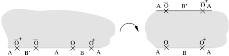
Figure 5: Conformal mapping of the infinite half plane with $\omega={L\over\pi}\ln({z\over L})$ to the strip.

References

- [1] J. L. Cardy, Nucl. Phys. B 324, 581 (1989).
- [2] I. Affleck and A. W. W. Ludwig, J. Phys. A 27, 5375 (1994).
- [3] I. Affleck, in Correlation effects in low-dimensional electron systems, Vol. 118 of Springer Series in Solid-State Sciences, edited by A. Okiji and N. Kawakami (Springer Verlag, Berlin, 1994), pp. 82–95.
- [4] H. Schulz, J. Phys. C 18, 581 (1985).
- [5] F. Alcaraz, M. Barber, M. Batchelor, R. Baxter, and G. Quispel, J. Phys. A 20, 6397 (1987).
- [6] E. K. Sklyanin, J. Phys. A 21, 2375 (1988).
- [7] L. Mezincescu, R. I. Nepomechie, and V. Rittenberg, Phys. Lett. A 147, 70 (1990).
- [8] P. W. Anderson, Phys. Rev. Lett. 18, 1049 (1967).
- [9] S. Qin, M. Fabrizio, and L. Yu, Phys. Rev. B 54, R9643 (1996).
- [10] P. Nozières and C. T. de Dominicis, Phys. Rev. 178, 1097 (1969).
- [11] K. D. Schotte and U. Schotte, Phys. Rev. 182, 479 (1969).
- [12] I. Affleck, preprint (1996), hep-th/9611064.
- [13] S. Tomonaga, Prog. Theor. Phys. 5, 544 (1950).
- [14] J. M. Luttinger, J. Math. Phys. 4, 1154 (1963).
- [15] A. Luther and I. Peschel, Phys. Rev. B 12, 3908 (1975).
- [16] H. Frahm and V. E. Korepin, Phys. Rev. B 42, 10533 (1990).
- [17] H. Frahm and V. E. Korepin, Phys. Rev. B 43, 5653 (1991).
- [18] N. Kawakami and S.-K. Yang, J. Phys. Condens. Matter 3, 5983 (1991).
- [19] H. Asakawa and M. Suzuki, J. Phys. A 29, 225 (1996).
- [20] F. H. L. Eßler, J. Phys. A 29, 6183 (1996).
- [21] A. Kapustin and S. Skorik, J. Phys. A 29, 1629 (1996).
- [22] H.-Q. Zhou, Phys. Rev. B 54, 41 (1996).
- [23] F. H. L. Eßler, V. E. Korepin, and K. Schoutens, Nucl. Phys. B 384, 431 (1992).
- [24] C. N. Yang, Phys. Rev. Lett. 63, 2144 (1989).
- [25] S. Skorik and H. Saleur, J. Phys. A 28, 6605 (1995).
- [26] Y. Wang and J. Voit, Phys. Rev. Lett. 77, 4934 (1996).
- [27] F. H. L. Eßler and H. Frahm, to be published.
- [28] M. Shiroishi and M. Wadati, J. Phys. Soc. Japan 66, 1 (1997).
- [29] T. Deguchi and R. Yue, 1996, preprint.
- [30] F. Woynarovich, J. Phys. A 22, 4243 (1989).
- [31] S. Fujimoto and N. Kawakami, Phys. Rev. B 54, 5784 (1996).
- [32] Y. Wang, J. Voit, and F.-C. Pu, Phys. Rev. B 54, 8491 (1996).