Global symmetries of quantum Hall systems: lattice description

Abstract

I analyze non-local symmetries of finite-size Euclidean 3D lattice Chern-Simons models in the presence of an external magnetic field and non-zero average current. It is shown that under very general assumptions the particle-vortex duality interchanges the total Euclidean magnetic flux ${\bf\Phi}/2\pi$ and the total current ${\bf I}$ in a given direction, while the flux attachment transformation increases the flux in a given direction by the corresponding component of the current, ${\bf\Phi}/2\pi\rightarrow{\bf\Phi}/2\pi+2{\bf I}$, independently of the disorder. In the language of $2\!+\!1$ dimensional models, appropriate for describing quantum Hall systems, these transformations are equivalent to the symmetries of the phase diagram known as the Correspondence Laws, and the non-linear current–voltage mapping between mutually dual points, recently observed near the quantum Hall liquid–insulator transitions.

]

Introduction

Beginning with the analysis of the Ising model by Kramers and Wannier[1] in early forties, the particle–vortex duality found extensive use in physics. However, duality had been always considered as a kind of “theoretical” symmetry, whose manifestations are limited to the critical region and generally are very hard to observe. This is one of the reasons why the experiments[2, 3, 4] observing a precise duality between the adjacent quantum Hall phases came as a total surprise. The agreement with the apparently simple theory[5] combining the duality transformation and the random phase approximation (RPA) went far beyond the original expectations of the authors. In fact, experimentally[2] the duality was shown to relate the entire set of non-linear $I$–$V$ curves in a surprisingly wide region of temperatures, gate voltages and magnetic fields, indicating that the dynamics on the two sides of the transitions must be very similar. This is in spite of the fact that theoretically, according to the very same duality mapping, the elementary particle excitations at the two sides of the transition, fermions and fractionally charged vortex-like quasiparticles, are very different! Even more surprising are the experimental indications of duality between the two phases in the metal–insulator phase transitions[6, 7], apparently observed in silicon MOSFETs in the absence of a magnetic field, where the conventional theory of localization predicted no phase transition at all.

The fractionally charged quasiparticles were introduced by Laughlin[8] as excitations on top of the highly-correlated state now known as the Laughlin liquid; these objects were used to explain the observed fractional values of the Hall conductance. Unfortunately, the wavefunction description does not easily reveal the order parameter associated with different phases and it could not be used to study the phase transitions between the plateaus. The interpretation of the peculiar off-diagonal long-range order inherent to Laughlin’s wavefunction as the condensation of the composite particles was proposed[9] by Girvin and MacDonald. These ideas were later developed[10] by Zhang, Hansson and Kivelson, who derived the Chern-Simons-Landau-Ginzburg (CSLG) theory[11] directly from the microscopic Hamiltonian. The symmetries of the ground-state wavefunction now became apparent as the (approximate) non-trivial symmetries of the model itself. These symmetries impose many important constraints on the allowed phase transitions and were used[5] by Kivelson, Lee and Zhang (KLZ) to construct the Global Phase Diagram of the quantum Hall system.

Despite all the success of the CSLG theory and its excellent experimental confirmation[12, 13, 14, 15, 16, 2, 3, 4], some questions still remain unanswered. The most important of these questions is why does so simple a model work so well. The original KLZ calculations were done only within the RPA approximation, and the universality of the scalar field correlators was conjectured rather than derived. Indeed, the quasiparticles have different charges and even their fractional statistics differ, and one would think that the global universality in this picture is not likely to happen. For example, calculations[17, 18], perturbative in the Chern-Simons coupling, indicate that this additional gauge coupling is at least a marginally relevant perturbation to the model of free bosons. Similar calculation[19], performed without the $1/N$ expansion suppressing the effect of gauge degrees of freedom, demonstrated that the Chern-Simons gauge interaction is actually a relevant perturbation to the scalar field fixed point; this interaction leads to a first-order phase transition in the regime where perturbation theory applies.

A formal symmetry-based approach to the problem of the quantum Hall phase transitions was initiated[20, 21] by Lutken and Ross, and later further developed[22, 23] to apply for the beta-function flows. The idea was to find all the consequences of the observed SL(2,Z) symmetry group without specifying how this symmetry is achieved. In the spirit of the two-parameter scaling model of the quantum Hall effect[24, 25], it was postulated that the partition function and the scaling beta-function for the complexified conductance $\Sigma=\Sigma_{xy}+i\Sigma_{xx}$ of the system, are invariant under the elements of SL(2,Z) and can depend on $\Sigma$ only as “quasi-holomorphic” functions. This assumption, together with the known behavior in the limits of weak and strong coupling, severely restricts the phase diagram and the possible functional form of beta-function. Unfortunately, so far nobody has managed to complete this program and find the critical exponents in the vicinity of the critical point relying on the symmetry considerations, alone.

As an alternative to the conventional perturbative approach, S.-C. Zhang and the author attempted[26] to understand the universality of the quantum Hall transitions using the lattice x-y model coupled with the Chern-Simons gauge field, which comes naturally as the strong-coupling regime of the CSLG model. They constructed the exact duality and flux attachment transformations on the lattice and proved that the Chern-Simons field is the most relevant interaction in this problem and, modulo the irrelevant higher-order in momenta terms, the phase transitions in different Chern-Simons models with the coefficients related by these transformations must be in the same universality class. Fradkin and Kivelson[27], in addition to the model similar to that of Ref.[26], considered a model where the gauge-field polarization operator acquires an additional $T$-symmetric, linear in momenta part. The corresponding dimensionless coupling constant, combined with the usual Chern-Simons coefficient, forms a complex-valued parameter $z$ which transforms according to a subgroup of the modular group SL(2,Z). In particular, there are infinitely many fixed points that remain invariant under certain elements of this group. It was proposed that corresponding values of the parameter $z$ must coincide with the critical points of the quantum Hall system. Once again, symmetry requires the conductivity in these critical points to have certain (generally different for different fixed points) universal values.

The major advantage of Chern-Simons x-y models is that they allow to treat the gauge fields, apparently the most relevant part of the interaction, non-perturbatively, considering all other interactions as less relevant. On the other hand, the lattice models considered so far did not have precisely the same symmetries as the continuum CSLG model derived[10] directly from the microscopic Hamiltonian of electrons. Specifically, the lattice models[26, 27] have the exact rotational symmetry (or relativistic one after the Wick rotation) while the scalar field in Refs.[10, 5] is non-relativistic. In addition, none of the lattice models was constructed carefully enough to allow the finite-size scaling analysis in the presence of external magnetic field, current or charge density.

The goal of this work is to construct a lattice Chern-Simons model as a regularization of the continuum CSLG model in the limit of strong short-range electron-electron repulsion, at the same time keeping track of the long-distance properties of the model. I show that the required model is exactly the Chern-Simons x-y model, extended to include a non-zero flux of external magnetic field and a non-zero average current density. Even though this model is written in rotationally (relativistically) covariant form, the Lorentz symmetry is broken by the external current (the last component of which corresponds to the charge density) and the external magnetic field, so that both by construction and by its symmetry the model represents a quantum Hall system. It is shown that under very general assumptions, in addition to transformations of the Chern-Simons coupling[26], the duality interchanges the total magnetic flux ${\bf\Phi}/2\pi$ and the total current ${\bf I}$ in a given direction, while the flux attachment transformation increases the total magnetic flux in a given direction by the corresponding component of the total electrical current, ${\bf\Phi}/2\pi\rightarrow{\bf\Phi}/2\pi+2{\bf I}$.

The derived transformations, after being reinterpreted in terms of the $2\!+\!1$ dimensional systems, are equivalent to the symmetries of the phase diagram known as Correspondence Laws[5], as well as the nonlinear current–voltage mapping between mutually dual points, recently observed[2] near the quantum Hall liquid–insulator transitions. Even though the exact symmetries of the phase diagram can be derived within other approaches, like, for example, the 2D CFT formulation[28], only within the CS x-y model one can understand the non-linear transport relationships as well. Unlike the previously studied continuum models where the problems of renormalization are unavoidable, here the current–voltage mapping is exact and is an immediate consequence of the duality regardless of the specific form of the gauge and scalar-field coupling. Moreover, these symmetries hold in the presence of arbitrary potential and magnetic disorder, which remain unchanged by either the duality or the flux attachment (up to a short-radius formfactor coming from the different size of the quasiparticles in different representations). This implies that the derived results will hold even if the disorder, marginal by the power counting, turns out to be a relevant perturbation.

The Section I introduces the lattice Chern-Simons x-y model in an external gauge field as the lattice regularization of the phase part of the CSLG model after integration over the density fluctuations. The infrared behavior of this model is controlled by defining it on a torus using the magnetic translation group. The duality and flux attachment transformations of the lattice model are discussed in Sections II and III respectively. The application of derived results to the real-time quantum Hall systems, including the derivation of the Correspondence Laws[5] and the current–voltage duality, are presented in Sec. IV.

Before ending this Introduction, I would like to remark that there have been a great number of publications on the problem of phase transitions and the duality in the quantum Hall system, and it would be impossible to list even all the approaches here. An excellent summary of plausible interpretations of the experiment[2] and the key difficulties associated with these interpretations was recently given[29] by Shimshoni, Sondhi and Shahar.

I Definition of the model

A Lattice and continuum Chern-Simons models

The Euclidean partition function of the Chern-Simons x-y model with an external field can be written as

$${\cal Z}=\prod\int d{\bf a}\,d\theta\,e^{-i{\cal S}_{\theta}(\theta,{\bf a}+{\bf A})-i{\cal S}_{a}({\bf a})},$$ (1)

where the gauge part

$$i{\cal S}_{a}={1\over 2}\int{d^{3}k\over(2\pi)^{3}}{\bf a}_{-{\bf k}}{\cal K}({\bf k}){\bf a}_{\bf k},$$ (2)

and scalar part

$$i{\cal S}_{\theta}=-{1\over T}\sum\cos(\nabla\theta-{\bf a}-{\bf A})$$ (3)

of the action depend on the phases $\theta$ defined at every vertex of the three-dimensional cubic lattice, while the Chern-Simons gauge field ${\bf a}$ and external gauge field ${\bf A}$ live on the links. As usual for lattice gauge theories, the value of ${\bf A}$ on the link can be interpreted as the integral of the physical gauge field along this link

$${\bf A}_{n,n+\hat{\mu}}=\int_{{\bf r}_{n}}^{{\bf r}_{n+\hat{\mu}}}{\bf A}_{\mu}({\bf x})d{\bf x}^{\mu};$$

for notational convenience, in this paper the contour sums of gauge quantities are denoted as the continuum integrals along the appropriate contours. Similarly, the flux of the magnetic field through some area, a sum over plaquettes in the discrete lattice model, will be denoted as the continuum surface integral of the field over this area. These notations were chosen for the sake of readability of the paper. The Reader interested in the details of the lattice definition of the Chern-Simons term is directed to Ref. [26].

The dynamics of the field ${\bf a}$ is determined by the transverse gauge kernel ${\cal K}({\bf k})$. The most general rotationally-invariant form of this kernel can be written as the sum of $T$-antisymmetric and $T$-symmetric parts

$${\cal K}^{\mu\nu}({\bf k})=f(k)e^{\mu\nu\rho}{\bf P}_{\rho}+g(k)\left(P^{2}\delta^{\mu\nu}-{\bf P}_{\mu}{\bf P}_{\nu}\right),$$ (4)

depending on the lattice momentum ${\bf P}_{\mu}=2\sin(k_{\mu}/2)$. It is the small-momentum behavior of the functions $f$ and $g$ that determines the properties of the model, as has been shown in Refs.[26, 27]. Specifically, the usual Chern-Simons model can be defined by the condition

$$\lim\limits_{k\rightarrow 0}f(k)={f_{0}\over 2\pi}={1\over 2\pi\,\alpha}\quad{\rm and}\quad\lim\limits_{k\rightarrow 0}kg(k)=0.$$ (5)

The generalization of this standard form considered by Fradkin and Kivelson[27], has both limits finite,

$$\lim\limits_{k\rightarrow 0}f(k)={f_{0}\over 2\pi}\quad{\rm and}\quad\lim\limits_{k\rightarrow 0}kg(k)={g_{0}\over 2\pi}.$$ (6)

Unlike the usual Chern-Simons model, the model with such a kernel has self-dual fixed points; they were associated[27] with the fixed points of the quantum Hall phase transitions.

As defined, the partition function (1) is symmetric with respect to simultaneous change of the sign of all components of the fields $\nabla\theta$, ${\bf a}$ and ${\bf A}$; since the phase gradient is associated with the current, both the external magnetic field and the current are reversed,

$${\bf j}\rightarrow-{\bf j},\quad{\bf a}\rightarrow-{\bf a},\quad{\bf A}\rightarrow-{\bf A}.$$ (7)

This trivial symmetry preserves the handedness of the coordinate system, and therefore does not change the sign of the pseudoscalar $\alpha$. One can also change the handedness of the coordinate system, simultaneously reversing the sign of $\alpha$ and all pseudovectors like the magnetic field. In terms of the global flux of the total magnetic field ${\bf\Phi}=\int\nabla\!\times\!\left({\bf A}+{\bf a}\right)\,d{\bf s}$, this transformation can be written as

$${\bf\Phi}=-{\bf\Phi}^{\prime},$$ (8)

while polar vectors, (for example, the particle current density ${\bf j}$), remain unchanged.

At first glance, the lattice model (1) seems to be only vaguely related to the quantum Hall problem. As defined, this model treats all coordinates evenly, unlike the continuum CSLG model[10, 11] with the action

$$S=S_{a}+S_{\varphi}=\int dtd^{2}x\,{\cal L}_{a}+\int dtd^{2}x\,{\cal L}_{\varphi},$$ (9)

which has a similar gauge part ${\cal L}_{a}={e^{\mu\nu\rho}a_{\mu}\partial_{\nu}a_{\rho}}/(4\pi\alpha)$, but an explicitly non-relativistic scalar part

$${\cal L}_{\varphi} = \varphi^{{\dagger}}\left(i\partial_{t}-a_{t}-{A_{t}}\right)\varphi$$ (11)

$$-{1\over 2m_{e}}\left|\left(i\vec{\nabla}+\vec{a}+\vec{A}\right)\varphi\right|^{2}-{V\over 2}(\varphi^{{\dagger}}\varphi-\overline{\rho})^{2}$$

defined in terms of the wavefunction $\varphi=\sqrt{\rho}\exp{i\theta}$ of the bosonic condensate, where $\theta$ and $\rho$ are the corresponding microscopic phase and density.

Note, however, that even in the absence of the gauge fields, the lattice model (1) represents only the phase sector of the continuum model (9); any such model should have a linear-spectrum mode as long as there is a finite phase stiffness generating the propagation velocity $v$. Formally, the relativistically-symmetric form of the phase action can be obtained[30] by integrating away the fluctuations of the density $\rho=\varphi^{\dagger}\varphi$ near its average value $\overline{\rho}$, which leads to the Lagrangian

$${\cal L}_{\theta}={k\over 2}\left[{1\over v^{2}}(\partial_{t}\theta+a_{t}+A_{t})^{2}-\left(\vec{\nabla}\theta+\vec{a}+\vec{A}\right)^{2}\right]$$ (12)

dependent on the phase $\theta$ only. Here $k=\overline{\rho}/m_{e}$ and $v^{2}=\overline{\rho}V/m_{e}$ are the effective stiffness and velocity of the phase excitations calculated with frozen gauge fields; certainly, these values should be understood as bare values of the parameters.

Even after the density integration, the “relativistic” symmetry of the model (12) is not exact: it is broken by the external gauge field ${\bf A}$ which reflects the presence of a uniform magnetic field and both scalar and magnetic disorder. After the Wick rotation $t\rightarrow i\tau$, $A_{t}\rightarrow-iA_{z}$, the normal component of the magnetic field $B=\partial_{x}{\bf A}_{y}-\partial_{y}{\bf A}_{x}$ becomes the last component of the Euclidean magnetic field $B_{z}=B$, while the components of the lateral electric field

$$\vec{E}=-\vec{\nabla}A_{t}-\partial_{t}\vec{\bf A}$$

correspond to the remaining components $B^{j}=i\varepsilon^{ji}E_{i};$ clearly, the analytic continuation from the imaginary values of external fields is needed to relate the results of the two approaches. Similarly, physical charge density $\rho$ and the current density $\vec{\hbox{\it\j}}$ determine the three components of the Euclidean current density ${\bf j}^{\mu}$ whose average values can be obtained from the partition function (1) by differentiating with respect to the components of the Euclidean gauge field,

$$\langle{\bf j}^{\mu}\rangle=-{1\over i}{\delta\log Z\over\delta A_{\mu}}.$$ (13)

This implies the correspondence ${\bf j}^{\mu}\rightarrow(\rho,\,i\vec{\hbox{\it\j}})$; the spatial components of the Euclidean current acquire imaginary value and, once again, the analytic continuation must accompany the Wick rotation.

B Magnetic translations and periodic boundary conditions

By going from the continuum Lagrangian (12) to the lattice action (3) we regularized all possible ultra-violet divergences. To finish the definition of the model, it is now necessary to regularize its infrared behavior. This can be done by defining the model on a closed surface like a torus. Let us imagine the finite-size system of interest as a unit cell of an infinite lattice, where all gauge-invariant quantities are perfectly periodic. On the other hand, a gauge field cannot obey the periodic boundary conditions in any two directions if it has a non-zero magnetic flux in the perpendicular direction. The exact periodicity in such a system can be established using the operators of magnetic translation, defined as the combination of the ordinary translation and the special gauge transformation restoring the original form of the Hamiltonian.

As an example, consider a simplified version of lattice model (3) where the Chern-Simons field has been frozen,

$$i{\cal S}_{\rm min}=-{1\over T}\sum_{\bf r}\cos\left(\nabla\theta-{\bf A}\right),$$ (14)

which is just the three-dimensional x-y model minimally coupled to an external magnetic field. Even though the vector potential changes under the gauge transformation

$$\theta\rightarrow\theta+f,\quad{\bf A}\rightarrow{\bf A}+\nabla f,$$ (15)

the magnetic field ${\bf B}=\nabla\!\times\!{\bf A}$ and all physical observables remain invariant.

Similarly, a displacement by a period ${\bf L}_{\mu}$ in a given direction $\mu=x$, $y$ or $z$ changes the vector potential by the increment defined as ${\hbox to8.8889pt{\hfill\hbox{$\cdot$}\hfill}\hskip-8.8889pt\hbox{$\triangle$}}_{\mu}{\bf A}({\bf r})\equiv{\bf A}({\bf r}+{\bf L}_{\mu})-{\bf A}({\bf r})$. Since the gauge-invariant magnetic field $\nabla\!\times\!{\bf A}$ is periodic by assumption, its increment ${\hbox to8.8889pt{\hfill\hbox{$\cdot$}\hfill}\hskip-8.8889pt\hbox{$\triangle$}}_{\mu}$ vanishes, ${\hbox to8.8889pt{\hfill\hbox{$\cdot$}\hfill}\hskip-8.8889pt\hbox{$\triangle$}}_{\mu}(\nabla\!\times\!{\bf A})=\nabla\!\times\!{\hbox to8.8889pt{\hfill\hbox{$\cdot$}\hfill}\hskip-8.8889pt\hbox{$\triangle$}}_{\mu}{\bf A}=0$, so that the increment ${\hbox to8.8889pt{\hfill\hbox{$\cdot$}\hfill}\hskip-8.8889pt\hbox{$\triangle$}}_{\mu}$ of the vector potential ${\bf A}$ can be expressed as a gradient,

$${\hbox to8.8889pt{\hfill\hbox{$\cdot$}\hfill}\hskip-8.8889pt\hbox{$\triangle$}}_{\mu}{\bf A}({\bf r})=\nabla F_{\mu}({\bf r}).$$ (16)

The newly-defined scalar function generates the gauge transformation (15) with $f=-F_{\mu}$, which exactly restores the original form of the model. Therefore, even though the exact form of the model (14) is changed by both the translations and gauge transformations, their combination preserves each term of this model. Such combination of a translation and a gauge transformation define the “magnetic translation” $\hat{T}({\bf L}_{\mu})$. As in the case of uniform magnetic field, the magnetic translations $\hat{T}({\bf L}_{\mu})$ and $\hat{T}({\bf L}_{\nu})$ commute with each other only if the magnetic flux through the area ${\bf L}_{\mu}\!\times\!{\bf L}_{\nu}$ is equal to an integer number of flux quanta $\phi_{0}=hc/e$.

Let us utilize the magnetic translation symmetry to specify the periodic boundary conditions for our lattice system in the region $0\leq{\bf r}_{i}<{\bf L}_{i}$. The angle $\theta$ in the point $(x,y,{\bf L}_{z})$ outside the boundaries of this region must be replaced by the appropriately corrected angle in $(x,y,0)$ using the symmetry with respect to magnetic translations

$$\theta(x,y,{\bf L}_{z})-F_{z}(x,y,{\bf L}_{z})\equiv\theta(x,y,0);$$ (17)

similar patching conditions must be defined for the two remaining “outer” surfaces of the system. The expression (17) contains only the part of the function $F_{z}(x,y,{\bf L}_{z})$ at the “top” face $z={\bf L}_{z}$ of the this region of interest; similarly only the values $F_{x}({\bf L}_{x},y,z)$ and $F_{y}(x,{\bf L}_{y},z)$ of two other patching functions at their corresponding “upper” faces are relevant. Each of these in-plane values obeys a simpler two-dimensional equation

$${\hbox to8.8889pt{\hfill\hbox{$\cdot$}\hfill}\hskip-8.8889pt\hbox{$\triangle$}}_{\mu}{\bf A}_{\perp}=\nabla_{\perp}F_{\mu}$$ (18)

instead of Eq. (16), where the index “$\perp$” denotes the part of the vector orthogonal to the axis “$\mu$”. In the following it is assumed that the patching functions $F_{\mu}$ are functions of only two variables in the corresponding plane ${\bf r}_{\mu}={\bf L}_{\mu}$, $\mu=x$, $y$, or $z$.

Generally, under the gauge transformation (15) the fields ${\bf A}$ at the opposite faces of the system transform differently, so that the values of the increments ${\hbox to8.8889pt{\hfill\hbox{$\cdot$}\hfill}\hskip-8.8889pt\hbox{$\triangle$}}_{\mu}{\bf A}_{\perp}$ change. To preserve the condition (18), we need to adjust the patching functions, $F_{\mu}\rightarrow F_{\mu}+{\hbox to8.8889pt{\hfill\hbox{$\cdot$}\hfill}\hskip-8.8889pt\hbox{$\triangle$}}_{\mu}f$. This transformation rule, along with the original definition (18), can be satisfied by defining

$$F_{\mu}({\bf r}_{\perp})=\int\limits_{\rm BCDA}{\bf A}({\bf r})\cdot d{\bf r}+{\rm Const},$$ (19)

where the integration is performed along the three-part contour starting in the point ${\rm B}\equiv{\bf r}_{\perp}+{\bf L}$ and ending in ${\rm A}\equiv{\bf r}_{\perp}$ as shown in FIG. 1: two congruent lines BC and DA along the opposite faces of the system, connected by a fixed contour CD entering both faces in equivalent points. An arbitrary gauge-invariant constant introduced in Eq. (19) accounts for the freedom of uniformly “twisting” the boundary conditions for $\theta$; it is also the freedom of choosing the configuration of the fixed segment CD of the “back flow” contour BCDA.

FIG. 1.: The coupling of the gauge field with the current line $\rm AB$ is made gauge-invariant by introducing the surface patching term (19), equivalent to integration along the contour $\rm BCDA$. The line $\rm BC$ is the image of $\rm AD$ after translation by the period ${\bf{}L}_{z}$.

C 2D example

Before advancing any further the analysis of the three-dimensional problem, let us analyze a simpler two-dimensional Villain x-y model

$$i{\cal S}_{\rm V}={1\over 2T}\sum_{\bf r}{\left(\nabla\theta-{\bf A}-2\pi{\bf m}\right)^{2}}$$ (20)

in external magnetic field. In expression (20) the angles $\theta$ are defined in the vertices of two-dimensional square lattice, the vector potential of the external magnetic field is defined at the links, as well as the additional integer-valued field ${\bf m}$ which restores the periodicity broken after changing the cosines of the original x-y model for parabolas in the Villain approximation.

At every link the summation in appropriate component of ${\bf m}$ is independent of anything else and can be transformed with the Poisson summation formula,

$${1\over 2T}\left(\nabla\theta-{\bf A}-2\pi{\bf m}\right)^{2}\longrightarrow{T{\bf j}^{2}\over 2}-i{\bf j}\cdot\left(\nabla\theta-{\bf A}\right).$$ (21)

replacing the summation over ${\bf m}$ by the summation over new independent integer-valued variables ${\bf j}$ also defined at every link of the lattice.

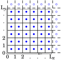
FIG. 2.: Solid lines denote the definition region of the 2D Villain x-y model, while the filled circles show the corresponding vertices of the dual lattice. Region outside the thin solid contour represent the images of the points after translation(s).

Normally, the term with the gradient of $\theta$ in Eq. (21) can be integrated by parts, $-i{\bf j}\cdot\nabla\theta\rightarrow i\theta\nabla\cdot{\bf j}$, so that the subsequent integration in $\theta$ renders the conservation law

$$\nabla\cdot{\bf j}=0,$$ (22)

which, given the form of its coupling to the gauge field, allows to identify ${\bf j}$ as the conserved current. In the finite system, however, the phases $\theta$ in equivalent points across the boundary of the system are related by the patching equations (17), and the integration by parts generates additional boundary terms

$$i{\cal S}_{\rm surf}=-i\int_{0}^{{\bf L}_{y}}{\bf j}^{x}\cdot F_{x}(y)dy-i\int_{0}^{{\bf L}_{y}}{\bf j}^{y}\cdot F_{y}(x)dx,$$ (23)

where the patching functions $F_{i}$ are related to the increments of the gauge field across the system,

$${\hbox to8.8889pt{\hfill\hbox{$\cdot$}\hfill}\hskip-8.8889pt\hbox{$\triangle$}}_{x}{\bf A}_{y}=\nabla_{y}F_{x}(y),\qquad{\hbox to8.8889pt{\hfill\hbox{$\cdot$}\hfill}\hskip-8.8889pt\hbox{$\triangle$}}_{y}{\bf A}_{x}=\nabla_{x}F_{y}(x).$$ (24)

As before, these equations define the functions $F_{x}$ and $F_{y}$ up to arbitrary additive constants.

The term with the square of the current ${\bf j}$ in Eq. (21) can be split by the Hubbard-Stratonovich transformation,

$${T{\bf j}^{2}\over 2}\rightarrow i{\bf b}{\bf j}+{{\bf b}^{2}\over 2T},$$

where ${\bf b}$ is the new auxiliary field defined at the links of the lattice. Although this field couples with the current like an additional gauge field, the integration in ${\bf b}$ is performed over all possible values including different gauges; this field is not a gauge field. By construction, the field ${\bf b}$ is defined only within the period of the system and, therefore, it satisfies periodic boundary conditions and does not introduce any non-trivial total magnetic flux.

Now let us resolve the conservation law (22) by introducing an integer-valued scalar field $h$ associated with the vertices of the dual lattice ${\bf j}^{\mu}=\epsilon^{\mu\nu}\nabla_{\nu}h\equiv\widetilde{\nabla}^{\mu}h$. This definition implies that the increments of the additional field $h$ across the system are related to the total currents in perpendicular directions,

$${\hbox to8.8889pt{\hfill\hbox{$\cdot$}\hfill}\hskip-8.8889pt\hbox{$\triangle$}}_{x}h=-I_{y}\quad{\rm and}\quad{\hbox to8.8889pt{\hfill\hbox{$\cdot$}\hfill}\hskip-8.8889pt\hbox{$\triangle$}}_{y}h=I_{x};$$ (25)

because of the periodicity and the current conservation these increments remain constant along the edges.

At this point the effective action can be written as

$$i{\cal S}_{\rm V}=\int\left\{{{\bf b}^{2}\over 2T}+i({\bf b}+{\bf A})\widetilde{\nabla}h\right\}dS+i{\cal S}_{\rm surf},$$ (26)

where the surface patching term ${\cal S}_{\rm surf}$ is given by Eq. (23). To arrive at the dual representation of the model we need to integrate the gauge coupling by parts, using the identity

$${\bf A}_{\mu}\epsilon^{\mu\nu}\nabla_{\nu}h\equiv{\bf A}\!\times\!\nabla h=h\,\nabla\!\times\!{\bf A}-\nabla\!\times({\bf A}h).$$

The last term of this expression results in a contour integral along the edge of the system, which can be split into vertical and horizontal parts,

$$-\oint h\,{\bf A}\,d{\bf l}=\int_{0}^{{\bf L}_{x}}\!\!{\hbox to8.8889pt{\hfill\hbox{$\cdot$}\hfill}\hskip-8.8889pt\hbox{$\triangle$}}_{y}({\bf A}_{x}h)dx-\!\int_{0}^{{\bf L}_{y}}\!\!{\hbox to8.8889pt{\hfill\hbox{$\cdot$}\hfill}\hskip-8.8889pt\hbox{$\triangle$}}_{x}({\bf A}_{y}h)dy.$$ (27)

With the increments of fields ${\bf A}$ and $h$ known, we can transform the increments of their products using the expression

$${\hbox to8.8889pt{\hfill\hbox{$\cdot$}\hfill}\hskip-8.8889pt\hbox{$\triangle$}}_{x}(fg)=f({\bf L}_{x},y){\hbox to8.8889pt{\hfill\hbox{$\cdot$}\hfill}\hskip-8.8889pt\hbox{$\triangle$}}_{x}g+g({\bf L}_{x},y){\hbox to8.8889pt{\hfill\hbox{$\cdot$}\hfill}\hskip-8.8889pt\hbox{$\triangle$}}_{x}f-{\hbox to8.8889pt{\hfill\hbox{$\cdot$}\hfill}\hskip-8.8889pt\hbox{$\triangle$}}_{x}f{\hbox to8.8889pt{\hfill\hbox{$\cdot$}\hfill}\hskip-8.8889pt\hbox{$\triangle$}}_{x}g,$$ (28)

so that the contour integral (27) takes the form

$$-\oint h\,{\bf A}\,d{\bf l} = \int_{0}^{{\bf L}_{x}}\!\left(\nabla_{x}F_{y}\,h+I_{x}{\bf A}_{x}-I_{x}\nabla_{x}F_{y}\right)dx$$ (29)

$$- \int_{0}^{{\bf L}_{y}}\!\left(\nabla_{y}F_{x}\,h-I_{y}{\bf A}_{y}+I_{y}\nabla_{y}F_{x}\right)dy.$$ (30)

The first term in each of these integrals can be integrated by parts, with the integrated part once again evaluated using Eq. (28). With the expression for the total flux of the magnetic field, $\Phi={\hbox to8.8889pt{\hfill\hbox{$\cdot$}\hfill}\hskip-8.8889pt\hbox{$\triangle$}}_{y}F_{x}-{\hbox to8.8889pt{\hfill\hbox{$\cdot$}\hfill}\hskip-8.8889pt\hbox{$\triangle$}}_{x}F_{y}$, following immediately from the Stokes formula and the definition (24), we obtain

$$-\oint h\,{\bf A}\,d{\bf l} = \int_{0}^{{\bf L}_{y}}\!{\bf j}_{x}F_{x}dy+\int_{0}^{{\bf L}_{x}}\!{\bf j}_{y}F_{y}dx-h({\bf L}_{x},{\bf L}_{y})\Phi$$ (33)

$$+I_{x}\left\{\int_{0}^{{\bf L}_{x}}\!\!{\bf A}_{x}dx+\Phi-F_{x}({\bf L}_{y})\right\}$$

$$+I_{y}\left\{\int_{0}^{{\bf L}_{y}}\!\!{\bf A}_{y}dx-\Phi-F_{y}({\bf L}_{x})\right\}.$$

The first two terms cancel exactly with the edge patching term (23), while the remaining terms can be eliminated by properly defining the so far arbitrary additive constants for the scalar field $h$ and the patching functions $F_{i}$. Specifically, defining $h({\bf L}_{x},{\bf L}_{y})=0$,

$$F_{x}({\bf L}_{y})=\int_{0}^{{\bf L}_{x}}A_{x}(x,{\bf L}_{y})dx+\Phi$$

and

$$F_{y}({\bf L}_{x})=\int_{0}^{{\bf L}_{y}}A_{y}({\bf L}_{x},y)dy-\Phi,$$

eliminates the last two terms in Eq. (33), so that the performed integration by parts can be written simply as

$$\int A\times\!\nabla h\,dS\,+\,{\cal S}_{\rm surf}=\int h\,\nabla\times{\bf A}\,d{\bf s}.$$

Although the described procedure works generally for any gauge field ${\bf A}$, we had to be careful to separate the contribution from the Hubbard-Stratonovich field ${\bf b}$: the gauge-fixing terms cannot depend on this field. The field ${\bf b}$ is periodic and the equivalent series of transformations is much simpler, immediately leading to

$$-\oint h\,{\bf b}\,d{\bf l}=I_{x}\!\int_{0}^{{\bf L}_{x}}\!{\bf b}_{x}dx+I_{y}\!\int_{0}^{{\bf L}_{y}}\!{\bf b}_{y}dy$$ (34)

instead of Eq. (33). It is convenient to use the potential representation ${\bf b}_{i}=\nabla_{i}f+\epsilon^{ij}\nabla_{j}g$ with the condition that the normal derivatives of both potentials vanish at the boundary, $\partial g/\partial n=\partial f/\partial n=0$. Then it follows from the periodicity

$$\int{\bf b}^{2}\,dS=\int(\nabla f)^{2}+(\nabla g)^{2}\,dx\,dy,$$

and the transformed action (26) can be written as

$$i{\cal S}_{\rm V}=\!\int\!\!\left\{{(\nabla g)^{2}\over 2T}+ih\,(\nabla\!\times\!{\bf A}-\nabla^{2}g)\right\}dS+\!\int\!\!{(\nabla f)^{2}\over 2T}dS$$

$$+i(I_{x}+I_{y})\,f({\bf L}_{x},{\bf L}_{y})-iI_{x}\,f(0,{\bf L}_{y})-iI_{y}\,f({\bf L}_{x},0),$$

with the free terms in the last line resulting from the line integrals (34). It is clear that the two potentials $f$ and $g$ in this action are completely independent of each other. The summation over integer $h$ only fixes the vortex charges $\upsilon=\nabla\!\times\!{\bf A}-\nabla^{2}g$ to integer values modulo $2\pi$. Since the field ${\bf b}$ is single-valued, it does not contribute any additional flux and the total vorticity must be exactly equal to the total flux of the external magnetic field.

Furthermore, the term $\int(\nabla g)^{2}dS/2T$ precisely equals to the Coulomb energy associated with the vortex charges in the uniform background. This can be proven by introducing an auxiliary field $\phi$,

$${(\nabla g)^{2}\over 2T}\rightarrow{T(\nabla\phi)^{2}\over 2}+i\nabla\phi\nabla g\rightarrow{T(\nabla\phi)^{2}\over 2}-i\phi\nabla^{2}g$$

$$={T(\nabla\phi)^{2}\over 2}-2\pi i\phi\upsilon+i\phi{\nabla\!\times\!{\bf A}},$$

where the integrated part vanished because of the boundary condition $\partial g/\partial n=0$.

The considered transverse part of the dual action is independent of the lateral currents $I_{x}$, $I_{y}$ encoded in the discontinuity of the boundary condition (25) for the field $h$. These currents act as the only sources of the scalar potential $f$. The energy of the equivalent Coulomb problem, quadratic in these currents, provides the only current-dependent contribution to the free energy; this contribution is obviously non-critical.

II Duality in three dimensions

Now let us resume the analysis of the Chern-Simons gauge model in three dimensions. The major steps include: (i) Start with the canonical form (1) of the model and rewrite it in terms of conserved integer-valued current ${\bf j}$ and auxiliary field ${\bf b}$. (ii) Resolve the current conservation law by introducing an additional integer-valued field ${\bf m}$, ${\bf j}=\nabla\!\times\!{\bf m}$, integrate the current coupling by parts and prove that, as a result of summation in ${\bf m}$, the flux of the total gauge field through every plaquette is an integer, identified with the dual conserved current. Up to this point all transformations will be done exactly for any form of the original x-y model. (iii) In the Villain approximation, integrate over the longitudinal part of the field ${\bf b}$ to allow treating of its remaining part as a gauge field. (iv) Finally, resolve the constraint on the original Chern-Simons gauge field by yet another Hubbard-Stratonovich transformation, and express the result in the canonical form (1).

i Introduce the integer-valued current:

Before introducing the surface patching terms for the model (1), it is convenient to transform its scalar part (3) to the equivalent current representation

$$i{\cal S}_{\theta}=i\sum{\bf j}\cdot\left(\nabla\theta\!-\!{\bf a}\!-\!{\bf A}\!-\!{\bf b}\right)-\sum{\cos{\bf b}\over T},$$ (35)

where the original form (3) is restored after the summation over all integer ${\bf j}$ and subsequent integration over the auxiliary field ${\bf b}$ at every link. As in the two-dimensional example, the integration over the phases $\theta$ imposes the conservation constraint $\nabla\cdot{\bf j}=0$, so that ${\bf j}$ can be identified as the integer-valued current.

Assuming the kernel ${\cal K}$ is transverse (i.e. $({\cal K}{\bf a})$ gauge-invariant,) it is easy to find the required form

$$i{\cal S}_{\rm surf}=i\sum_{i}\int_{S_{i}}F_{i}\,\left({\bf j}-{1\over 2}{\cal K}{\bf a}\right)\cdot d{\bf s}$$ (36)

of the surface terms required to fix the gauge-invariance in the finite system. Here $F_{i}$ are the patching functions for the sum of two gauge fields ${\bf a}_{\rm tot}={\bf a}+{\bf A}$ as defined in Appendix A, and the integration areas ${\rm S}_{i}$ are the three visible faces of the cube as shown in FIG. 3. Since the auxiliary field ${\bf b}$ is single-valued, it creates no total magnetic flux through the system and there are no boundary patching terms associated with this field.

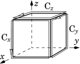
FIG. 3.: The integration areas ${\rm S}_{i}$ in the surface patching terms (36) are limited by the contours ${\rm C}_{i}$, $i=x$, $y$, $z$.

The surface patching terms (36) make the model gauge-invariant, but they also eliminate the integration over the constant part of the fluctuating gauge field ${\bf a}$ along with the resulting mean-field constraint

$$\int{\cal K}{\bf a}\,d\Omega=-i\int{\bf j}\,d\Omega.$$ (37)

For the model with purely Chern-Simons gauge kernel (5), Eq. (37) is the condition on the average flux of the associated magnetic field $\langle\nabla\!\times\!{\bf a}\rangle=2\pi\alpha\,\langle{\bf j}\rangle$. This constraint allows us to associate the model (1) with the continuum CSLG model (9) and ultimately with the real quantum Hall systems; therefore the constraint (37) needs to be imposed on the original model (1) by integration over an additional uniform auxiliary field.

ii Resolve the current conservation:

By analogy with the two-dimensional problem, we can resolve the lattice current-conservation constraint $\nabla\!\cdot{\bf j}=0$ by introducing an auxiliary field ${\bf m}$,

$${\bf j}=\nabla\!\times{\bf m}.$$ (38)

There is, however, an important difference with the two-dimensional case: in 3D the gauge freedom associated with the solution of Eq. (38) is much more broad. Simultaneously, in generic gauge ${\bf m}$ is not an integer-valued field, and even the existence of the integer-valued solution is not immediately obvious.

Let us choose the gauge $m_{z}=0$, then it is easy to check that the sums

$$m_{x}(x,y,z) = \int_{0}^{z}\!\!j_{y}(x,y,\zeta)d\zeta-\int_{0}^{x}j_{z}(\xi,y,0)d\xi,$$ (39)

$$m_{y}(x,y,z) = -\int_{0}^{z}\!\!j_{x}(x,y,\zeta)d\zeta$$ (40)

satisfy Eq. (38); by construction this solution is integer-valued. Now we may introduce the patching functions $G_{i}$ associated with the integer-valued gauge field ${\bf m}$. Explicit calculation shows that both $G_{x}=0$ and $G_{y}=0$ up to an integer constant, and

$$\partial_{x}G_{z}(x,y)=\int_{0}^{{\bf L}_{z}}j_{y}dz,\qquad\partial_{y}G_{z}(x,y)=-\int_{0}^{{\bf L}_{z}}j_{y}dz;$$

these equations have a solution since the curl

$$\partial_{y}(\partial_{x}G_{z})-\partial_{x}(\partial_{y}G_{z}) = \int_{0}^{{\bf L}_{z}}\!\left(\partial_{x}j_{x}+\partial_{y}j_{y}\right)\,dz$$

$$= -\int_{0}^{{\bf L}_{z}}\!\partial_{z}j_{z}\,dz=0$$

vanishes. According to Eq. (A1), the complete current-dependent coupling can be integrated by parts as

$$\int\!\nabla\!\times\!{\bf m}\cdot({\bf b}+{\bf a}_{\rm tot})\,d\Omega+{\cal S}_{\rm surf}=\int\!{\bf m}\cdot\nabla\!\times\!({\bf b}+{\bf a}_{\rm tot})\,d\Omega$$ (42)

$$+\sum_{i=x,y,z}I_{i}\int_{0}^{{\bf L}_{i}}\!{\bf b}_{i}\,dx_{i}+\int_{S_{z}}\!\!G_{z}\left[\nabla\times\!({\bf b}+{\bf a}_{\rm tot})\right]_{z}\,d{\bf s},$$

where ${\bf a}_{\rm tot}={\bf a}+{\bf A}$. Independent summations over $m_{x}$ and $m_{y}$ restrict the $x$- and $y$- components of the field

$${\bf v}={1\over 2\pi}\nabla\times\!({\bf b}+{\bf a}_{\rm tot})$$ (43)

to integer values. This field is a total curl, and consequently it is conserved, $\nabla\!\cdot\!{\bf v}=0$. Therefore, the differences $\partial_{z}{\bf v}_{z}$ of the $z$-component of this field at adjoining links are also integer-valued. Finally, the summation of the patching surface term at the surface $S_{z}$ over the values of the function $G_{z}$ restricts the values of ${\bf v}_{z}$ at this surface to integer values, completing the proof that all components of the field ${\bf v}$ can take only integer values. This conserved field ${\bf v}$ will be identified as the dual integer-valued current.

Up to this point all transformations were exact and very general, valid for virtually any imaginable form of the lattice gauge model. Eq. (43) relates the lines of the dual current to the flux lines of the combined magnetic field $\nabla\!\times\!({\bf A}+{\bf a}+{\bf b})$, so that the total dual current through the system

$$\widetilde{\bf I}=\int{\bf v}\,d{\bf s}={1\over 2\pi}\int\nabla\!\times\!({\bf A}+{\bf a})\,d{\bf s}={{\bf\Phi}\over 2\pi}$$ (44)

in any given direction is precisely equal to the total number of flux quanta ${\bf\Phi}/2\pi$ of the combined magnetic field in this direction (the contribution of the periodic auxiliary field ${\bf b}$ vanishes after the surface integration). This universal relationship between the total current and the total magnetic flux in mutually dual models is one of the central results of this work. Previously, a similar result, relating the flux of the magnetic field with the number of vortices, was obtained by Lee and Fisher[31, 32], in an approximate lattice duality involving a “softening” of the integer constraint on the total number of vortices.

iii Integrate away the scalar potential:

The goal of the subsequent steps is to rewrite the dual action in a form possibly close to that of the original action (3). This can be done only approximately, ignoring some terms irrelevant in the RG sense. In particular, the integration over the auxiliary gauge field ${\bf b}$ will be done only in the Villain approximation, leaving out the non-linear corrections. With this in mind, the result of the summation of the combined action (2), (35) over the integer-valued current ${\bf j}$ can be written as

$$i{\cal S}_{\rm cs} \rightarrow \int{{\bf b}^{2}\over 2T}d\Omega+{1\over 2}\int{\bf a}{\cal K}{\bf a}\,d\Omega$$ (46)

$$+i\sum_{\mu=x,y,z}I_{\mu}\int_{0}^{{\bf L}_{\mu}}\!{\bf b}_{\mu}\,dx_{\mu}+(\text{surface terms}).$$

Here the field ${\bf a}$ is a solution of the equation

$$\nabla\!\times\!{\bf a}=2\pi{\bf v}-\nabla\!\times\!({\bf b}+{\bf A}),$$ (47)

while the Hubbard-Stratonovich field ${\bf b}$ and the conserved dual integer-valued current ${\bf v}$ with given total flux $\int{\bf v}\,d{\bf s}={\bf\Phi}/2\pi$ through the sample are independent variables. The presence of surface terms ensure that the expression (46) does not depend on the particular gauge chosen for the solution ${\bf a}$ of Eq. (47).

Following the two-dimensional example, we can eliminate the integrals of ${\bf b}$ in the second line of Eq. (46) by writing ${\bf b}=\nabla\phi+\nabla\!\times\!{\bf g}=\nabla\phi+{\bf b}^{\prime}$, with the tangential part of the second term vanishing everywhere at the surface of the system. Then the integration over the field $\phi$ yields a non-critical quadratic in the currents ${\bf I}_{i}$ contribution to the free energy, proportional to the energy of the Coulomb interaction of the charges $\pm{\bf I}_{i}$ set in the corners of the cube in FIG. 3 and their mirror images.

Now the constraint on the boundary values of the field ${\bf b}^{\prime}$ can be removed by adding the appropriate surface patching terms rendering the expression gauge-independent; this is possible because the surface terms evaluate to zero with the original boundary condition of vanishing tangential components of the field ${\bf b}^{\prime}$. The gauge fields ${\bf a}$ and ${\bf b}^{\prime}$ enter Eq. (47) only in the combination ${\bf a}^{\prime}={\bf a}+{\bf b}^{\prime}$; integrating away their difference we obtain the combined gauge coupling[26]

$${({\bf b}^{\prime})^{2}\over 2T}+{1\over 2}{\bf a}{\cal K}{\bf a}\rightarrow{1\over 2}{\bf a}^{\prime}{\cal K}^{\prime}{\bf a}^{\prime},\qquad{\cal K}^{\prime}=\left(T+{\cal K}^{-1}\right)^{-1},$$

where the field ${\bf a}^{\prime}$ satisfies the equation

$$\nabla\!\times\!{\bf a}^{\prime}=2\pi{\bf v}-\nabla\!\times\!{\bf A},$$

and all inverse matrices must be evaluated in the transverse gauge $\nabla\cdot{\bf a}=0$.

iv Introduce new auxiliary field:

Finally, we need to express the coupling ${\bf a}^{\prime}{\cal K}^{\prime}{\bf a}^{\prime}$ as a path integral over an additional auxiliary field ${\bf c}$. With the appropriate surface patching integrals implicit, this can be done by the Hubbard-Stratonovich transformation

$${1\over 2}{\bf a}^{\prime}{\cal K}^{\prime}{\bf a}^{\prime}\rightarrow i{\bf a}^{\prime}\cdot\nabla\!\times\!{\bf c}+{1\over 2}(\nabla\!\times\!{\bf c}){{\cal K}^{\prime}}^{-1}(\nabla\!\times\!{\bf c}),$$ (48)

where the additional constraint on the total flux of the auxiliary field through the system

$$\int\nabla\!\times\!{\bf c}\,d{\bf s}=-i\int{\cal K}^{\prime}{\bf a}^{\prime}\,d{\bf s}=-{\bf I}$$ (49)

is mandated by the degeneracy of the gauge kernel ${\cal K}^{\prime}$ at zero momentum due to the presence of the surface patching terms. Indeed, the Hubbard-Stratonovich transformation (48) can be interpreted as the addition in the exponent

$${\bf a}^{\prime}{\cal K}^{\prime}{\bf a}^{\prime}\rightarrow{\bf a}^{\prime}{\cal K}^{\prime}{\bf a}^{\prime}+\left(\nabla\!\times\!{\bf c}+i{\cal K}^{\prime}{\bf a}^{\prime}\right){{\cal K}^{\prime}}^{-1}\left(\nabla\!\times\!{\bf c}+i{\cal K}^{\prime}{\bf a}^{\prime}\right),$$

with the subsequent integration in ${\bf a}^{\prime}$; the condition (49) is required for the inverse operator to be meaningful.

With the help of Eq. (47), the total Lagrangian becomes

$$i\widetilde{\cal L}_{\rm cs}=i{\bf c}\cdot(2\pi{\bf v}-\nabla\!\times\!{\bf A})+{(\nabla\!\times\!{\bf c}){{\cal K}^{\prime}}^{-1}(\nabla\!\times\!{\bf c})\over 2}.$$ (50)

After defining the dual gauge field

$$\nabla\!\times\!\tilde{\bf a}=2\pi\nabla\!\times\!{\bf c}-2\pi i\,{\cal K}^{\prime}{\bf A},$$

we can write the Lagrangian of the system in the form

$$i\widetilde{\cal L}_{cs}={{\bf A}{\cal K}^{\prime}{\bf A}\over 2}+i{\bf v}\left(\tilde{\bf a}-2\pi\,(i\nabla\times)^{-1}{\cal K}^{\prime}\,{\bf A}\right)+{\tilde{\bf a}\,\widetilde{\cal K}^{\prime}\,\tilde{\bf a}\over 2},$$ (51)

where the dual gauge kernel

$$\widetilde{\cal K}={{\bf P}\times{{\cal K}^{\prime}}^{-1}\times{\bf P}\over(2\pi)^{2}}={TP^{2}\over(2\pi)^{2}}-{{\bf P}\times{\cal K}^{-1}\times{\bf P}\over(2\pi)^{2}},$$

and the total flux $\widetilde{\Phi}$ of the gauge fields coupled to the dual current ${\bf v}$ is determined by the original particle current,

$$\widetilde{\Phi}=\int\left(\nabla\!\times\!\tilde{\bf a}+2\pi i{\cal K}^{\prime}A\right)\,d{\bf s}=-2\pi{\bf I}$$ (52)

as immediately follows from Eq. (49) and the definition of the dual gauge field $\tilde{\bf a}$. It is easy to see that the second duality transformation restores the form of the model up to the trivial symmetry (7).

In the limit of small momenta or slow-varying external field ${\bf A}$, and assuming the original gauge kernel (6) has purely Chern-Simons form (5), the important part of the dual model can be written as

$$\widetilde{\cal L}_{\rm cs}\sim{\bf v}\left(\tilde{\bf a}+{1\over\alpha}\,{\bf A}\right)+{\alpha\over 4\pi}({\tilde{\bf a}\partial\tilde{\bf a}})+i{T\over 4\pi^{2}}(\nabla\!\times\!\tilde{\bf a})^{2},$$ (53)

indicating that, up to irrelevant difference in the quasiparticle’s size, the dual model is the Chern-Simons Villain x-y model with the excitations of electric charge $1/\alpha$, statistics $-1/\alpha$, and the dimensionful lattice temperature[26, 27] $\tilde{T}=T/\alpha^{2}$.

The global conditions on the total dual flux (52) and current (44) restore the mean-field constraint (37) for the dual model only if the gauge kernel of the original model has purely Chern-Simons form (5). Indeed,

$$\int\!\nabla\!\times\!\tilde{\bf a}\,d{\bf s} \stackrel{{\scriptstyle(\ref{eq:3d-dual-flux})}}{{=}} \widetilde{\bf\Phi}-{{\bf\Phi}_{A}\over\alpha}=-2\pi{\bf I}-{{\bf\Phi}_{A}\over\alpha}$$

$$= -{2\pi\over\alpha}\left(\alpha{\bf I}+{{\bf\Phi}_{A}\over 2\pi}\right)=-{1\over\alpha}{\bf\Phi}\stackrel{{\scriptstyle(\ref{eq:total-dual-current})}}{{=}}-{2\pi\over\alpha}\tilde{\bf I},$$

where ${\bf\Phi}_{A}$ denotes the total flux of the external magnetic field. It is this property that shows that the chosen definition of the gauge coupling in finite systems is natural and corresponds to the expected behavior for the model describing quantum Hall systems. The relationship of the considered class of models to the quantum Hall effect will be discussed more specifically in Sec. IV.

Unfortunately, it is not clear how to perform the transition between Eqns. (50) and (51) for the generalized form of the Chern-Simons coupling (4), which is supposed[27] to describe the even-denominator (metallic) fixed points of the quantum Hall system. In this case the background charge density fluctuations in Eq. (50) cannot be self-consistently traded for the modified magnetic field in Eq. (51), indicating that additional entities like the “magnetic” charges[27] are needed. At this time, it is not clear what physical meaning can be attributed to such objects.

III Flux attachment transformation

In addition to the duality, the continuum Chern-Simons models have another important symmetry, the periodicity, or the symmetry under the flux attachment transformation. In this section I show that the lattice version of this transformation is exact and, in addition to modifying the Chern-Simons coefficient[26], changes the magnetic flux ${\bf\Phi}$ by the amount proportional to the global current ${\bf I}$.

Let us fix a configuration of integer-valued conserved current ${\bf j}$ and define the related gauge field ${\bf c}_{\bf j}$ as a solution of the equation $\nabla\!\times\!{\bf c}_{\bf j}=4\pi{\bf j}$. In a system where the current lines never cross the boundary, the coupling

$$X={1\over 2}\int{\bf c}_{\bf j}\,{\bf j}\,d\Omega+\text{surface terms}$$ (54)

is always an integer times $2\pi$. Because of the surface patching terms, this coupling is always an integer times $2\pi$, independent of the gauge chosen for the field ${\bf c}_{\bf j}$. Indeed, for the current lines that do cross the boundary, the surface terms can be interpreted as the “back flow” currents, as shown in FIG. 1, and the statement for the closed current lines apply.

We would like to rewrite the coupling (54) as a path integral over a dynamical variable ${\bf c}$ instead,

$$X=\int\left[{\bf c}\!\cdot\!{\bf j}-{({\bf c}\partial{\bf c})\over 8\pi}\right]\,d\Omega+\text{surface terms},$$ (55)

but the explicit calculation shows that this expression does not contain an integration variable needed to fix the total flux of the field ${\bf c}$. To set this flux correctly, we need to add the term

$$\lambda_{\mu}\left({\bf j}-{\nabla\!\times\!{\bf c}\over 4\pi}\right)_{\mu}$$

with integration over the components of the uniform auxiliary field $\lambda_{\mu}$. This is equivalent to restoring the integration over the uniform part of the field ${\bf c}$ removed by the surface patching terms; the whole expression still remains gauge-invariant. With the addition of this constraint, the integration in Eq. (55) yields exactly the self-coupling (54).

Because it is always an integer multiple of $2\pi$, the expression (55) can be introduced as an additional phase to the partition function (1) without changing its value. As a result, the full partition function contains a minimal coupling of the integer-valued current ${\bf j}$ to the sum of two fields ${\bf a}^{\prime}={\bf a}+{\bf c}$ with their respective gauge kernels ${\cal K}^{\mu\nu}$ and ${\cal{}K}_{0}^{\mu\nu}=ie^{\mu\nu\rho}\nabla_{\rho}/(4\pi)$. After integrating away[26] the difference of these fields, the resulting model has the gauge-invariant coupling to the field ${\bf a}^{\prime}$ with the gauge kernel

$${\cal K}^{\prime}=\left({\cal K}^{-1}+{\cal K}_{0}^{-1}\right)^{-1}$$ (56)

with the Chern-Simons coefficient $\alpha^{\prime}=\alpha+2$. Since both fields ${\bf a}$ and ${\bf c}$ were constrained to have a fixed total magnetic flux, the combined field ${\bf a}^{\prime}$ has the magnetic flux

$${\bf\Phi}^{\prime}={\bf\Phi}+4\pi{\bf I}$$ (57)

in every direction. Clearly, the total magnetic flux increased by twice the number of the particle’s world lines propagating through the system in the same direction, while the total particle current ${\bf I}$ remains unchanged.

Similarly to the duality, the flux attachment transformation preserves the mean-field constraint (37) for the models with purely Chern-Simons gauge kernel (5). Therefore, imposing such a constraint once for the initial model immediately sets it for the whole hierarchy of models generated by the duality and flux attachment transformations, in agreement with our expectations for the models describing plateau transitions in quantum Hall systems.

IV Correspondence Laws

The hierarchy transformations of the CS x-y model change the microscopic dimensionless charge $\alpha$ defined through the gauge coupling kernel (4), and, more importantly, they also modify the global parameters, the Euclidean current and the magnetic flux, in a universal fashion. It turns out that these global transformations are formally equivalent to the Correspondence Laws, suggested[5] and confirmed experimentally[15, 16, 2, 3, 4], as the symmetries of the quantum Hall phase diagram. This analogy can be seen in the real-time representation, which requires treating the charge-density $\rho$ and the lateral current $\vec{\hbox{\it\j}}$ separately.

i Symmetries of the phase diagram.

The Wick rotation transforms the third component ${\bf j}_{z}$ of the Euclidean current into the charge density $\rho$, while the corresponding component of the total magnetic field $B_{\rm tot}=\nabla\!\times\!({\bf a}+{\bf A})$ is transformed to the component of the magnetic field normal to the two-dimensional plane of motion of particles. It is convenient to express the global transformations of the x-y model in terms of the bosonic filling fraction $\nu_{\rm b}=2\pi\langle\rho\rangle/\langle B_{\rm tot}\rangle$:

reflection (8): $$\nu_{\rm b}\rightarrow-\nu_{\rm b},$$ (58)

duality (44), (52): $$\nu_{\rm b}\rightarrow-\nu_{\rm b}^{-1},$$ (59)

flux attachment (57): $$\nu_{\rm b}^{-1}\rightarrow\nu_{\rm b}^{-1}+2,$$ (60)

which are formally equivalent to the Correspondence Laws[5] for fermions. Indeed, by attaching a flux quantum to every boson, we can convert it to a fermion in a modified magnetic field, their filling fractions related through the identity $1/\nu_{\rm b}=1/\nu_{\rm f}-1$. Then each of the basic transformations for fermions become equivalent to a combination of transformations (58)–(60), as explicitly shown in Table I.

Transformation	Fermions	Bosons
Landau level addition	$\nu_{\rm f}\rightarrow\nu_{\rm f}+1$	$\nu_{\rm b}\rightarrow-\nu_{\rm b}^{-1}-2$
flux attachment	$\nu_{\rm f}^{-1}\rightarrow\nu_{\rm f}^{-1}+2$	$\nu_{\rm b}^{-1}\rightarrow\nu_{\rm b}^{-1}+2$
particle-hole symmetry	$\nu_{\rm f}\rightarrow 1-\nu_{\rm f}$	$\nu_{\rm b}\rightarrow\nu_{\rm b}^{-1}$

TABLE I.: The Laws of Correspondence in terms of Fermionic $\nu_{\rm f}$ and Bosonic $\nu_{\rm b}$ filling fractions related by the identity $1/\nu_{\rm b}=1/\nu_{\rm f}-1$.

Experimentally[2, 3, 4], the duality symmetry was observed for the transitions between the quantum Hall liquid and insulator. Specifically, the 2DEG demonstrates reciprocal longitudinal resistance and the mirror symmetry of non-linear $I$–$V$ curves in the points at the phase diagram, related by the expression

$$\left(\alpha-{\nu}^{-1}\right)\left(\alpha-{\tilde{\nu}}^{-1}\right)=1,$$ (61)

where $\alpha$ is an odd integer value of the quantized Hall resistance in the corresponding plateaus, measured in the units of $h/e^{2}$, and $\nu=2\pi\rho/B$ is the measured filling fraction of the electrons, which is varied across the transition. In terms of the “bosonic” filling fractions $\nu_{\rm b}=(\alpha-{\nu}^{-1})^{-1}$, this relationship can be written simply as $\nu_{\rm b}\,\tilde{\nu}_{\rm b}=1$, which is equivalent to the combination of the duality (59) with the reflection (58). Note, that the measured value of the filling fraction $\nu_{c}$ in the transition point is close but not exactly equal to the theoretical value $\nu^{\ast}_{c}=(\alpha+1)^{-1}$, implying that the quasiparticles are not in one-to-one correspondence with the original electrons. A partial mixing of the opposite spin states, not included in the theoretical model, provides a qualitative explanation for this discrepancy.

ii Symmetries of transport coefficients.

The remaining two components of the Euclidean current ${\bf j}=(\rho,i\vec{\hbox{\it\j}})$ originate from the lateral current $\vec{\hbox{\it\j}}$ of the $2\!+\!1$ dimensional system, while the in-plane Euclidean magnetic field is generated by the electric field

$${{\bf B}_{x}}\rightarrow i{E_{y}},\quad{{\bf B}_{y}}\rightarrow-i{E_{x}}.$$ (62)

The rotation by $\pi/2$ is needed to transform the components of the axial vector ${\bf B}$ into the polar vector ${\vec{E}}$; the inversion of the handedness changes both the sign of ${\bf B}$ and the sign of the rotation angle, so that the relation (62) remains valid. Unlike that for the usual charge density and magnetic field, the Wick rotation of spatial components involve the complex phase $i=e^{i\pi/2}$, indicating that the analytic continuation in the values of these fields is needed. Any singularity encountered during this procedure would invalidate the current–voltage mapping. This is certainly related to the fact that the presence of the electric field $\vec{E}$ and the current density $\vec{\hbox{\it\j}}$ may involve dissipation. However, this mapping is valid in all orders of the perturbation expansion in powers of the electric field $\vec{E}$; the actual region of validity of this procedure is determined by the convergence of the perturbation series, as well as the presence and the relative importance of non-perturbative terms.

The duality interchanges the components of the current density with the appropriate components of the rotated electric field. In terms of physical electric field and current density, the duality relationship can be written as

$$\left({\tilde{E}_{x,y}\over 2\pi\,\tilde{\hbox{\it\j}}_{y,x}}\pm\alpha\right)\left({E_{x,y}\over 2\pi\,\hbox{{\it j\/}}_{y,x}}\pm\alpha\right)=1,$$ (63)

where the first (second) indices correspond to top (bottom) signs. In the linear regime the substitution ${\vec{E}}=\hat{\rho}\,\vec{\hbox{\it\j}}$ and $\vec{\tilde{E}}=\hat{\tilde{\rho}\,}\vec{\tilde{\hbox{\it\j}}}$ shows that the equation (63) is equivalent to the inversion of the bosonic resistivity tensor

$$\hat{\rho}_{b}\equiv{{\hat{\sigma}}_{b}}^{-1}=\hat{\tilde{\sigma}}_{b}={\hat{\tilde{\rho}\,}\!}_{b}^{-1}$$ (64)

between the mutually dual points. Here the bosonic resistivity tensors are related to the usual resistivity tensors, measured in the units of $hc/e=2\pi\,\hbar c/e$, by the relationship

$$\hat{\rho}_{b}=\hat{\rho}-\alpha\left(\begin{array}[c]{cc}0&1\\ -1&0\end{array}\right).$$ (65)

As pointed out in Ref.[29], Eq. (64) corresponds to the inversion of the longitudinal resistivity $\tilde{\rho}_{xx}=1/\rho_{xx}$ observed in experiment[2] as long as the Hall resistivity remains equal to its quantized value $\rho_{xy}=\alpha$, or, equivalently,

$$\sigma_{xy}^{2}+\sigma_{xx}^{2}=\alpha^{-1}\sigma_{xy}.$$

This statement, known as the Semicircle Law, is associated with the presence of disorder, and is known to hold exactly for two-component systems[33, 34].

iii Universality of phase transitions.

Perturbatively[17, 18, 19], the universality of phase transitions in Chern-Simons models does not seem to be a probable outcome. However, the universality was proven[26] for the transitions in the clean CS x-y model where the “relativistic” symmetry is not broken by external magnetic field or total charge density. In the absence of these fields the independent parameter $\nu$ is absent, and the hierarchy mapping between the vicinities of phase transitions at different values of $\alpha$ is complete. The exact universality class depends on whether the given fractional value of the Chern-Simons coefficient originates from bosons or fermions, but it is not likely to correspond to that of any phase transition experimentally observed in quantum Hall systems.

In the extended CS x-y model (1), where both the external magnetic field and the charge density can be present, there are at least two independent parameters that characterize the state of the equilibrium system: the filling fraction $\nu$ and the Chern-Simons coefficient $\alpha$. Transforming both of them at each step, it is impossible to construct a mapping between two quantum Hall states of electrons ($\alpha=1$). Even though the proof of the universality[26] remains formally valid, in the presence of non-zero filling fraction the universality applies not to the original electrons, but to vortices, particles with the transformed Chern-Simons coefficient, at the dual filling fraction. In the original formulation of the hierarchy theory[5], this problem is resolved by making an assumption about the independence of the bosonic current-current correlation function of the Chern-Simons coefficient. So far, even though an ample experimental evidence confirming this non-trivial assumption is available, a rigorous theoretical proof, or even an effective model that would display this behavior, is missing.

Any possible scenario explaining this puzzle must include the disorder. For example, if the disorder-associated scattering turns out strong enough to screen the correlations associated with the Chern-Simons interaction at large distances, the effective disorder-averaged model will be independent of the Chern-Simons coefficient. Since both the duality and the flux attachment preserve the shape of the disorder potential, it is conceivable that the disorder-averaged model would nevertheless inherit the original hierarchy symmetries, at least in some range of parameters. This point of view is supported by the bulk of experimental data[12, 13, 14, 15, 16, 2, 3, 4], which indicates that the fractional and integer quantum Hall transitions are in the same universality class, and their vicinities are at least approximately related by the Correspondence Laws.

Conclusion

The Chern-Simons x-y model with external fields considered here was constructed as a lattice regularization of the CSLG model. Even though this model is written in rotationally (relativistically) covariant form (1)–(3), the non-zero charge-current density and external magnetic and electric fields break the Lorentz symmetry in exactly the same way as it is broken in the original continuum model. In addition, the studied model demonstrates the same non-local symmetries as the CSLG model—only at the lattice these symmetries can be formulated as exact statements, without the limitations of the RPA approximation used in the continuum model.

Unfortunately, neither model clears the issue of the observed universality of phase transition. Note, however, that both the duality and the flux attachment transformation remain exact in the Chern-Simons x-y model even in the presence of disorder; the latter is merely carried from one representation to another without any significant change of the statistical properties. It is easy to check[35] that in the replicated version of this model the disorder averaging commutes with the duality transformation. This gives a hope that there exists an effective description of diffusion in this strongly-interacting system, independent of the Chern-Simons coupling and, therefore, symmetric with respect to hierarchy transformations.

Apart from this issue of universality, the analyzed CS x-y model appears to be a perfect candidate for providing an effective description of the quantum Hall phase transitions. In this second-quantized model the non-local duality and flux attachment transformations can be performed exactly. These transformations are expressed in terms of system-averaged charge and current density and also the electric and magnetic fields; they generate the experimentally observed global symmetries of the phase diagram known as the Correspondence Laws[5], and the nonlinear current–voltage mapping between mutually dual points[2]. The global nature of the transformed parameters imply that they are not subject to renormalization. Moreover, the derived duality relationship is so robust and insensitive to particular details of both interaction and disorder, that the immediately following $I$–$V$ reflection symmetry could be viewed as a signature of the duality of this kind.

In this context, a similar and so far unexplained current–voltage symmetry observed[6, 7] in the conductor–insulator transition in silicon MOSFETS at zero magnetic field appears especially suggesting. Certainly, there remains a more mundane possibility that the observed symmetry is a mere consequence of the universal critical scaling.

A Hermiticity of the Chern-Simons coupling

Here I derive the conditions of Hermiticity

$$\int(a\partial b)d\Omega \!-\! \sum_{i}\int_{S_{i}}G_{i}\nabla\times{\bf b}\cdot d{\bf s}$$ (A1)

$$= \int(b\partial a)d\Omega-\sum_{i}\int_{S_{i}}F_{i}\nabla\times{\bf a}\cdot d{\bf s}$$ (A2)

for the gauge-invariant Chern-Simons coupling in finite systems, with the patching functions $G_{i}$ and $F_{i}$ defined (up to the additive constants specified below) by the expressions

$$\nabla G_{i}={\hbox to8.8889pt{\hfill\hbox{$\cdot$}\hfill}\hskip-8.8889pt\hbox{$\triangle$}}_{i}{\bf a},\qquad\nabla F_{i}={\hbox to8.8889pt{\hfill\hbox{$\cdot$}\hfill}\hskip-8.8889pt\hbox{$\triangle$}}_{i}{\bf b}$$ (A3)

Consider the difference of two volume integrals

$$J=\int{\bf a}\cdot\nabla\times{\bf b}\;d\Omega - \int{\bf b}\cdot\nabla\times{\bf a}\;d\Omega$$

$$=\int\nabla\cdot({\bf b}\times{\bf a})\;d\Omega = \oint{\bf b}\times{\bf a}\cdot d{\bf s}$$

transformed to the integral over the full outer surface of the system, which can be split into the contributions from three pairs of parallel faces,

$$J = \sum_{i=\{x,y,z\}}J_{i},$$ (A4)

$$J_{i} = \int_{S_{i}}\nabla F_{i}\times\left({\bf a}-{1\over 2}\nabla G_{i}\right)\cdot d{\bf s}$$ (A6)

$$-\int_{S_{i}}\nabla G_{i}\times\left({\bf b}-{1\over 2}\nabla F_{i}\right)\cdot d{\bf s}.$$

In each term the integration is limited to the front $S_{x}$, right $S_{y}$ or top $S_{z}$ sides of the system as shown in FIG. 3, and the patching functions (A3) were used to simplify the increments of the gauge fields across the system. Each of these six integrals can be further transformed using the vector identity

$$\nabla F\times{\bf a}=\nabla\times\left({\bf a}\,F\right)-F\,\nabla\times{\bf a}$$

into the sum of the contour integral and the surface integral

$$\int\limits_{S}\!\nabla F\times\left(\!\!{\bf a}-{\nabla G\over 2}\!\right)d{\bf s}=\!\oint\limits_{C}\!F\left(\!\!{\bf a}-{\nabla G\over 2}\!\right)\!\cdot d{\bf l}-\!\int\limits_{S}\!F\nabla\!\times\!{\bf a}\cdot d{\bf s}.$$

In every case the surface integral cancels with one of the surface patching terms in $J$. Therefore, the Chern-Simons coupling with appropriate edge patching terms is a Hermitian operator as specified by Eq. (A1) if and only if the sum of all line integrals

$$L=\sum_{i}\oint_{C_{i}}F_{i}\left({\bf a}-{1\over 2}G_{i}\right)\cdot d{\bf l}-\biggl{[}\begin{array}[c]{c}a\leftrightarrow b\\ G\leftrightarrow F\end{array}\biggr{]}$$ (A7)

vanishes.

The closed line integrals in Eq. (A7) can be simplified by grouping together the contributions of the parallel parts of each contour, and once again using the patching functions for the differences of the gauge fields

$$L = e^{xyz}\int_{0}^{{\bf L}_{y}}dy\biggl{\{}F_{z}\left(a_{y}-{1\over 2}G_{z,y}\right)$$ (A12)

$$-\left(F_{z}-{\hbox to8.8889pt{\hfill\hbox{$\cdot$}\hfill}\hskip-8.8889pt\hbox{$\triangle$}}_{x}F_{z}\right)\left(a_{y}-{1\over 2}G_{z,y}-G_{x,y}+{1\over 2}{\hbox to8.8889pt{\hfill\hbox{$\cdot$}\hfill}\hskip-8.8889pt\hbox{$\triangle$}}_{x}G_{z,y}\right)\biggr{\}}$$

$$-\biggl{[}\begin{array}[c]{c}a\leftrightarrow b\\ G\leftrightarrow F\end{array}\biggr{]}.$$

Here we imply the summation over all permutations of the coordinates, $G_{z,y}\equiv\partial_{y}G_{z}$, and the functions are evaluated at the segment $({\bf L}_{x},y,{\bf L}_{z})$ or its equivalents generated by cyclic permutations of the coordinates. It is convenient to use the symmetries of the expression (A12) and write symbolically

$$L = \sum_{12}\int_{0}^{{\bf L}_{y}}\biggl{\{}\left(F_{z}-{\hbox to8.8889pt{\hfill\hbox{$\cdot$}\hfill}\hskip-8.8889pt\hbox{$\triangle$}}_{x}F_{z}\right)\left(G_{x,y}-{1\over 2}{\hbox to8.8889pt{\hfill\hbox{$\cdot$}\hfill}\hskip-8.8889pt\hbox{$\triangle$}}_{x}G_{z,y}\right)$$ (A14)

$$+{\hbox to8.8889pt{\hfill\hbox{$\cdot$}\hfill}\hskip-8.8889pt\hbox{$\triangle$}}_{x}F_{z}\left(a_{y}-{1\over 2}G_{z,y}-G_{x,y}\right)\biggr{\}}dy,$$

implying the summation over six permutations of the coordinates and two additional permutations of the gauge fields $a$ and $b$ with their corresponding parity factors. This way one does not need to write all terms explicitly in order to simplify the expression (A14). For example, the integral

$$\sum_{12}\int F_{z}G_{x,y}\,dy = {1\over 2}\sum_{12}\int\left(F_{z}G_{x,y}+G_{x}F_{z,y}\right)\,dy$$

$$= {1\over 2}\sum_{12}\left.(F_{z}G_{x})\right|_{0}^{{\bf L}_{y}}\equiv{1\over 2}\sum_{12}{\hbox to8.8889pt{\hfill\hbox{$\cdot$}\hfill}\hskip-8.8889pt\hbox{$\triangle$}}_{y}(F_{z}G_{x})$$

$$\hskip-28.45274pt=\hskip 28.45274pt \hskip-28.45274pt{1\over 2}\sum_{12}{\hbox to8.8889pt{\hfill\hbox{$\cdot$}\hfill}\hskip-8.8889pt\hbox{$\triangle$}}_{y}F_{z}\,G_{x}+F_{z}\,{\hbox to8.8889pt{\hfill\hbox{$\cdot$}\hfill}\hskip-8.8889pt\hbox{$\triangle$}}_{y}G_{x}-{\hbox to8.8889pt{\hfill\hbox{$\cdot$}\hfill}\hskip-8.8889pt\hbox{$\triangle$}}_{y}F_{z}\,{\hbox to8.8889pt{\hfill\hbox{$\cdot$}\hfill}\hskip-8.8889pt\hbox{$\triangle$}}_{y}G_{x}.$$

Some additional simplification can be achieved by using the expression for the total flux of the gauge field

$${\hbox to8.8889pt{\hfill\hbox{$\cdot$}\hfill}\hskip-8.8889pt\hbox{$\triangle$}}_{y}F_{x}-{\hbox to8.8889pt{\hfill\hbox{$\cdot$}\hfill}\hskip-8.8889pt\hbox{$\triangle$}}_{x}F_{y}=\oint_{C_{z}}{\bf a}\cdot d{\bf l}={\bf\Phi}_{z}^{a}$$

in $z$-direction, and similar expressions for other components of ${\bf a}$ and the field ${\bf b}$. After some rather tedious but straightforward algebra the expression (A14) simplifies to

$$L=\sum_{6}{\bf\Phi}_{y}^{a}\left(F_{y}-\int_{0}^{{\bf L}_{y}}b_{y}dy+{1\over 2}{\bf\Phi}_{z}^{b}-{1\over 2}{\bf\Phi}_{x}^{b}\right).$$ (A15)

The function $F_{y}$ in this expression is evaluated at the vertex $({\bf L}_{x},{\bf L}_{y},{\bf L}_{z})$ and the integration in $y$ is performed along the line $x={\bf L}_{x}$, $z={\bf L}_{z}$.

With the help of Eq. (A15) we can fix the so far arbitrary constants in the definition (A3) of the surface patching functions $F_{i}$ and $G_{i}$. Specifically, by defining

$$F_{y}({\bf L}_{x},{\bf L}_{y},{\bf L}_{z})=\int\limits_{0}^{{\bf L}_{y}}b_{y}({\bf L}_{x},y,{\bf L}_{z})dy-{1\over 2}{\bf\Phi}_{z}^{b}+{1\over 2}{\bf\Phi}_{x}^{b}$$ (A16)

(and similar definitions for other functions $F_{i}$ and $G_{i}$) we can completely suppress the contour integrals $L$ and therefore render the Chern-Simons coupling with the surface term a Hermitian operator as defined by Eq. (A1). It is important that the condition (A16) is not modified by the gauge transformation (15) because the fluxes ${\bf\Phi}_{\mu}$ are gauge-invariant. Therefore, both the Hermiticity and gauge-invariance can hold at the same time.

REFERENCES

- [1] H. A. Kramers and G. H. Wannier, Phys. Rev. 60, 252 (1941).
- [2] D. Shahar et al., Science 274, 589 (1996).
- [3] D. Shahar et al., cond-mat/9607127 (unpublished).
- [4] D. Shahar et al., cond-mat/9611011 (unpublished).
- [5] S. Kivelson, D.-H. Lee, and S.-C. Zhang, Phys. Rev. B 46, 2223 (1992).
- [6] D. Simonian, S. V. Kravchenko, and M. P. Sarachik, cond-mat/9611147 (unpublished).
- [7] S. Kravchenko et al., Phys. Rev. Lett. 77, 4938 (1996).
- [8] R. B. Laughlin, Phys. Rev. Lett. 50, 1395 (1983).
- [9] S. M. Girvin and A. H. MacDonald, Phys. Rev. Lett. 58, 1252 (1987).
- [10] S. C. Zhang, T. H. Hansson, and S. Kivelson, Phys. Rev. Lett. 62, 82 (1989).
- [11] S.-C. Zhang, Int. J. Mod. Phys. B 6, 25 (1992).
- [12] H. P. Wei, D. C. Tsui, M. A. Paalanen, and A. M. M. Pruisken, Phys. Rev. Lett. 61, 1294 (1988).
- [13] L. Engel, H. P. Wei, D. C. Tsui, and M. Shayegan, Surf. Sci. 229, 13 (1990).
- [14] S. Koch, R. J. Haug, K. von Klitzing, and K. Ploog, Phys. Rev. Lett. 67, 883 (1991).
- [15] I. Glozman, C. E. Johnson, and H. W. Jiang, Phys. Rev. Lett. 74, 594 (1995).
- [16] D. Shahar et al., Phys. Rev. Lett. 74, 4511 (1995).
- [17] X.-G. Wen and Y.-S. Wu, Phys. Rev. Lett. 70, 1501 (1993).
- [18] W. Chen, M. Fisher, and Y.-S. Wu, Phys. Rev. B 48, 13749 (1993).
- [19] L. P. Pryadko and S.-C. Zhang, Phys. Rev. Lett. 73, 3282 (1994).
- [20] C. A. Lütken and G. G. Ross, Phys. Rev. B 45, 11837 (1992).
- [21] C. A. Lütken and G. G. Ross, Phys. Rev. B 48, 2500 (1993).
- [22] P. H. Damgaard and P. E. Haagensen, cond-mat/9609242 (unpublished).
- [23] C. Burgess and C. Lutken, cond-mat/9611118 (unpublished).
- [24] D. E. Khmel’nitskiĭ, Pis’ma Zh. Eksp. Teor. Fiz. 38, 454 (1983), [JETP Lett. 38, 552-6 (1983)].
- [25] A. Pruisken, in The Quantum Hall effect, Graduate texts in contemporary physics, 2nd ed., edited by R. Prange and S. M. Girvin (Springer-Verlag, New York, 1990), Chap. 5: Field theory, scaling and the localization problem, p. 117.
- [26] L. Pryadko and S.-C. Zhang, Phys. Rev. B 54, 4953 (1996).
- [27] E. Fradkin and S. Kivelson, Nucl. Phys. B 474, 543 (1996).
- [28] G. Cristofano, D. Giuliano, and G. Maiella, cond-mat/9702066 (unpublished).
- [29] E. Shimshoni, S. L. Sondhi, and D. Shahar, cond-mat/9610102 (unpublished).
- [30] E. Fradkin, Field theories of condensed matter systems, Vol. 82 of Frontiers in physics (Addison-Wesley Pub. Co., Redwood City, Calif., 1991).
- [31] M. Fisher and D. Lee, Phys. Rev. B 39, 2756 (1989).
- [32] D.-H. Lee and M. Fisher, Phys. Rev. Lett. 63, 903 (1989).
- [33] A. Dykhne and I. Ruzin, Phys. Rev. B 50, 2369 (1994).
- [34] I. Ruzin and S. Feng, Phys. Rev. Lett. 74, 154 (1995).
- [35] L. P. Pryadko (unpublished).