[

Spatiotemporal Stochastic Resonance in the Swift-Hohenberg Equation

Abstract

We show the appearance of spatiotemporal stochastic resonance in the Swift-Hohenberg equation. This phenomenon emerges when a control parameter varies periodically in time around the bifurcation point. By using general scaling arguments and by taking into account the common features occurring in a bifurcation, we outline possible manifestations of the phenomenon in other pattern-forming systems.

]

In the last years the phenomenon of stochastic resonance (SR) [1, 2, 3, 4, 5, 6, 7, 8, 9] has been the subject of intense activity, to the extent of becoming cross-disciplinary due to the great number of applications to different fields of science. The main result of SR, which in some ways could be considered counterintuitive, shows a constructive role of noise, since the response of a system to a periodic signal may be enhanced with the addition of an optimized amount of noise. In this sense, the presence of SR is well characterized by the appearance of a maximum in the output signal-to-noise ratio (SNR) at a certain nonzero noise level.

In spite of the fact that spatial heterogeneity is one of the most common features of systems away from equilibrium, up to now there has not been a complete understanding about the phenomenon of SR in spatially extended systems. In this context, only a few recent results are available from the literature [12, 13, 14, 15]. A remarkable feature of spatial systems is their possibility to develop patterns that can form via bifurcations, for instance from the spatially uniform state, as a control parameter is varied [10, 11]. In this situation, stochastic perturbations play a crucial role in the initial stages of pattern formation to the extent that the system may display macroscopic manifestations of thermal noise.

In this Letter we will show that temporal periodic variations of the control parameter in the presence of noise can lead to spatiotemporal stochastic resonance (STSR) when the system is close to a bifurcation point. To be explicit, we will treat the Swift-Hohenberg (SH) equation [10, 16, 17] in detail, which models Rayleigh-Bénard convection near the convective instability. This example, which constitutes the paradigm of pattern formation, exhibits many features common to systems around a bifurcation point. In this regard, and for the sake of generality we will outline applications of our results to other situations.

In the vicinity of the instability point, Rayleigh-Bénard convection can be described by means of the stochastic SH equation, which in dimensionless spatial units is given by

$${\partial\psi\over\partial t}=h(t)\psi-q(1+\nabla^{2})^{2}\psi-g\psi^{3}+\xi(\vec{r},t)\;\;.$$ (1)

Here the control parameter $h(t)=-\kappa+\alpha\sin(\omega_{0}t)$, with $\kappa$, $\alpha$ and $\omega_{0}$ constants, reflects the presence of an external periodic forcing, due, for instance, to variations of the temperature difference between the plates of the convective cell [10, 17, 18]. Moreover, $g$ and $q$ are parameters which depend on the characteristics of the system and $\xi(\vec{r},t)$ is Gaussian white noise with zero mean and second moment $\left<\xi(\vec{r},t)\xi(\vec{r}^{\prime},t^{\prime})\right>=2D\delta(\vec{r}-\vec{r}^{\prime})\delta(t-t^{\prime})$, defining the noise level $D$.

In order to describe the temporal evolution of the system, we will consider the convective heat flux, which in this model is given by

$$J(t)=c\int\psi(\vec{r},t)^{2}d\vec{r}\;\;,$$ (2)

where $c$ is a constant depending on the physical characteristics of the system. This magnitude constitutes the order parameter of the transition from the homogeneous state to the state where spatial structures develop. In regards to spatial order, it can be revealed by the time-averaged structure factor

$$S(k)=\left<\hat{\psi}_{k}\hat{\psi}_{-k}\right>_{t}\;\;,$$ (3)

where $\hat{\psi}_{k}$ is the spatial Fourier transform of the field $\psi$ and $<\;>_{t}$ indicates time and noise average. A sharp peak in this magnitude makes the presence of an ordered spatial structure manifest.

Since we are interested in the effects of noise, we will first analyze how a small amount of noise affects our system. In the absence of noise, irrespective of the initial condition, the field $\psi$ goes to zero at large times. For a sufficiently low noise level, and far from the possible initial transient, $\psi$ is small and the nonlinearity in Eq. (1) does not play any role. In this situation, by using dimensional analysis it is easy to see how the characteristic magnitudes scale with noise. We note that, when the linearized equation is considered, any dimensionless parameter cannot depend on the noise level, because only $D$ involves the dimensions of the field $\psi$. Thus $\psi$ scales with the noise as $\psi\propto\sqrt{D}$. The SNR has dimensions of the inverse of time [9], then for $J(t)$ it is given by

$${\rm SNR}=\omega_{0}f_{1}\left(\gamma\right)\;\;,$$ (4)

where $f_{1}$ is a dimensionless function which depends on the set of dimensionless parameters $\kappa/\omega_{0}$, $\alpha/\omega_{0}$ and $q/\omega_{0}$, denoted by $\gamma$. We then conclude that the SNR does not depend on the noise level. However, both the signal and output noise scale with the noise as $D^{2}$. This fact indicates that the output signal increases when noise increases. Additionally, the structure factor also follows a scaling law: $S(k)\propto D$.

Since for low noise level the SNR does not depend on $D$, the lowest order correction in $D$ to the constant value of the SNR comes from the nonlinear term. To elucidate its form, it is convenient to rewrite Eq. (1) in the following way

$${\partial\psi\over\partial t}=[-(\kappa+g\psi^{2})+\alpha\sin(\omega_{0}t)-q(1+\nabla^{2})^{2}]\psi+\xi(\vec{r},t)\;\;.$$ (5)

Due to the fact that for low noise level $\psi^{2}\propto D$, in first approximation $\kappa+g\psi^{2}$ can be interpreted as an effective parameter $\tilde{\kappa}=\kappa+g\omega_{0}^{-1}f_{2}(\gamma)D$, with $f_{2}$ being a positive dimensionless function. Consequently, Eq. (5) has the same form as the linearized version for which the scaling law for the SNR [Eq. (4)] has been derived. By replacing $\kappa$ by $\tilde{\kappa}$ in Eq. (4) and expanding around $\kappa$ we then obtain

$${\rm SNR}\approx\omega_{0}f_{1}\left(\gamma\right)+{\partial f_{1}\over\partial\kappa}g\omega_{0}^{-1}f_{2}(\gamma)D\;\;$$ (6)

which includes the lowest order correction in $D$ to the SNR due to the nonlinear term. An important consequence of this result is the fact that the knowledge of the dependence of the SNR on the parameter $\kappa$, for the linearized equation, enables us to predict the presence of SR when the nonlinear term is considered. If $f_{1}$ is an increasing function of $\kappa$ then $\partial f_{1}/\partial\kappa$ is positive and consequently the SNR is an increasing function of $D$ for low noise level. Since for high $D$ the SNR decreases, one then concludes that it exhibits a maximum thus indicating the presence of SR.

To verify these results we have integrated the previous equations by discretizing them on a mesh [19] and then by using a standard method for stochastic differential equations [20]. For the sake of simplicity, we will first consider the one-dimensional case, although the previous scaling laws hold independently on the dimensionality of the system. In Fig. 1(a) we have depicted the SNR as a function of $\kappa$ for particular values of the remaining parameters. One can see that this quantity has a maximum at $\kappa_{max}$. As a consequence, in view of Eq. (6) the SNR may increase ($\kappa<\kappa_{max}$) or decrease ($\kappa>\kappa_{max}$) with $D$. In Figs. 1(b) and 1(c) we have represented the SNR as a function of $D$ for $\kappa<\kappa_{max}$ and $\kappa>\kappa_{max}$, respectively. These figures corroborate the dependence of the SNR on the noise level and on the parameter $g$ in Eq. (6). This scaling argument is robust upon varying the nonlinear term. For example, if one replaces the term $g\psi^{3}$ by $g|\psi|\psi$ one obtains a SNR that increases as $\sqrt{D}$ instead of as $D$. This result is shown in Fig 1(d). In this regard, other nonlinearities have also been successfully tested.

The previous analysis has shown the possibility for the appearance of SR in the SH equation. In Fig. 2(a) we have plotted the SNR for $J(t)$ as a function of $D$, observing a maximum at a nonzero noise level. It is worth pointing out that an optimized amount of noise increases the SNR up to 20 dB. As far as the spatial effects are concerned, the sharpness of the peak of $S(k)$ can be analyzed by considering its height over its variance, which will be denoted by $Q$. This magnitude has also a maximum [Fig. 2(b)] which is due to the fact that for low noise level $Q$ scales with $D$ in the same way as $S(k)$, whereas for high noise level the noise destroys the spatial structure. An example of the spatiotemporal evolution of the system is depicted in Fig. 3. For sufficiently low noise level, the system exhibits neither spatial nor temporal structures. For intermediate values of the noise, the system shows a spatial pattern and a coherent response to the periodic variations of $h(t)$. These patterns are destroyed for higher values of $D$. In this case, noise induces periodic spatial patterns and ordered temporal behavior, thus playing a constructive role in both space and time.

The characteristics observed for the one-dimensional SH equation also hold in two dimensions. To illustrate the effect of noise in the two-dimensional case, we have plotted three patterns for different values of $D$ in Fig. 4. It becomes clear that there exists an optimum noise level in order to observe the typical convective rolls.

Our results can also be applied to a great variety of systems in the vicinity of a bifurcation point. We note in this context that the form of the scaling laws does not depend on the way in which the nabla operator enters the linearized equation. A remarkable example, which enables one to predict the presence of STSR by only considering scaling arguments, is the generalized Ginzburg-Landau equation [21, 10]. In addition to the cubic term discussed previously, this equation presents a quintic one responsible for saturation effects. Since in this situation the coefficient of the cubic term may be positive or negative, there will be a case in which the SNR is an increasing function of the noise level giving rise to the appearance of STSR.

In summary, for the first time we have shown the presence of STSR arising when the system undergoes a bifurcation, a usual mechanism for pattern formation. One aspect to be emphasized is the fact that in spatial nonlinear systems, the presence of noise in combination with a periodic signal may give rise to ordered spatiotemporal structures which are not present in the absence of noise. We have also explicitly shown the presence of STSR in the SH equation, due to its great importance as a model of pattern formation. However, our results can be straightforwardly applied to a wide variety of systems, provided they exhibit the common characteristics of this bifurcation. These findings therefore open up new perspectives about the general consideration of the phenomenon of SR to the field of pattern-forming systems.

This work was supported by DGICYT of the Spanish Government under Grant No. PB92-0859. J.M.G.V. wishes to thank Generalitat de Catalunya for financial support.

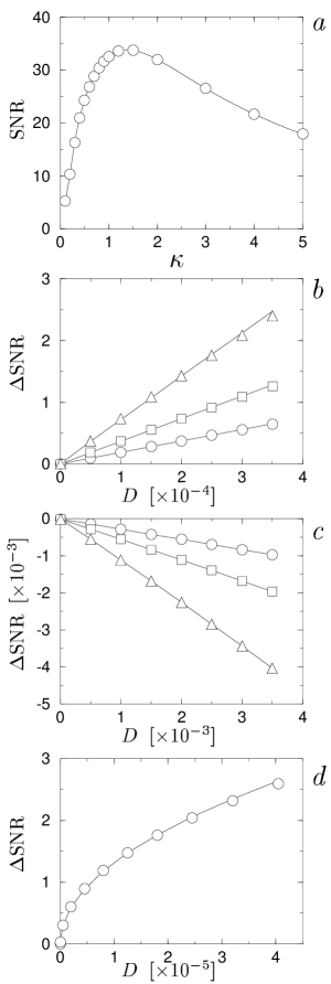
FIG. 1.: (a) SNR from the linearized SH equation as a function of $\kappa$ for $\alpha=1$, $q=1$, $\omega_{0}/2\pi=0.195$, and $g=1$. (b) $\Delta{\rm SNR}={\rm SNR}-{\rm SNR}(D=0)$ from Eq. (1) as a function of $D$ for $\kappa=0.3$, $q=1$, $\omega_{0}/2\pi=0.195$, and $g=0.5$ (circles), $g=1$ (squares) and $g=2$ (triangles). The points have been fitted by a power law, obtaining an exponent equal to $0.99$ for the three values of $g$. (c) $\Delta{\rm SNR}$ as in case b) but for $\kappa=3$. In this case the exponents of the power law are $0.99$, $1.00$, $1.02$. (d) $\Delta{\rm SNR}$ from Eq. (1) when replacing the nonlinear term by $g\psi|\psi|$, as a function of $D$ for $\kappa=0.3$, $q=1$, and $\omega_{0}/2\pi=0.195$, and $g=1$. In this case the scaling exponent is $0.50$. In all figures the size of the system is $32$.

FIG. 2.: (a) SNR and (b) $Q$ as functions of the noise level $D$ for $\alpha=1$, $\kappa=0.1$, $g=1$, $q=1$, and $\omega_{0}/2\pi=0.024$. The system size is $32$.

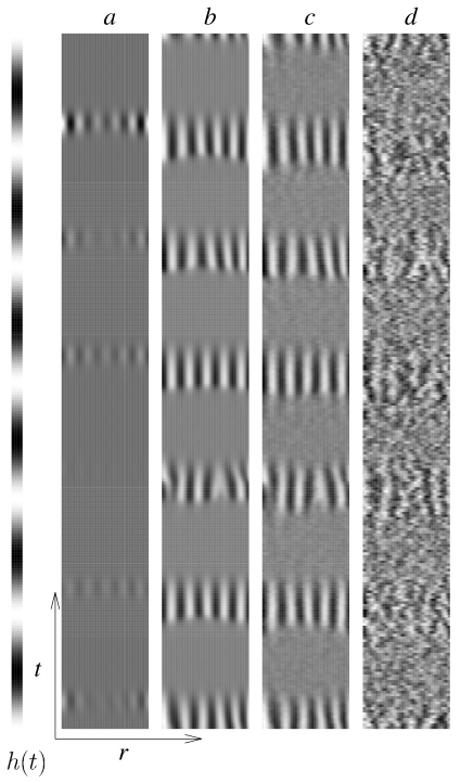
FIG. 3.: Spatiotemporal evolution of the one-dimensional SH equation with periodic boundary conditions for the noise levels (a) $D=0.5\times 10^{-15}$, (b) $D=0.5\times 10^{-4}$, (c) $D=0.5\times 10^{-2}$, and (d) $D=0.5$. The values of the remaining parameters are $\alpha=1$, $\kappa=0.1$, $g=1$, $q=1$, and $\omega_{0}/2\pi=0.024$. The system size is $32$. We have also indicated the time evolution of the control parameter $h(t)$. For each pattern, black and white colors stand for minimum and maximum values, respectively.

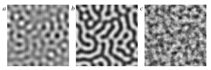
FIG. 4.: Representation of the field $\psi$ for the two-dimensional SH equation with periodic boundary conditions. The noise level is (a) $D=0.25\times 10^{-10}$, (b) $D=0.25\times 10^{-1}$, and (c) $D=2.5$. The remaining values of the parameters in all cases are $\alpha=1$, $\kappa=0.1$, $g=1$, $q=1$, and $\omega_{0}/2\pi=0.012$. The system size is $50\times 50$.

REFERENCES

- [1] R. Benzi, A. Sutera, and A. Vulpiani, J. Phys. A 14, L453 (1981).
- [2] B. McNamara, K. Wiesenfeld, and R. Roy, Phys. Rev. Lett. 60, 2626-2629 (1988);
- [3] B. McNamara and K. Wiesenfeld, Phys. Rev. A 39, 4854 (1989).
- [4] Proceedings of the NATO Advanced Research Workshop on Stochastic Resonance, San Diego, 1992 [J. Stat. Phys. 70, 1 (1993)].
- [5] F. Moss, in Some Problems in Statistical Physics, edited by G. H. Weiss (SIAM, Philadelphia,1994).
- [6] K. Wiesenfeld, D. Pierson, E. Pantazelou, C. Dames, and F. Moss, Phys. Rev. Lett. 72, 2125 (1994).
- [7] K. Wiesenfeld and F. Moss, Nature 373, 33 (1995).
- [8] Z. Gingl, L. B. Kiss, and F. Moss, Europhys. Lett. 29 191-196 (1995).
- [9] J. M. G. Vilar and J. M. Rubí, Phys. Rev. Lett. 77, 2863 (1996).
- [10] M. C. Cross and P. C. Hohemberg, Rev. Mod. Phys. 65, 851 (1993).
- [11] G. Ahlers in 25 Years of Non-Equilibrium Statistical Mechanics, J. J. Brey, J. Marro, J. M. Rubí and M. San Miguel (Eds) (Springer-Verlag, Lecture Notes in Physics, Berlin, 1995), p. 91.
- [12] P. Jung and G. Mayer-Kress, Phys. Rev. Lett. 74, 2130 (1995).
- [13] J. F. Lindner, B. K. Meadows, W. L. Ditto, M. E. Inchiosa, and A. R. Bulsara, Phys. Rev. Lett. 75, 3 (1995).
- [14] F. Marchesoni, L. Gammaitoni, and A. R. Bulsara, Phys. Rev. Lett. 76, 2609 (1996).
- [15] H. S. Wio, Phys. Rev. E 54, 3075R (1996).
- [16] J. B. Swift and P. C. Hohenberg, Phys. Rev. A 15, 319 (1977).
- [17] P. C. Hohenberg and J. B. Swift, Phys. Rev. A 46, 4773 (1992).
- [18] C. W. Meyer, G. Ahlers, and D. S. Cannell, Phys. Rev. A 44, 2514 (1991); 45, 8583 (1992).
- [19] W.H. Press, B. P. Flannery, S. A. Teukolsky, and W. T. Vetterling, Numerical Recipes (Cambridge University Press, New York, 1986).
- [20] P. E. Kloeden and E. Platen, Numerical Solution of Stochastic Differential Equations (Springer-Verlag, Berlin, 1995).
- [21] W. Van Saarloos and P. C. Hohenberg, Physica D 56, 303.