DIFFUSING RECONSTITUTING DIMERS: A SIMPLE MODEL OF BROKEN ERGODICITY AND AGEING

Abstract

We consider a model of assisted diffusion of hard-core particles on a line. In this model, a particle can jump left or right by two steps to an unoccupied site, but only if the the site in between is occupied. We show that this model is strongly non-ergodic, and the phase space breaks up into mutually disconnected sectors. The number of such sectors increases as the exponential of the size of the system. Within a sector, the model can be shown to be equivalent to the Heisenberg model, and is exactly soluble. We study how time-dependent autocorrelation functions in the model depend on the sector. We also show how this strong breaking of ergodicity ( which can be thought of as an infinity of conservation laws) affects the hydrodynamical description of the long wavelength density fluctuations in the system. Finally, we study the effect of allowing transitions between sectors at a very slow rate.

1 Slow and fast processes

If a system is weakly coupled to a heat bath at a given “temperature”, if the coupling is indefinite and not known precisely, if the coupling has been on for a long time, and if all the “fast” things have happened and all the “slow” things not, the system is said to be in thermal equilibrium. R. P. Feynman [1]

The Boltzmann-Gibbs method of calculating properties of a system of large number of interacting particles by defining a suitable ensemble of systems, and replacing the calculation of time-averages of obsevables by their phase space averages, is very powerful technique in statistical mechanics. To calculate the equilibrium properties of a system of a large number of degrees of freedom, all we have to do is to calculate the corresponding partition function, and thus the free energy. All quantities of interest can then be determined by taking derivatives of this free energy with respect to suitable conjugate fields. Of course, this calculation is quite nontrivial, involves evaluation of many-dimensional integrals, and can be exactly done only for a very small class of soluble models. However, standard approximation techniques, such as weak- or strong- coupling perturbation expansions, or variational schemes can be used to get answers which are as close to the correct answer as desired away from critical points, and near critical points other schemes such as renormalization group, $\epsilon-$ expansion etc. can be used to determine the behavior of different quantities. Thus, it is perhaps not an exaggeration to say that the general principles of determining equilibrium properties of systems are quite well understood by now.

However, many systems of interest, such as diamonds or ordinary glass, are not in thermal equilibrium, even though their properties do not seem to change significantly with time for the time-scale of experiments. These systems are said to be in metastable states. It is well realized that these states have much higher free energy than some other stable state of the system, and if the system could easily explore all parts of the phase space available to it, such states would occur with negligible probability. They owe their existence to the fact that the rate of transition to the stable phase can very low, and the system is not ergodic.

A precise microscopic specification of all positions and momenta of all the atoms, to describe the state of a small piece of glass is impossible. Clearly, we can, at best, hope to give a probabilistic description of the state. However, the ensemble of microscopic states having finite probability must to restricted to those which are ‘nearby’, and are accessible to the system within times comparable to the experimental time-scales. Such an ensemble in these systems is much smaller than the corresponding microcanonical ensemble. It is easy to see that phase space volume of accesible states of such a system occupies a negligible fraction of the full phase space, and this fraction decreases as $exp(-aV)$, as the volume of system $V$ increases. The coefficient $a$ seems to have only a very weak dependence on the time scale used to define the set of ’accessible’ states. Of course, $a$ must become zero as this time tends to the Poincare recurrence time of the system.

However, it has proved difficult to define this concept of restricted ensembles in a way which allows calculation of such partition functions, and thus determine the average properties of, even model systems. This is what we shall try to do here for a very simple toy model called the diffusing reconstituting dimers (DRD) model. The ideas developed in this paper have been discussed in a recent paper [2]. In this present paper, our aim is to argue that this is a very nice and tractable, hence useful model for glassy dynamics, while the earlier paper dealt more with its integrability, and connection to other soluble models. We shall not attempt to review here the very large body of work which already exists dealing with the phenomena of ageing and relaxation in spin glasses [3]. What is presented is a somewhat personal perspective.

The key observation here is note that the processes operating in a glass may be divided into two classes: fast and slow. Fast processes are those whose time scales are much shorter than that of observation, e.g. the vibratory motion of atoms about their mean positions. Slow processes are those involving rearrangement of atomic configurations, particle- or vacancy diffusion, creep etc. To define a quasi-equilibrium state of glassy systems, we have to imagine that “all the fast things have happened”, and the slow things have not even started. To be precise, we assume that the system dynamics is such that the slow processes do not occur at all. Then the dyanmics is nonergodic.

Figure 1: A schematic representation of the decomposition of phase space into disconnected sectors. The points denote different configurations. Full lines show allowed fast transitions between sectors. Different sectors are enclosed in rectangular boxes. Dotted lines show slow transitions between different sectors.

The phase space breaks up into a large number of disconnected pieces, called sectors. The number of such sectors increases exponentially with the size of the system. We shall call such system many-sector decomposable (MSD), and the ensembles which sum over only one of these sectors as pico-canonical ensembles.

For the toy model we consider, partition functions corresponding to such pico-canonical ensembles can be explicitly computed. These differ from sector to sector. As the number of sectors is of the order of $exp(V)$, a precise specification of the sector is too microscopic a detail, and not relevant. In an experiment, one can, at best, hope to give some general probabilistic characterization of the sector. This presumably would depend on the history, and preparation of the system, e.g. cooling schedules etc.. In a theoretical calculation, this implies that once the free energy in the pico-canonical ensemble is determined, it must then be further averaged over sectors with a suitable weight for each sector.

Finally, we shall show how we can describe the phenomena such as ageing in glasses by taking into account the slow processes, as providing a stochastic dynamics in which the system jumps from one sector to another in time, and thus brings back ergodicity ( or tries to ) at very large times.

2 The Model

The model we shall choose to address these issues is a very simple one. We consider $N$ hard-core point particles on a linear chain of $L$ sites. There are no interactions amongst the particles except the hard-core interaction. We assume that the system evolves in continuous time time by a local Markovian dynamics. We shall choose the transition rates to satisfy the detailed balance condition, so that the rate from a transition, say from configuration $C$ to $C^{\prime}$, is the same as the rate of the reverse transition $C^{\prime}$ to $C$. Then, in the steady state all accessible configurations occur with equal probability.

Now for a more detailed specification of the allowed transitions. We assume that the particles can diffuse to nearby sites, but only if there is another particle nearby: a case of assisted diffusion. More precisely, a particle at site i can jump left or right by two steps to the sites $i{\pm}2$, if that site is unoccupied, and the in-between site $i{\pm}1$ is occupied. If allowed, this transition occurs at rate 1. We represent the configuration of the system by a binary string $01100100$…. of length $L$, where the $i^{th}$ bit gives the occupation number $n_{i}$ of the site $i$. Then this process can be represented by a ‘chemical’ equation

$$110{\leftarrow\rightarrow}011$$

An alternate way of viewing the system is to say that isolated particles cannot diffuse. But two particles at adjacent sites can diffuse together one step to the left or right with rate $1$. These pairs of particles will be called dimers. However, these pairings are not for ever, and the dimers can ‘reconstitute’. Thus, for example, in the sequence of transitions

$$..11010..{\rightarrow}..01110..{\rightarrow}..01011..$$

the middle particle is first paired with particle on the left, and then in the second transition with the particle on the right. We are thus considering a system of Diffusing Reconstituting Dimers (DRD).

A third possible way of looking at the model is to think of the diffusion as that of 0’s by two steps left or right if the intervening site is not a zero. This is then not assisted diffusion, but too many zeroes will ‘hinder’ each other’s diffusion.

The assumption in the model monomers have a much lower diffusivity than dimers is not easily realized in real physical systems. However, instances where this happens are not unknown: for example, platinum dimers on some surfaces have higher mobility than monomers.

3 Many Sector Decomposition and Conservation Law of the Irreducible String

For of linear chain of L sites, the phase space consists of $2^{L}$ distinct configurations. It is however clear that the dynamical rules are such that the system is not ergodic. For example, the as the diffusion process conserves the number of particles, a system starting with N particles at some time will never be found in a configuration with a different number of particles. The phase space thus breaks up into mutually disconnected subsets, called sectors. The stochastic evolution of the system takes it from one configuration to another, within the same sector, but no transitions are allowed between different sectors.

The conservation of particle number implies that the total phase space can be broken into $(L+1)$ disconnected subsets, each subset specified by a different value of the total particle number. Such conservation laws are well known in equilibrium statistical mechanics, and there effect is easily taken into account by defining suitably restricted ensemble : say the canonical ensemble in which the number of particles is fixed. In addition, usually, one can prove that there is an equivalence of different ensembles ( except at special points like when the system is at a phase transition point). So one can even work with ensemble having a variable number of particles, so long as the chemical potential is chosen so that the average density comes out right.

But this is not all. It is easy to see that if we break the linear chain into two sublattices (even and odd), then number of particles on each sublattice is separately conserved. Thus the phase space has to be broken up further. Most of the $(L+1)$ subspaces have to further subdivided into roughly L parts, so that the total number of disconnected regions of phase space is now of order $L^{2}$. This would imply that to describe the long-time steady state of the system correctly, one would need not one, but two chemical potentials, one for each sublattice, and adjust them so that the initial state density on each sublattice is correctly reproduced.

So long as the number of conserved quantities is finite, one can continue this process, and eventually end up with a system described by conventional Gibbs measure on a suitably defined ‘microcanonical’ ensemble in the phase-space, or equivalently a ‘canonical’ ensemble where the conservation laws are ignored, but their effects taken into account by including a finite number of thermodynamic potentials [4]. If there are m conserved quantities, and each takes order $L$ distinct values, the phase space has order $L^{m}$ distinct sectors.

However, it is easy to see that in the DRD model, the breaking of ergodicity is much more severe. In fact the number of disconnected sectors increases as exponential of L. This is easy to see. Consider a configuration in which there are no adjacent sites both occupied such as

$$...0010100010010000101.....$$

From the rules of the DRD dynamics, such a configuration cannot evolve at all, and remains the same at all times. The number of such configurations is easily shown to grow exponentially with $L$. [It is easy to show that this grows as ${\mu}^{L}$, where $\mu$ is the golden mean =1.618…]

Figure 2: A non-trivial sector with L=9, and five states within the sector. The arrows indicate allowed transitions between these. For this sector the irreducible string is $1010010$.

Consider now a less trivial case of single diffusing dimer in a frozen background. This is shown in fig. 2. We see that while the movable $1$’s change in time, as the dimer reconstitutes as it moves, there is exactly one movable dimer in each such configuration if you want to move to the right, and exactly one (possibly different) if you want a leftward move. After an order L moves in one direction, one reaches the end, and no further moves are possible. So there are about L configurations in each such sector. The number of sectors again grows as ${\mu}^{L}$.

It is possible to continue this process, and construct sectors in which $2,3,..$ movable dimers are present. To get a full description of the phase-space decomposition, we need to develop a systematic method for doing this. This is most conveniently done in terms of a construction called the irreducible string (IS), which we describe next.

With each of the $2^{L}$ possible configurations of the DRD model, we attach a binary string, called the IS corresponding to that configuration, constructed as follows: We take the $L$-bit binary string of ${n_{i}}$ specifying the configuration. We read this string from left to right until the first pair of adjacent $1$’s is encountered. This pair is deleted, reducing the length of the string by $2$. We repeat this process until no further deletions are possible. The resulting string is the IS for the configuration. For example, for the binary string $01001110110$, the irreducible string is $0100100$.

By construction, for each configuration, there is a unique IS. However, many different configurations may yield the same IS. The usefulness of this construction stems from the following observation: Two different configurations belong to the same sector, if and only if they both have the same IS. This is easy to see.

Firstly, we note that we need not assume that the pair of $1$’s to be deleted has to be the first occurrence of consecutive $1$’s when read from left to right. We get the same IS, whatever the choice and order of pairs $11$ deleted, so long as the final string has no pairs of $1$’s in it. [For example, from the configuration $101110$, we get the same IS $1010$, whether the second and third $1$’s, or the third and fourth $1$’s are deleted.] Then, if we get configuration $C^{\prime}$ from $C$ in one elementary step, deleting the diffusing dimer first, we see that both $C$ and $C^{\prime}$ have the same IS. Thus, the IS is a constant of motion.

Secondly, if two configurations $C$ and $C^{\prime}$ have the same IS, then there exists a sequence of allowed transitions of the DRD model, which takes $C$ to $C^{\prime}$.To prove this, notice that we can push any diffusing dimer in $C$ as far right as possible, and get a standard configuration in the sector, in which the configuration is the IS followed by all the dimers. Thus, for example, the standard configuration corresponding to the configuration $101110$ is $101011$. Corresponding to the configuration $01001110110$, it is $01001001111$. If $C$ and $C^{\prime}$ have the same IS, they can both be transformed into the same standard configuration, and as the DRD rules are reversible, into each other. So they belong to the same sector.

The conservation of the IS thus gives us a convenient way to label the different sectors of the DRD model. To each allowed IS corresponds a unique sector. In addition, this decomposition of phase space into disjoint sectors using the IS as a constant of motion is maximal in the sense that there are no other independent constants of motion.

As a side remark, let us note that the number of independent constants of motion is not a well-defined concept for a discrete system. For a classical mechanical system with n-dimensional phase space, we say that there are r independent constants of motion if the trajectories are confined to (n-r) dimensional manifolds. But for systems with discrete phase space, the trajectory consists of a finite number of discrete points, and its dimension is undefined.

In fact, for such a system, given two independent constants of motion $I_{1}$ and $I_{2}$, one can always construct a third single constant of motion $I_{3}$, such that both $I_{1}$, and $I_{2}$ are known functions of $I_{3}$. This result was proved in the context of quantum mechanics, by von Neumann [5] (for a recent discussion see Wiegert [6]). His argument is quite simple, but does not seem to be as well known as it should be. Consider $I_{1}$, $I_{2}$ as two given commuting quantum mechanical observables over a finite dimensional Hilbert space. Since $I_{1}$ and $I_{2}$ are mutually commuting, they can be simultaneously diagonalized. Then the quantum-mechanical Hilbert space of all possible states of the system can be represented as a direct sum of subspaces, each of which corresponds to a pair $(\lambda_{1},\lambda_{2})$, where $\lambda_{1}$ and $\lambda_{2}$ are eigenvalues of the operators $I_{1}$ and $I_{2}$. We order these subspaces in an arbitrary order, and define the operator $I_{3}$ to be block diagonal in this basis, with eigenvalue $r$ for all eigenvectors in the $r^{th}$ subspace. Then, by construction, This operator commutes with both $I_{1}$ and $I_{2}$, and its eigenvlaue $r$ tells us the sector, and hence both $\lambda_{1}$ and $\lambda_{2}$. Thus, the operators $I_{1}$ and $I_{2}$ are functions of $I_{3}$.

Using the von Neumann construction, we can take any set of commuting constants of motion $I_{1},I_{2},I_{3},...$, and collapse them into a single constant. In general, if one can construct an observable which takes the same value for all configurations within a sector, but distict values in distinct sectors, then such an observable is a constant of motion and there can not exist any other constants of motion independent of it. Conversely, a single constant of motion having $2^{n}$ distinct eigenvalues can be thought of as n independent constants of motion, each having only two distinct eigenvalues.

For the DRD model, this implies that the IS can be thought of as a single constant of motion, equivalent to a large number of independent constants of motion: If we count the number of 1’s between the $i^{th}$ and $(i+1)^{th}$ zero in the binary string corresponding to the configuration, with time this number can only change in multiples of 2, hence its parity is conserved. If one is uncomfortable with constants of motion whose values are character-strings, the IS can be thought of as a binary integer.

There is another way to represent the IS as a constant of motion, which makes contact with the theory of integrable models. We consider two noncommuting matrices $A(0)$ and $A(1)$ ( these can in general be complex $n\times n$ martices, but may be taken to be $2\times 2$ real matrices for our purpose here) which satisfy the relation

$$A(1)A(1)A(0)=A(0)A(1)A(1)$$ (1)

For any configuration $C$ of the DRD model with occupation numbers ${{n_{i}}}$, we define a matrix $I_{L}(C)$ by

$$I_{L}(C)=\prod_{j=1}^{L}A(n_{j})$$ (2)

where the matrix product is ordered so that larger $j$ values are more to the right. Then, from the eq(1) it follows that this matrix product does not change by an elementary evolution step of the DRD model. This implies that $I_{L}$ will not change in time even as $C$ changes, and thus is a contant of motion. Eq(1) does not completely determine $A(0)$ and $A(1)$, as these forms only $4$ equations for $8$ real parameters making the marices $A(0)$ and $A(1)$. Thus we can choose a one parameter family of matrices $A(0,\lambda)$ and $A(1,\lambda)$ depending on a real parameter $\lambda$. A simple specific choice is

$$A(0,\lambda)=\left[\begin{array}[]{clcr}1-\lambda&\lambda\\ 1&-1\end{array}\right]$$ (3)

and

$$A(1,\lambda)=\left[\begin{array}[]{clcr}1&0\\ 0&-1\end{array}\right]$$ (4)

Now $I_{L}$ becomes a 2X2 matrix of the form

$$I_{L}(C,\lambda)=\left[\begin{array}[]{clcr}I_{11}(\lambda)&I_{12}(\lambda)\\ I_{21}(\lambda)&I_{22}(\lambda)\end{array}\right]$$ (5)

whose elements $I_{11},I_{12},I_{21}$ and $I_{22}$ are polynomials in $\lambda$ of degree at most $L$. Since this matrix is conserved for all values of $\lambda$, it follows that all the coefficients of these polynomials are constants of motion. These coefficients in terms can be written out explicitly as functions of ${n_{i}}$.

4 Equivalence to a Multi-Species Exclusion Process

The algorithm to determine the IS also specifies the positions of the characters in the L-bit binary string that remain undeleted. As the configuration evolves, these positions will change, but the relative order of the characters remains unchanged. The DRD model can thus be viewed as a process of diffusion of hard-core particles on a line. Let the IS be of length $\ell$. Then the number of particles is $\ell$. Let $X_{i}(t)$ be the position of the $i^{th}$ character of the IS (counting from left). Each particle carries with it a ‘spin label’ which is 0 or 1, and is unaffected by the dynamics. Thus, our model is a special case of the Hard-Core Random Walkers with Conserved Spin (HCRWCS) models which may be defined for all 1-d models where a conserved IS can be defined [7, 8, 9, 10].

If the $i^{th}$ character of the IS is a 1, it must be followed by a 0 in the IS, and also on the chain, this character must be immediately after it. so that we have

$$X_{i+1}(t)=X_{i}(t)+1$$

for all times t, and the $i^{th}$ and $(i+1)^{th}$ walkers always move together. In this case it is better to think of these as a single walker, which occupies two consecutive sites on the chain. Then there are two kinds of walkers: walkers with spin label 0 occupying a single site, and walkers with label 10 which occupy two sites. In addition there are the sites not occupied by the random walkers, which are occupied by dimers 11, which again occupy two sites. Let us call these particles of type $B$,$C$ and $A$ respectively. We now show that the DRD dynamics can be viewed as a stochastic dynamics of a system of 3 species $A$, $B$ and $C$ of particles on a line. In the latter process ( to be called the Exclusion process (ExP)), each site of linear chain is occupied by a single particle, which may be of type $A$, $B$, or $C$. We set up a one-to-one correspondence between the configurations of the DRD model, and of the ExP as follows: Read the binary string of the DRD from left to right. If the next character of the DRD model is 0, another character in the DRD string is read.We write a single character $A$ or $B$ for the ExP string, depending on if the last chacter read was $1$ or $0$. Conversely, the binary string corresponding to a configuration $ABBCAABCB$… of the ExP is obtained by a simple substitution $A\rightarrow 11$, $B\rightarrow 10$, $C\rightarrow 0$.

We can now write the stochastic evolution rule in terms of the ExP configurations. These are quite simple: A particle of type $A$ can exchange position with a particle of type $B$ or $C$ at an adjacent site with rate 1. Type $B$ and $C$ cannot exchange positions with each other. This model thus is a special case of the k-species exclusion process defined by Boldrighini et al [11]. In the latter, there are k distinct species of particles (k=2,3,4..). and particles can exchange places with adjacent particles with a rate which depends on both the species of the particles beinf interchanged. In our case k=3. The k-species model has been studied recently Derrida et al [12], and by Ferrari et al [13].

The conservation of IS in this language corresponds to the simple statement that as $B$ and $C$ type particles cannot exchange places, their relative order is unchanged in time. Consider a string composed of three characters $A$, $B$ and $C$ which specifies a configuration of the ExP process. Then deleting all the occurrences of $A$’s in the string, we are left only with a string composed of $B$’s and $C$’s which is conserved by the dynamics.

5 Calculation of the Number and Sizes of Sectors

In terms of the ExP model, it is quite straightforward to write down the formulas for the number of distinct sectors for the DRD model, and also the number of configurations in each sector. Consider free boundary conditions for convenience. In a sector having $N_{A}$ particles of type $A$, $N_{B}$ particles of type B, and $N_{C}$ particles of type $C$, the total number of sites is $L=2N_{A}+2N_{B}+N_{C}$. The number of 1’s in this case is $2N_{A}+N_{B}$, and the number of 0’s is $N_{B}+N_{C}$. The length of the IS is $2N_{B}+N_{C}$.

The number of distinct sectors is the number of distinct ways of writng the IS consisting of $N_{B}$ $B$’s and $N_{C}$ $C$’s. Since all choices are allowed, this is $(N_{B}+N_{C})!/(N_{B}!N_{C}!)$. The number of configuration within a sector with a specified IS, say $BCCCBBCBC$…., is the number of ways we can place $N_{A}$ $A$’s between $(N_{B}+N_{C})$ $B$’s and $C$’s. So this number is

$$\Omega(N_{A},N_{B},N_{C})=(N_{A}+N_{B}+N_{C})/[N_{A}!(N_{B}+N_{C})!]$$ (6)

This determines the picocanonical entropy in each sector. To calculate the total number of sectors, we have to sum the number of sectors over all allowed values of $N_{B}$ and $N_{C}$.

Multiplying $\Omega(N_{A},N_{B},N_{C})$ by the number of sectors with $N_{B}$ B-type and $N_{C}$ C-type particles, we get the the total number of configurations having $N_{A},N_{B}$ and $N_{C}$ particles of type A,B,C respectively. Denote this by $\Xi(N_{A},N_{B},N_{C})$. Then we get

$$\Xi(N_{A},N_{B},N_{C})=(N_{A}+N_{B}+N_{C})!/[N_{A}!N_{B}!N_{C}!]$$ (7)

Extremizing this with respect to $N_{A},N_{B}$ and $N_{C}$, subject to the constraint that $2N_{A}+2N_{B}+N_{C}=L$, we see that the this is extremized for $N_{A}=N_{B}=N_{C}/2=L/6$. Hence if we pick a configuration at random, its length is most likely to be approximately $2L/3$, and it will have approximately $L/6$ diffusing dimers. The typical number of configurations in this sector is ${\kappa}^{L}$ where ${\kappa}=2^{4/3}.3^{-1/2}$. The number such sectors is approximately ${\kappa}^{\prime L}$, where ${\kappa}^{\prime}=3^{1/2}.2^{-1/3}$. [ We check that ${\kappa\kappa}^{\prime}=2$, so that the total number of configurations increases as $2^{L}$, as it must.]

Alternatively, we can proceed directly as follows: Let $F_{\ell}(0)$ and $F_{\ell}(1)$ be the number of distinct strings of length $\ell$ which end in a $0$ and a $1$ respectively. Since in the IS, a $1$ must be followed by $0$, by a $0$ may be followed by either $0$ or $1$, these F’s satisfy the recursion relations

$$F_{\ell+1}(0)=F_{\ell}(0)+F_{\ell}(1)$$ (8)

$$F_{\ell+1}(1)=F_{\ell}(0).$$ (9)

Given the starting values $F_{1}(0)=F_{1}(1)=1$ these recursions are easily solved, and we see the $F_{\ell}(1)$ is the ${\ell}^{th}$ Fibonacci number which grows as ${\mu}^{\ell}$, where $\mu=(\sqrt{5}+1)/2$. For a line of length L, the largest possible value of $\ell$ is L. A sector with $r$ diffusing dimers corresponds to $\ell=L-2r$. Hence the total number of sectors is

$$N_{L}=\sum_{r=0}^{[L/2]}[F_{L-2r}(0)+F_{L-2r}(1)]$$ (10)

where $[L/2]$ is the largest integer not greater than $L/2$. This shows that the total number of sectors also increase as ${\mu}^{L}$ for large $L$.

For the DRD model, the probability weights in the steady state correspond to the rather trivial Hamiltonian H=0, and so the calculation above does not seem to have much interesting structure, or variation from sector to sector. But it does provide us with a simple system where one can completely characterize different sectors, and calculate phase-space averages within a specified sector.

6 The Rate matrix as a Quantum Spin Hamiltonian

The technique of writing down a quantum-spin hamiltonian corresponding to a Markov process for a discrete system is by now quite well-known [14]. For completeness, we recapitulate it here briefly. Let $P({\cal C},t)$ be the probability that a classical system undergoing Markovian evolution is in the configuration ${\cal C}$ at time $t$. These probabilities evolve in time according to the master equation

$${\partial P({\cal C},t)\over\partial t}=\sum_{{\cal C}^{\prime}}\left[-W({\cal C}\rightarrow{\cal C}^{\prime})\,P({\cal C},t)+W({\cal C}^{\prime}\rightarrow{\cal C})\,P({\cal C}^{\prime},t)\right]$$ (11)

where the summation over ${\cal C}^{\prime}$ is over all possible configurations of the system and $W({\cal C}\rightarrow{\cal C}^{\prime})$ is the transition rate from configuration ${\cal C}$ to configuration ${\cal C}^{\prime}$.

We define a Hilbert space, spanned by basis vectors $|{\cal C}\rangle$, which are in $1$ to $1$ correspondence with the configurations ${\cal C}$ of the system. A configuration with probability weight $P({\cal C},t)$ is represented in this space by a vector

$$|P(t)\rangle=\sum_{{\cal C}}P({\cal C},t)|{\cal C}\rangle$$ (12)

The master equation can then be written as

$${\partial|P(t)\rangle\over\partial t}=-{\hat{H}}|P(t)\rangle$$ (13)

This equation can be viewed as an imaginary-time Schodinger equation for the evolution of the state vector $|P(t)\rangle$ under the action of the quantum Hamiltonian ${\hat{H}}$.

The $2^{L}$ configurations of the DRD model on a line of length $L$ can be put in one-to-one correspondence with the configurations of a spin-$1/2$ chain of $L$ sites. At the site $i$, the spin variable is $\sigma_{i}^{z}=2n_{i}-1$, and takes values $+1$ and $-1$ if $n_{i}$ is $1$ or $0$ respectively. It is then straightforward to write ${\hat{H}}$ as the Hamiltonian of the spin chain in terms of the Pauli spin matrices $\sigma_{i}$. We find that ${\hat{H}}$ has local 2-spin and 3-spin couplings, and is given by

$${\hat{H}}=-\frac{1}{4}\sum_{i}\left[\vec{\sigma}_{i-1}\cdot\vec{\sigma}_{i+1}-1\right]\,(1+\sigma^{z}_{i})$$ (14)

This Hamiltonian is quite similar in structure to an integrable spin model with three-spin couplings proposed and solved by Bariev[15]. The Bariev model has the Hamiltonian given by

$$\hat{H}_{B}=-{1\over 4}\sum_{i}(\sigma^{x}_{i-1}\sigma^{x}_{i+1}+\sigma^{y}_{i-1}\sigma^{y}_{i+1})(1-U\sigma^{z}_{i})$$ (15)

The sign of $U$ can be changed by the transformation $\sigma^{x}_{i}\rightarrow\sigma^{y}_{i}$, $\sigma^{y}_{i}\rightarrow\sigma^{x}_{i},$ and $\sigma^{z}_{i}\rightarrow-\sigma^{z}_{i}$. We set $|U|=1$. Then the Bariev model differs from our model through the term

$$\hat{H}-\hat{H}_{B}=H^{\prime}=-{1\over 4}\sum_{i}\left(\sigma^{z}_{i-1}\sigma^{z}_{i+1}-1\right)\left(1+\sigma^{z}_{i}\right)$$ (16)

It is easy to see that these terms commute with the IS operator $\hat{I}_{L}(\lambda)$. Thus $\hat{I}_{L}(\lambda)$ also commutes with $\hat{H}_{B}$, and provides an infinity of constants of motion of the Bariev model (in the special case $|U|=1$).

It is useful to write this Hamiltonian in terms of fermion operators $c^{+}_{i}$ and $c_{i}$ defined by the Jordan-Wigner transformation

$$c^{+}_{i} = \exp\left[-i\pi\sum^{i-1}_{j=1}\sigma^{+}_{j}\sigma^{-}_{j}\right]\,\sigma^{+}_{i}$$

$$c_{i} = \exp\left[i\pi\sum^{i-1}_{j=1}\sigma^{+}_{j}\sigma^{-}_{j}\right]\,\sigma^{-}_{i}$$ (17)

In terms of these fermion operators, ${\hat{H}}$ can be written as

$${\hat{H}}=\sum_{i}\left[c^{+}_{i-1}n_{i}c_{i+1}+c^{+}_{i+1}n_{i}c_{i-1}+n_{i}(n_{i-1}-n_{i+1})^{2}\right]$$ (18)

where $n_{i}=c^{+}_{i}c_{i}$ is the number operator at site $i$. The first two terms of this Hamiltonian represent assisted hopping over an occupied site, and the last term describes two- and three- body potential interaction between nearby sites. Similar hopping terms are encountered in a model studied by Hirsch in the context of hole superconductivity[16].

7 Conservation laws of the Quantum Hamiltonian

While the evolution of probabilities in a classical Markov process could be cast as the evolution of the wavefunction of a suitably defined quantum mechanical problem, the concept of constants of motion is quite different in these two cases, as I explain below.

A classical observable ${\cal O}$ is a function which assigns a value, say in terms of a real number ${\cal O}({\cal C})$ to each possible configuration ${\cal C}$ of the system. We say that ${\cal O}$ is a constant of motion when the value of the observable ${\cal O}({\cal C}_{t})$, associated with the configuration of the system ${\cal C}_{t}$ at any arbitrary time $t$, is independent of $t$. In a quantum mechanical formulation, observables are represented by matrices $\hat{\cal O}$, and the quantity of interest is the expectation value of the observable ${\cal O}$ at time $t$, given by the formula

$$\langle\hat{\cal O}\rangle_{t}=\langle 1|\hat{\cal O}|P(t)\rangle,$$ (19)

where $\langle 1|$ is the row vector with all entries 1. Clearly, in this language, a classical observable ${\cal O}$ corresponds to a quantum mechanical operator $\hat{\cal O}$, which is diagonal in the natural basis of the system, i.e. when the basis vectors are $|{\cal C}\rangle$.

We shall call a quantum mechanical observable $\hat{\cal O}$ a constant of motion, if the matrix $\hat{\cal O}$ commutes with the Hamiltonian ${\hat{H}}$. In this case it is easy to verify that its expectation value evaluated with respect to the probability vector $|P(t)\rangle$ does not change in time. (Note that we are using a different prescription for evaluating expectation values than in standard quantum mechanics.) Clearly the class of all possible quantum mechanical constants of motion (all matrices $\hat{\cal O}$) is much larger than that of the classical constants of motion (diagonal in the configuration basis).

We have already seen that the IS is a classical constant of motion. Using its definition, (Eq. 4.5), we define the diagonal matrix $\hat{I}_{L}(\lambda)$ by

$${\hat{I}}_{L}(\lambda)=\prod^{L}_{j=1}A({\hat{n}}_{i},\lambda),$$ (20)

where ${\hat{n}}_{j}=\sigma^{+}_{j}\sigma^{-}_{j}$ is now an operator, and not a c-number. It is easy to verify that ${\hat{H}}$ commutes with ${\hat{I}}_{L}(\lambda)$ , for all values of $\lambda$. Thus ${\hat{I}}_{L}(\lambda)$ provides us with a one parameter family of constants of motion. In fact, as discussed earlier, there are no additional independent classical constants of motion in our model.

As ${\hat{H}}$ commutes with ${\hat{I}}_{L}(\lambda)$, it has a block-diagonal structure, with each block corresponding to a sector of the phase space, and to a particular IS. The task of diagonalizing ${\hat{H}}$ then reduces to that of diagonalizing it in each of the sectors separately.

Consider any one of these sectors. Let the IS ${\cal I}$ for this sector, in the 3-species exclusion process notation, be a string of $N_{B}\,B$’s and $N_{C}\,C$’s in some order, say ${\cal I}=BCBBCBCC\ldots$ The number of diffusing dimers in this sector then is $N_{A}=(L-2N_{B}-N_{C})/2$. A typical configuration in this sector is specified by a string of length $(N_{A}+N_{B}+N_{C})$ with $N_{A}\,A$’s interspersed between the characters of the IS, e.g. BCABAABCBCAC $\ldots$.

We define a chain of spin-1/2 quantum spins ${\tau_{i}}$, with $i$ ranging from $1\/$ to $L_{\tau}=(N_{A}+N_{B}+N_{C})$. For each configuration in the sector ${\cal I}$, we define a corresponding configuration of the $\tau$-spin chain by the rule that $\tau_{j}^{z}=+1$ if the $j^{\rm th}$ character in the string specifying the configuration is $A$. For $\tau^{z}_{j}=-1$, the corresponding character can be either $B$ or $C$. But this degeneracy is completely removed by using the known order of these elements in the irreducible string ${\cal I}$. Thus there is a one-to-one correspondence between the configurations of the DRD model in the sector ${\cal I}$, and the configurations of the $\tau$-chain with exactly $N_{A}$ spins up.

The action of the Hamiltonian $\hat{H}$ on the subspace of configurations in the sector ${\cal I}$ looks much simpler in terms of the $\tau$-spin variables. It is easily checked that the evolution in terms of the $\tau$-variables is that of a simple exclusion process. The quantum Hamiltonian for this process is the well known Heisenberg Hamiltonian

$${\hat{H}}_{Heis}=-\sum^{L_{\tau}-1}_{i=1}\left(\vec{\tau}_{i}\cdot\vec{\tau}_{i+1}-1\right).$$ (21)

Note that ${\hat{H}}_{Heis}\/$ looks different for sectors with differing $\L_{\tau}$’s. We have defined the transformation between the $\sigma-$ and $\tau-$ spin variables by an algorithmic prescription. It seems very difficult to do so by an explicit formula. The transformation is very complicated, and non-local.

We would now like to construct a one-parameter family of operators that commute with ${\hat{H}}_{Heis}$. This is a well-known construction for the Heisenberg model [17]. We use periodic boundary conditions for convenience. Define $2\times 2$ matrices $L_{j}(\mu)$ whose elements are operators acting on the spin $\tau_{j}$, and $\mu$ is a parameter

$$L_{j}(\mu)=\Biggl{(}\matrix{1+i\tau_{j}^{z}\mu&i\mu\tau^{-}_{j}\cr i\mu\tau_{j}^{+}&1-i\tau^{z}_{j}\mu}\Biggr{)},$$ (22)

and define

$$\hat{\cal T}(\mu)=Tr\prod^{L_{\tau}}_{j=1}L_{j}(\mu).$$ (23)

Then it can be shown that [17] for all $\mu,\mu^{\prime}$

$$\left[\hat{\cal T}(\mu),\hat{\cal T}(\mu^{\prime})\right]=0.$$ (24)

Writing $\ln\hat{\cal T}(\mu)=\sum^{\infty}_{r=1}\mu^{r}\hat{J}_{\mu}$ we get $\left[\hat{J}_{r},\hat{J}_{s}\right]=0$, for all $r,s$ and $\hat{J}_{2}={\hat{H}_{Heis}}$. Thus the set of operators $\{\hat{J}\}$ constitute a set of quantum mechanical constants of motion for the Hamiltonian ${\hat{H}}_{Heis}\/$ in each sector separately, and hence for ${\hat{H}}\/$.

The Hamiltonian ${\hat{H}}$ has still another additional infinite set of constants of motion. These are related to the existence of an additional symmetry in the model. Clearly, replacing a $B$-type particle by a $C$-type particle does not affect the dynamics of the exclusion process. Thus, the full spectrum of eigenvalues of ${\hat{H}}$ in any two sectors of the DRD model with different irreducible strings, but having the same values of $N_{A}$ and $N_{B}+N_{C}$, is exactly the same. Such a symmetry may be viewed as a local gauge symmetry between the $B$ and $C$ ‘colors’. Changing the character in the IS from $B$ to $C$ (or vice versa) changes the length of $L$ by 1. This symmetry therefore relates two sectors of the DRD model with different sizes of the system.

The simplest inter-sector operators which preserve the total length of the chain $L$ are operators which interchange two characters of the IS. Let ${\hat{K}}_{j}$ be the operator which interchanges the $j^{\rm th}$ and $(j+1)^{\rm th}$ characters of the IS. Then clearly, we have

$$\left[{\hat{H}},{\hat{K}}_{j}\right]=0\,\,{\rm for}\,\,j=1\,\,{\rm to}\,\,L_{\tau}-1.$$ (25)

This ‘color’ symmetry implies that the spectrum of ${\hat{H}}$ is the same in all the sectors with the same value of $L$ and $N_{A}$.

We have thus shown that the DRD hamiltonian shows the existence of three different classes of infinity of constants of motion: the classical-mechanical constants of motion which may be encoded in the conservation of IS, the off-diagonal constants of motion of the Heisenberg model which can be used to diagonalize the martix ${\hat{H}}$ within a sector, and the constants of motion ${\hat{K}}$ which are also off-diagonal, but relate eigenvalues and eigenvectors in different sectors.

8 Time-dependent Correlation Functions

The static correlation functions in the DRD model are quite trivial because of the simple form of the hamiltonian chosen. The effect of ergodicity- breaking and constrained evolution is best seen in the time- dependent density autocorrrelation functions. These show interesting variations from one sector to another. Such variations occur despite the fact that, in each sector, there is a mapping between the DRD model and the simple exclusion process whose dynamics is known to be governed by diffusion. As we will see below, this mapping leads to a correspondence between tagged hole correlation functions in the two problems, but the form of autocorrelation function decays depends on the IS, and can be quite different.

Consider a particular sector with IS ${\cal I}$. Let the number of diffusing A, B and C particles in the equivalent 3-species exclusion process be $N_{A},N_{B}$ and $N_{C}\/$ respectively. In the IS, let $b(k)$ be the number of B’s to the left of the k-th hole.( A hole is a particle of type $B$ or $C$.) Evidently, the function $b(k)$ specifies the IS completely.

Different configurations in the sector are obtained from different distributions of A’s in the background of B’s and C’s. If there are $a_{k}$ A’s to the left of the k’th hole, the location of this hole in the ExP and DRD problems is

$$y_{ExP}(k,t) = k+a_{k}(t),$$ (26)

$$y_{DRD}(k,t) = k+b(k)+2a_{k}(t).$$ (27)

Notice that $b(k)$ (unlike $a_{k}$) is time-independent. Defining a tagged-hole correlation function for the ExP and DRD problems in analogy with the conventional tagged-particle correlation function[18] through

$$\sigma^{2}(t)=<[y(k,t)-y(k,0)]^{2}>,$$ (28)

we see that the simple relationship

$$\sigma_{DRD}(t)=2\sigma_{ExP}(t)$$ (29)

holds. However, no simple, exact equivalence between the two problems can be established for tagged-particle correlations or single-site autocorrelation functions. This is because the transformation between spatial coordinates in the DRD and related ExP problems is nonlinear; a fixed site in the former problem corresponds to a site whose position changes with time in the latter.

Let $x\/$ and $\xi\/$ denote spatial locations in the DRD and ExP problems respectively and let $a_{\xi}$ be the number of A’s to the left of $\xi$. Evidently, the number of holes (B’s and C’s) to the left of this site is $(\xi-a_{\xi})\/$. In the equivalent configuration in the DRD problem, each A corresponds to two particles, while the $(\xi-a_{\xi})\/$ B’s and C’s occupy a length $b(\xi-a_{\xi})+\xi-a_{\xi}\/$ which depends on the IS in question. Thus

$$x=a_{\xi}+b(\xi-a_{\xi})+\xi,$$ (30)

while the number of particles $a_{x}$ to the left of $x$ is given by

$$a_{x}=2a_{\xi}+b(\xi-a_{\xi}).$$ (31)

The transformation between the integrated particle densities $a_{x}$ and $a_{\xi}$ is therefore quite complicated. It depends on the IS through the function $b\/$ and is highly non-linear.

The correlation functions involving $a_{\xi}$ are quite simple. The density-density correlation function for the ExP in steady state is defined as

$$C_{ExP}(\xi,t)=<n^{\prime}(\xi_{0}+\xi,t_{0}+t)n^{\prime}(\xi_{o},t_{0})>.$$ (32)

where $n^{\prime}$ is a particle occupation number and an average over $\xi_{0}$ and $t_{0}$ is implicit. $C_{ExP}$ satisfies the simple diffusion equation.

$$\frac{\partial C_{ExP}(\xi,t)}{\partial t}=\nabla^{2}_{\xi}C_{ExP}(\xi,t),$$ (33)

where $\nabla^{2}_{\xi}$ is the discrete second-difference operator. For large $t$, therefore, $C_{ExP}$ decays as $t^{-1/2}$. Since $a_{\xi}$ is a space integral over $n^{\prime}(\xi)$, correlation functions involving $a_{\xi}$’s can be obtained as well. However, the change of variables from $a_{\xi}$ to $a_{x}$ (Eqs. 8.5 and 8.6) is difficult to perform explicitly. Nevertheless, we can determine the asymptotic behaviour of correlation functions $C_{DRD}(x,t)$, defined analogously to Eq. 8.7. Our technique for determining the long-time behavior of these correlations has been used earlier in discussing other models of the HCRWCS type [8, 9, 19, 20]. It relies on the fact that the slowest modes in the problem are diffusive motion of characters of IS, and the persistence of local density fluctuations of $1$’s determines the decay of autocorrelation function at large times. We illustrate the technique below for various sectors. All these conclusions have been verified by extensive Monte Carlo simulations[2].

The simplest sector is the one characterized by the IS $101010\ldots$ of length $\ell$ which is a finite fraction of the total length $L$. In this sector, all the odd sites are always occupied and the dynamics on the even sites is that of the simple exclusion process. It is known that in the latter, the density-density autocorrelation function has a $\tau^{-1/2}$ tail for large times $\tau$. Thus $C_{DRD}(x_{0},\tau)$ is zero for $x_{0}$ on the odd sublattice, while it decays as $\tau^{-1/2}$ on the even sublattice.

Next consider the case where the IS consists of all zeros $0000\ldots$, whose length is a nonzero fraction of $L$. Again, the $t^{-1/2}$ decay of $C_{ExP}$ then implies a similar behaviour for $C_{DRD}$.

Now consider the general case of an IS whose $j^{\rm th}$ character is $\alpha_{j}=0,1$. Let us assume that at time $t_{0}$, the site $x_{0}$ is occupied by a particular character of the IS. Between the time $t_{0}$ and $t_{0}+t$, let the net number of dimers which cross the point $x_{0}$ towards the right be $m$ (a leftward crossing being counted as a contribution $-1$ to $m$). For large times $t$, it is known that the distribution of $m$ is approximated by a Gaussian whose width increases as $t^{1/4}$, i.e.

$${\rm Prob}(m|t)\approx{1\over\sqrt{2\pi}\Delta_{t}}\exp\left[{-m^{2}\over 2\Delta^{2}_{t}}\right].$$ (34)

where $\Delta_{t}$ increases as $t^{1/4}$ for large $t$[21]. If $m$ dimers move to the right, a site occupied by $\alpha_{j}$ at time $t_{0}$ will now be occupied by $\alpha_{j+2m}$ at time $t_{0}+t$. Hence the autocorrelation function $C(\tau)$ is approximated by

$$C(\tau)=\sum^{\infty}_{m=-\infty}\overline{\alpha_{j}\alpha_{j+2m}}\cdot{\rm Prob}(m|t),$$ (35)

where $\overline{\alpha_{j}\alpha_{j+2m}}$ is the average value of the correlations of characters in the IS averaged over $j$. This can have different values for even and odd $j$’s as a particular element of the IS always stays on one sublattice. Define $\gamma_{\buildrel{\rm odd}\over{\rm even}}(m)=\overline{\alpha_{j}\alpha_{j+2m}}$, averaged over odd/even sites. We have

$$C_{{\buildrel{\rm odd}\over{\rm even}}}(\tau)=\sum_{m}\gamma_{{\buildrel{\rm odd}\over{\rm even}}}(m)\,{\rm Prob}(m|t).$$ (36)

If $\gamma(m)$ is a rapidly decreasing function of $m$, then only small values of $m$ contribute to $C(\tau)$. Thus $C_{DRD}$ varies as $t^{-1/4}$ whenever correlations in the IS are short ranged. This will be so for most sectors of the DRD model. However, we can imagine preparing the system in way such that ${\tilde{\gamma}}(k)\/$, the Fourier transform of $\gamma(m)\/$, varies as $k^{\alpha}\/$ , as $|k|\rightarrow 0\/$ with $\alpha$ a given adjustable parameter. In such a situation, the decay of $C_{DRD}(\tau)$ with $\tau$ will be power law with the exponent depending on $\alpha$.

9 Hydrodynamic Description of a Many-Sector Decomposable System

Usually, to describe the behavior of a system for large length or time scales, the hydrodynamical description is most appropriate. The number of fields that have to be used in such adescription depends on the number of conservation laws in the system. For example, usual hydrodynamics involves $5$ densities ( of particle number, momentum and energy) corresponding to the fact these are the only locally conserved quantities. In systems with an infinity of conservation laws, one would expect an infinity of such densities, which would make a hydrodynamical description impossible. Of course, well-known hydrodynamical equations such as the Korteweg de Vries equation are known to have an infinity of constants of motion. We would like to understand what is the relationship between existence of infinity of independent constants of motion and the hydrodynamical description. Our study of the DRD model does not allow us to answer this question fully, but suggests that the appearance of arbitrary functions in the hydrodynamical equations of motion is a signal of partial integrability.

In the DRD model, a hydrodynamic description would have to be in terms of coarse-grained density fields $\rho_{odd}(x,t)$ and $\rho_{even}(x,t)$ where $x$ is a continuous variable ($0\leq x\leq L$). These are the local densities of 0’s on odd and even sublattice sites respectively. Equivalently, we can use the integrated density fields $m_{odd}\/$ and $m_{even}\/$ respectively, where

$$m_{odd}(x,t)=\int_{0}^{x}\rho_{odd}(x^{\prime},t)dx^{\prime},$$ (37)

and $m_{even}(x,t)$ is defined similarly. The equations of motion of $m_{odd}\/$ and $m_{even}\/$ can be transformed into simple linear diffusion equations characterizing the exclusion process by a non-linear change of variables from coordinates $x\/$ to coordinates $\xi\/$ (Eqs.30,31).

The constraint that 0’s do not cross (equivalent to the restriction that the B and C particles of the 3-type exclusion process must maintain their relative ordering), implies that $m_{odd}(x,t)$ is a known function of $m_{even}(x,t)$ (and vice versa). Thus we can write

$$m_{odd}(x,t)=f(m_{even}(x,t)),$$ (38)

where $f(m)\/$ is a positive, non-decreasing function of its argument $m\/$, with $f(0)=0$. Evidently $f\/$ is determined completely by the irreducible string, as all 0’s reside on the IS. Alternatively, we may determine $f\/$ completely if the initial occupations of each sublattice, $\rho_{odd}(x,t=0)$ and $\rho_{even}(x,t=0)$ are known. The function $f(m)$ which is specified by the initial conditions appears explicitly in the equations of motion as a constraint condition. This equation of constraint is a consequence of the conservation of the IS.

In a more general context, we can imagine $n\/$ coarse-grained density fields $\{\phi\}\/$, whose evolution equations are such that after suitable transformations of fields, we can define a field $\phi_{1}$, such that its evolution does not depend on the remaining fields, and hence can be written in the form

$$\frac{\partial\phi_{1}}{\partial t}=F(\phi_{1}),$$ (39)

while the other fields $\{\phi_{j}\},j=2\ldots n$ may involve couplings to $\phi_{1}$ in addition to couplings to each other. If the evolution equation for $\phi_{1}$ is integrable, we can explicitly write $\phi_{1}(x,t)$ in terms of $\phi_{1}(x,t=0)$. This would imply that the system has an infinity of conservation laws. In that case, the equations of motion of the other fields $\{\phi_{j}\}\/$, will involve an arbitrary function $\phi_{1}(x,t=0)\/$. In the DRD model, the equation(38) is a constraint equation involving the hydrodynamical fields and an initial condition dependent function.

10 Slowly Restoring Ergodicity

We shall now try to describe the phenomena of ageing within the context of the DRD model. Thus, we would like to describe the system at time scales when the slow processes can not be fully ignored. These slow processes have rates which decrease sharply with temperature, and are negligible at temperatures lower than some ‘glass temperature’. At larger temperatures, these processes would cause transitions between different sectors at finite rates, and restore ergodicity.

For the DRD model, the simplest process that causes a transition between different sectors ( and thus changes the IS), would be exchanging neighboring B- and C- type particles in the IS. This process is however not local in the DRD model, as in order to decide if a particular $1$ at a site is part of an A- type or B- type particle of the ExP, we have to look to the left till a $0$ is encountered, and this may be many spaces away. The simplest process which changes the IS, and is local in the DRD model is

$$\ldots 0010\ldots\leftarrow\rightarrow\ldots 0100\ldots$$ (40)

In terms of the ExP, this corresponds to the reversible transition

$$\ldots CCB\ldots\leftarrow\rightarrow\ldots CBC\ldots$$ (41)

Let us assume that this process occurs at rate $\Gamma$, which is much less than 1. Then for times $t<<1/\Gamma$, we have broken ergodicity and the IS is a constant of motion. For times of order $1/\Gamma$, the system moves from one sector to another. However, in this case, the ergodicity is not completely restored. Of course, in this case $N_{B}$ and $N_{C}$ are constants of motion. But we are not concerned about $O(L^{2})$ decomposition of phase space. If $N_{C}>N_{B}$, then it is easy to see that the $(N_{B}+N_{C})!/(N_{B}!N_{C}!)$ sectors with having same value of $N_{B}$ and $N_{C}$ get connected by the slow dynamics, and ergodicity is restored. If however $N_{B}>N_{C}$, then the C-type particles can only move about in a limited region of space, and not be able to go everywhere.

For example, if in the IS , the number of $B$’s between two consecutive $C$’s is everywhere at least two, it is easy to see that such IS’s cannot evolve even under the slow dynamics. The number of such IS’s is easily seen to grow exponentially with L. Thus this slow process merges sectors, but still an exponentially large number of them survive. The ergodicity is restored only partially.

Consider an IS with a finite number of $C$’s in a sea of $B$’s. Say the configuration is $\ldots BBBCCCBBBB\ldots$. Then it is easy to see that the leftmost $C$ cant move at all, and the rightmost $C$ by at most two characters to the right. In general, a configuration with n consecutive $C$’s can spread out so that there are no adjacent $C$’s, leaving the leftmost $C$ fixed, and no further.

It is straight forward to count the number of sectors in the presence of the slow process. For each of these big sectors, we can get a standard configuration by by pushing all $C$’s as far to the right as possible. Then its structure is a random string formed with the substrings $CB$ and $B$ in arbitrary order. It is easily seen that this number is $N_{B}!/[N_{C}!(N_{B}-N_{C})!]$, which grows exponentially with the size of system. To study relaxation of auto-correlations in the presence of this slow relaxation is quite straight forward. For times $t$ much less than $1/\Gamma$, the autocorrelation typically decays as $t^{-1/4}$. However for larger times in case ergodicity is restored fully, it will crossover to a diffusive $t^{-1/2}$ decay. In case $N_{B}>N_{C}$, the decay would continue to be $t^{-1/4}$ for large times, but presumably with a modified coefficient. Further study of this model is in progress.

11 Generalizations and Relation to other models

In summary, the DRD model is a very simple model for studying dynamics of MSD systems i.e. those systems showing strong breaking of ergodicity, in which the phase space can be decomposed into an exponentially large number of mutually disconnected sectors. For this model, we can determine the sizes and numbers of these exactly. The sectors can be labelled by different values of a conserved quantity, the Irreducible String. The exact equivalence of the model to a model of diffusing hard core random walkers with conserved spin allowed us to determine the sector-dependent behaviour of time-dependent correlation function in different sectors. In any given sector, we showed that the stochastic rate matrix was the same as that of the quantum Hamiltonian of a spin$-1/2$ Heisenberg chain (whose length depends on the sector), and thus demonstratated that it was exactly diagonalizable.

The construction of the irreducible string in this model is very similar to other one-dimensional stochastic models with the many-sector-decomposability property studied recently, i.e. the $k$-mer deposition-evaporation model [22, 23, 24] and the $q$-color dimer deposition-evaporation model [9, 10]. In all of these models, the long-time behaviour of the time-dependent correlation functions can be determined by noting that it is expected to behave qualitatively in the same way as that of the spin-spin autocorrelation function in the HCRWCS model with the same spin sequence as the IS in the corresponding sector.

However, the DRD model differs from earlier studied models in significant ways. In the trimer deposition evaporation model (TDE), the correspondence between the configurations on the line and the position of hard core walkers is many to one, unlike the present model where it is one-to-one. As a consequence, in the steady state of the TDE model, all configurations of the random walkers are not equally likely, and one has to introduce an effective interaction potential between the walkers which is found to be of the form

$$V(\{X_{i}\})=\sum_{i}f(X_{i+1}-X_{i})$$ (42)

where $\{X_{i}\}$ are the positions of the walkers, and $f(x)$ increases as ${3\over 2}\ln X$ for large $X$.

In the TDE model, the transition probabilities for the random walkers are also not completely independent of the spin-sequence of the walkers. In the $q$-color dimer deposition evaporation (qDDE) model, the color symmetry of the model implies that the dynamics of random walkers is completely independent of the spin sequence of the walkers, but the potential of interaction $V$ is still present, which makes the problem difficult to study exactly. The DRD model is thus simpler than both the TDE and the qDDE models, and has the additional virtue of being exactly solvable in the sense that the stochastic matrix can be diagonalized completely.

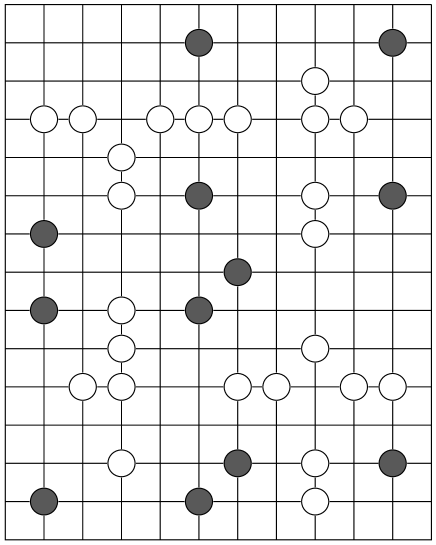
Figure 3: An example of a partially stuck configuration of the DRD model in two dimensions. The particles denoted by black circles are completely immobile, and cannot move under the DRD rules. The mobile particles ( denoted by white circles)can do so only along some horizontal or vertical lines.

There are some straightforward but interesting generalizations of the model. Consider a general exclusion process with $k$ types of particles. In this general model, if we assume that some types of particles cannot exchange positions (setting their exchange rate to zero), their relative order will be conserved and this can be coded in terms of the conservation of an IS. As a simple example, consider a model with 4 species of particles labelled A,B, C and D respectively with the allowed exchanges with equal rates

$$\begin{array}[]{l}AC\rightleftharpoons CA,\;\;\;AD\rightleftharpoons DA\\ BC\rightleftharpoons CB\;\;\;BD\rightleftharpoons DB.\end{array}$$ (43)

This model again has the MSD property. It is easy to see that there are now two irreducible strings which are conserved by the dynamics. This is because the dynamics conserves the relative order of A and B type particles, and also of C and D type particles. In a string specifying the configuration formed of letters A,B,C and D, deleting all occurrences of A and B gives rise to an IS specifying the relative order between C and D type particles, which is a constant of motion. Similarly, deleting all occurrences of C and D characters, we get another independent IS which is also a constant of motion. In a specific sector, where both irreducible strings are known, the dynamics treats A and B particles as indistinguishable, as also C and D. Thus the dynamics is the same as that of the simple exclusion process (with only two species of particles), and is equivalent to the exactly solved Heisenberg model.

The DRD model is interesting in higher dimensions also . For example, it is easy to see that on a square lattice in two dimensions, the number of totally jammed configurations increases exponentially with the number of sites in the system. All configurations with no two adjacent 1’s are totally jammed. These are just the configurations of the hard-square lattice gas model[25], whose number is known to increase exponentially with the area of the system. One can also construct configurations in which almost all sites are jammed, except for a finite number of diffusing dimers, which move along a finite set of horizontal or vertical lines (see fig. 3). Thus the number of sectors in which only some of the particles are moving also increases as exponential of the volume of the system. However, there is no equivalence to the 2-d Heisenberg model, and no obvious analog of the IS to label the disjoint sectors, and solving for the dynamics seems quite difficult.

An interesting generalization of the model would be to the case when the hamiltonian is non-trivial, say an Ising model with nearest or nearest and next-nearest neighbor couplings. Then the allowed processes are assumed to be same as in the simple DRD model discussed above, but the rates are assumed to satisfy detailed balance. In this case, in the steady state, realtive weights of different configurations are given by the Boltzmann weights, and one can determine the pico-canonical partition functions as functions of parameters like temperature in any given sector. The relative weights of different sectors in the sector-averaging define another temperature parameter in the system. This may be identified as the temperature at which freezing occurs( quenching temperature). Details will be discussed in a future publication.

Another generalization of the model would be to make the diffusion asymmetric. The corresponding 3-species exclusion process then becomes asymmetric, and belongs to the KPZ universality class[26]. The invariance of dynamics under exchanging B and C type particles DD again reduces the problem to a simple asymmetric exclusion process of 2 species, known to be exactly soluble by Bethe ansatz techniques [27, 28, 29], and has a non-classical dynamical exponent 3/2. The correlation function of the asymmetric DRD model would map to somewhat complicated multispin correlation functions of the simple asymmetric exclusion process. How these would vary from sector to sector has not been studied so far.

One intriguing feature of this model ( and other models with conserved IS) is the fact that we are able to get an infinity of classical constants of motion by constructing a one parameter family of matrices which commute with each other and with the Hamiltonian. A similar construction is used in integrable models, involving the R-matrix which is assumed to satisfy the Yang -Baxter equation. The similarity of construction suggests that one can devise a more general R-matrix from which both the classical and quantum mechanical conserved quantities are deducible. Such a structure remains to be found.

Acknowledgements: It is a pleasure to thank M. Barma, H. M. Koduvely and G. I. Menon for many useful discussions, and A. Dhar for help in preparation of the manuscript.

References

References

- [1] R. P. Feynman, in Statistical Mechanics: A Set of Lectures (Addison Wesley, Reading, 1990), p1.
- [2] G. I. Menon, M. Barma and D. Dhar, J. Stat. Phys. (1997), to appear.
- [3] See for example, K. Binder and A. P. Young, Rev. Mod. Phys. 58 (1986) 801; M. Mezard, G. Parisi and M. Virasoro in Spin Glass Theory and Beyond,( World Scientific, Singapore, 1988); H. Rieger in Annual Reviews of Computational Physics II, Ed. D. Stauffer (1995) p295; E. Vincent, J. Hammann, M. Ocio, J. P. Beauchaud and L.F. Cugliandolo, preprint (1996) [ condmat 9607224].
- [4] The words ‘microcanonical’ and ‘canonical’ have been used here in a somewhat more general sense than in conventional statistical mechanics textbooks. We use the former to mean the case when the partition function is an integral over phase space, with some product of delta functions as integrand. In the latter case, the integrand is of the form , where are some observables, and are some parameters.
- [5] J. von Neumann, Ann. Math, 32 (1931) 191;
- [6] S. Wiegert, Physica D 56 (1992) 107;
- [7] D. Dhar and M. Barma, Pramana J. Phys.,bf 41 (1993) L193.
- [8] M. Barma and D. Dhar, Phys. Rev. Lett. 73 (1994) 2135.
- [9] M. K. Hari Menon and D. Dhar, J. Phys. A 28, (1995) 6517.
- [10] M. K. Hari Menon, Ph. D. thesis, Bombay University, (1995).
- [11] C. Boldrighini,G. Cosimi, S. Frigio and M. Grasso Nunes, J. Stat. Phys.,55,(1989) 611.
- [12] B. Derrida, S. Janowsky, J. L. Lebowitz and E. R. Speer, J. Stat. Phys.73 (1993) 813.
- [13] P. A. Ferrari, L. R. G. Fontes and Y. Kohayakawa., J. Stat. Phys. 76 (1994) 1153.
- [14] F. C. Alcaraz, M. Droz, M. Henkel and V. Rittenberg, Annals. of Phy. 230: 250, (1994).
- [15] R. Z. Bariev, J. Phys. A 24 L-549-533 (1991).
- [16] J. E. Hirsch, Phys. Lett. A 134, 451 (1989); Physica 158 C 326 (1989).
- [17] See, for example, the article by L. A. Takhtajan in Exactly Solvable Problems in Condensed Matter and Relativistic Field Theory, B. S. Shastry, S. S. Jha and V. Singh, eds. (Springer-Verlag, Berlin, 1986) pp. 175-219.
- [18] S. N. Majumdar and M. Barma, Physica A 177: 366 (1991).
- [19] M. Barma, in Nonequilibrium Statistical Mechanics in One Dimension, V. Privman ed., (Cambridge University Press, to appear).
- [20] M. Barma and D. Dhar, in Proceedings of the International Colloqium on Modern Quantum Field Theory II, S.R. Das, G. Mandal, S. Mukhi and S.R. Wadia eds., (World Scientific, Singapore, 1995), p. 123.
- [21] R. Arratia, Z. Ann. Probab., 11 (1983) 362; T. M. Liggett, Interacting Particle Systems, (Springer, New York, 1985).
- [22] M. Barma, M. D. Grynberg and R. B. Stinchcombe, Phys. Rev. Lett 70: 1033 (1993).
- [23] R. B. Stinchcombe, M. D. Grynberg and M. Barma, Phys. Rev. E 47 : 4018 (1993).
- [24] M. Barma and D. Dhar, in Proceedings of the 19th IUPAP International Conference on Statistical Physics, Xiamen, China, July 31 - Aug 4, 1995, (World Scientific, to appear).
- [25] R. J. Baxter, T. G. Enting and S. K. Tsang, J. Stat. Phys. 22 : 465, (1980).
- [26] M. Kardar, G. Parisi and Y-C. Zhang, Phys. Rev. Lett 56 : 889, (1986).
- [27] D. Dhar, Phase Transitions 9 : 51, (1987); L-H. Gwa and H. Spohn, Phys. Rev. A 46 : 844, (1992).
- [28] T. Halpin-Healy and Y-C. Zhang, Phys. Rep. 254 : 215, (1995).
- [29] D. Kim, Phys. Rev. E 52 : 3512, (1995).