Superconducting properties of the attractive Hubbard model

Abstract

A self-consistent set of equations for the one-electron self-energy in the ladder approximation is derived for the attractive Hubbard model in the superconducting state. The equations provide an extension of a $T$-matrix formalism recently used to study the effect of electron correlations on normal-state properties. An approximation to the set of equations is solved numerically in the intermediate coupling regime, and the one-particle spectral functions are found to have four peaks. This feature is traced back to a peak in the self-energy, which is related to the formation of real-space bound states. For comparison we extend the moment approach to the superconducting state and discuss the crossover from the weak (BCS) to the intermediate coupling regime from the perspective of single-particle spectral densities.

I Introduction

High-temperature superconductors display a wide range of behavior atypical of standard band-theory metals. In the superconducting state these materials become extreme type II superconductors, with a very short coherence volume, which one might take as an indication of tightly bound pairs. Particularly interesting in this respect are recent experiments showing a pseudo-gap structure in the normal-state density-of-states of underdoped Bi₂Sr₂CaCu₂O_8+δ that persists almost up to room temperature [1, 2]. These features suggest that correlation effects strongly affect the properties of such materials. One of the simplest models featuring superconductivity and allowing a systematic study of the effect of electron correlations is the attractive Hubbard model. Although this model is unlikely to provide a microscopic description of high-temperature superconductivity, it is likely that it reveals the effect of correlations on measurable properties.

In a previous work, the effect of electron correlations on some normal-state properties of the attractive Hubbard model was studied using a self-consistent $T$-matrix formalism, going beyond simple mean-field treatments [3]. It was found that for intermediate coupling strengths the attractive interaction gives rise to large momentum real-space bound states with energies below the two-particle continuum and with a pronounced effect on the spectral properties, namely a splitting of the free band into two, one of them associated with virtual bound states. Also, a bending in the static spin-susceptibility was observed for temperatures just above the phase transition.

Thus, it is of significant interest to study the effect of these bound states also in the superconducting state. To this end we derive, in Appendix A, a set of equations for the electron self-energies in the ladder approximation including anomalous diagrams. This is done in a general fashion using the technique of functional derivatives, well-known from the textbook by Kadanoff and Baym [4]. To facilitate a numerical analysis, the anomalous part of the equations is approximated in a somewhat simpler form, which is a reasonable approximation for the parameters of interest. These equations reduce to the familiar $T$-matrix equation in the normal state and provide an obvious extension of the work embarked on in Ref. [3]. In Sec. II we present a numerical solution using the fast Fourier transform (FFT) technique and discuss the physical meaning of the results.

To gain further insight into the electronic properties of the superconducting state we compare the results with a generalization of the moment approach, allowing a description of the diagonal and off-diagonal single-particle spectral function in the superconducting state, concentrating on the weak and intermediate coupling regimes. This formalism is developed in Appendix B, and a comparison is presented in Sec. III.

Our main results include (i) the appearance of four excitation branches in the one-particle spectral function, with symmetric dispersions around the chemical potential, and (ii) that the low-energy behavior with respect to the chemical potential is in qualitative agreement with BCS, whereas the high-energy features are not accounted for in BCS.

II $T$-matrix equations below $T_{\rm c}$

The Hubbard Hamiltonian is defined as

$$H=-t\sum_{<ll^{\prime}>\sigma}c_{l\sigma}^{\dagger}c_{l^{\prime}\sigma}+U\sum_{l}n_{l\uparrow}n_{l\downarrow}-\mu\sum_{l\sigma}n_{l\sigma}\;\;\;,$$ (1)

where $c_{l\sigma}^{\dagger}$($c_{l\sigma}$) are creation (annihilation) electron operators with spin $\sigma$. The number operator is $n_{l\sigma}\equiv c_{l\sigma}^{\dagger}c_{l\sigma}$, $t$ a hopping matrix element between nearest neighbors $l$ and $l^{\prime}$, $U$ the on-site interaction, and $\mu$ the chemical potential in the grand canonical ensemble. Here we consider an attractive interaction, $U<0$. For a review of the attractive Hubbard model, see Micnas et al. [5].

In Appendix A we used functional derivatives to derive self-consistent equations for the self-energy in the ladder approximation in the superconducting state. Here we present a numerical solution of a simplified form of the derived equations, where the superconducting order parameter is only taken into account to lowest order — appropriate when it is significantly less than the bandwidth. The use of a ladder approximation means that only two-particle scattering events are described and restricts the validity of the scheme to dilute systems. Thus, we approximated the self-energy by [6, 7]

$$\Sigma(x,x^{\prime})=\left(\begin{array}[]{cc}G_{22}(x,x^{\prime})T(x^{\prime},x)&\Delta(x)\delta(x-x^{\prime})\\ \Delta^{*}(x)\delta(x-x^{\prime})&G_{11}(x,x^{\prime})T(x^{\prime},x)\end{array}\right)\;\;\;,$$ (2)

where $x=(l,\tau)$ denotes a space-time coordinate and the $T$-matrix in Fourier–Matsubara space is given by

$$T(q,i\varepsilon_{m})=\frac{U}{1-U\chi(q,i\varepsilon_{m})}$$ (3)

with

$$\chi(q,i\varepsilon_{m})\equiv\frac{1}{N\beta}\sum_{k,i\omega_{n}}G_{22}(k-q,i\omega_{n}-i\varepsilon_{m})G_{11}(k,i\omega_{n})\;\;\;,$$ (4)

where $i\varepsilon_{m}$ and $i\omega_{n}$ are bosonic and fermionic Matsubara frequencies, respectively. Another approximation approach, taking the order parameter into account in a higher order than here, can be found in Ref. [8].

In this formalism the two-particle Green’s function, which is also the local-pair propagator, is given by [3]

$$G_{2}({\bf k},i\varepsilon_{n})=\frac{T({\bf k},i\varepsilon_{n})\chi({\bf k},i\varepsilon_{n})}{U}\;\;\;.$$ (5)

Green’s functions are determined self-consistently using Dyson’s equation, Eq. (A2), and the order parameter is determined by $\Delta(x)=UG_{12}(x^{+},x)$. Technical aspects of the numerical solutions using the FFT technique have been described in detail in Ref. [3].

The numerical simulations were performed in two dimensions (2D) for $U/t=-6$, a density of $\rho=0.1$ and a temperature of $T/t=0.05$, which is far below the transition temperature. Here one must note that, owing to the Mermin–Wagner theorem, no phase transition is expected in 2D in systems with a continuous symmetry, and the formalism employed is too simple to describe a Kosterlitz–Thouless phase transition. Nonetheless, it is observed that the formalism does yield a phase transition, in agreement with the results above the transition temperature, where a divergence of the $T$-matrix was observed with decreasing temperature.

In Fig. 1, we present the diagonal one-particle spectral function, $A({\bf k},\omega)$, defined by

$$A({\bf k},\omega)\equiv\lim_{\delta\rightarrow O^{+}}-\frac{1}{\pi}Im[G_{11}({\bf k},\omega+i\delta)],$$ (6)

We see that four peaks exist for every momentum along the diagonal of the Brillouin zone, a situation we will examine in a moment. The value of the order parameter is $\Delta/t=1.04$, which is within the region of validity of the approximation, Eqs. (A31)–(A40). The transition temperature can be found as the temperature where $\Delta$ vanishes and is $T_{\rm c}/t=0.2$, compared to the BCS transition temperature $T_{\rm c}^{\rm BCS}/t=0.66$. The zero-temperature order parameter, critical temperature ratio is now $2\Delta(T=0)/k_{\rm B}T_{\rm c}=10.4$, quite different from the canonical BCS result of $2\Delta(T=0)/k_{\rm B}T_{\rm c}=3.52$.

In Fig. 2, we present the off-diagonal one-particle spectral function, $B({\bf k},\omega)$, which is defined as

$$B({\bf k},\omega)\equiv\lim_{\delta\rightarrow O^{+}}-\frac{1}{\pi}{\rm Im}[G_{12}({\bf k},\omega+i\delta)]\;\;\;.$$ (7)

We also observe four peaks in the off-diagonal one-particle spectral function which are at the same positions as the ones of the diagonal one-particle spectral function. In Sec. III we will see that symmetric poles around the chemical potential are a consequence of Dyson’s equation [Eq. (A3)].

To explain the occurrence of these four peaks in the one-particle spectral functions, let us study the real part of the self-energy. This is presented in Fig. 3. Examining the one-particle Green’s function, $G({\bf k},i\omega_{n})$, coming from Dyson’s equation, we find it is given by [see Eq. (A3)]

$$G({\bf k},z)=\frac{z+\varepsilon_{\bf k}+\Sigma({\bf k},-z)}{(z-\varepsilon_{\bf k}-\Sigma({\bf k},z))(z+\varepsilon_{\bf k}+\Sigma({\bf k},-z))-|\Delta(T)|^{2}}\;\;\;$$ (8)

using $\Sigma_{22}({\bf k},z)=-\Sigma_{11}({\bf k},-z)$. We wish to study the roots of the denominator of Eq. (8). For example, in the BCS case where the self-energies are zero, we obtain two solutions at $\omega=\pm\sqrt{\varepsilon_{\bf k}^{2}+|\Delta(T)|^{2}}$. For ${\bf k}=(\pi,\pi)$, we obtain $\varepsilon_{\bf k}/t\approx 8.4$ because $\varepsilon_{\bf k}$ is measured with respect to the chemical potential, which in our case is $-4.438$ (see Fig. 1). Then, the two roots are located at $\approx\pm 8.5$. These two roots are going to remain for the interacting case, as we will see shortly. The positions of the poles are determined mainly by the real part of the self-energy, and the imaginary part contributes essentially only an additional lifetime effect. Thus, we assume for simplicity that the imaginary part is zero. We then have to find the roots of the equation

$$(\omega-\varepsilon_{\bf k}-\Sigma^{\prime}({\bf k},\omega))(\omega+\varepsilon_{\bf k}+\Sigma^{\prime}({\bf k},-\omega))-|\Delta(T)|^{2}=0\;\;\;,$$ (9)

where $\Sigma^{\prime}({\bf k},\omega)$ is the real part of the self-energy. A rough estimate of the roots at ${\bf k}=(\pi,\pi)$ of Eq. (9) yields the values $\omega/t\approx\pm$2.6, $\pm$8.5. We see that the two previous (i.e. BCS) solutions remain and that there are two other solutions symmetric around the chemical potential. These excitations correspond to electrons bound into local pairs.

Figure 4 shows the imaginary part of the two-particle Green’s function, $-{\rm Im}G_{2}({\bf q},\omega)$. We observe that for zero momentum we find the Cooper resonance, i.e., two symmetric peaks around the chemical potential. However, the Cooper resonance is different above and below $T_{\rm c}$. Above the critical temperature the Cooper resonance is sharp and close to the chemical potential, whereas in the superconducting state the resonance is less sharp and the two peaks are separated by an energy of $\approx 2\Delta$. For larger momenta, we find a peak that yields a narrow band (around $\omega\approx-2\mu+U$). This narrow band is associated with pair states, which is a feature also observed in the $T$-matrix calculations above $T_{\rm c}$ [3]. The pair states give rise to a narrow band in the self-energy, which in turn gives rise to a band of bound electrons in the single-particle excitation spectrum. For this value of the interaction, the band crosses that of the BCS quasiparticles, causing a hybridization and correspondingly a split into four excitation branches.

III Moment approach

To further the understanding of the results, we have generalized the moment approach[9] to the superconducting case. The formalism is derived in Appendix B, and here we present numerical results and compare them with the $T$-matrix results from above.

For the $T$-matrix formalism, we presented numerical data for $U/t=6$ above. This interaction strength was chosen because it provides a clear picture of the essential physics. Unfortunately, the moment approach has a limitation for higher coupling strength, as will be discussed below, and we found it necessary to restrict the coupling strength to $U/t=4$ in the following.

In Figs. 5 and 6 we show the dispersion of the quasiparticles and their weights in the normal state for $U/t=4,\rho=0.1$ in 2D. It can be seen that the attractive interaction splits the free quasiparticle band into two bands. Examining the weights, we identify the unpaired electrons as being the species of electrons with dominating weights — residing in the lower band for low momenta and in the upper band for large momenta. With increasing $U$ the bands separate more, and for some critical $U$ only paired electron reside in the lower band, whereas only unbound electron reside in the upper one [10]. Retaining this set of parameters for the moment, we calculated the dispersion of the quasiparticles and their weights in the superconducting state using the moment approach outlined in Appendix B.

The results for $U/t=4,\rho=0.1$ are shown in Figs. 7 and 8. We obtain four bands instead of two in the normal state, with a gap around the chemical potential. The lowest band has negligible weight (Fig. 8) and is irrelevant for the diagonal spectral function, although it makes a finite contribution to the off-diagonal spectral function and thereby to the gap equation and $T_{\rm c}$. An essential point is that the band wherein the chemical potential was located as well as the weight are divided into two, leaving the upper band practically unchanged. For this reason, a BCS treatment still describes the behavior around the chemical potential reasonably well, but misses the additional excitation branches. These affect the off-diagonal Green’s function and hence the gap equation, Eq. (B38). Indeed, the BCS transition temperature $T_{\rm c}^{\rm BCS}/t=0.37$ is reduced to $T_{\rm c}/t=0.19$. Thus, whereas the BCS transition temperature increased without bounds with increasing coupling strength, the real transition temperature is reduced compared to that resulting from the increasing pair mass. Indeed, for infinite coupling strength all pairs would be localized and the transition temperature would go to zero. These features characterize the crossover from weak to intermediate coupling. In Figs. 7 and 8 we have also included results from numerical $T$-matrix calculations for the same coupling strength and find quite a good overall fit. The discrepancy in the dispersion for large momenta is also found in the normal state and can be attributed to the neglect of the $k$-dependence in the approximation for the band-correction term in Eq. (B19).

For increasing $U$ we find that the chemical potential moves into the correlation gap and that the model becomes an insulator. The formalism used here yields $T_{\rm c}=0$, which is correct in the sense that we no longer expect a Fermi-surface instability for large $U$. Instead we expect to have a scenario of Bose–Einstein condensation of preformed pairs, yielding a finite transition temperature. The description of this phenomenon is beyond the current formulation, however. Considering that the moments describe the transition to the strong-coupling regime well in the normal state, we expect that this will also be so would we satisfy more off-diagonal moments. For instance in our approach all odd off-diagonal moments are zero. This, however, is not true for the exact moments. We thus believe that these nonzero moments must be satisfied in order to describe the crossover to Bose–Einstein condensation.

IV Conclusions

Using a functional derivative technique, we have generalized the particle–particle ladder approximation to the superconducting state, providing an obvious extension of previous work in the normal state. The resulting gap equation is a complicated, nonlinear integral equation, whose solution is difficult to obtain. Recently, Bickers and White evaluated the $T$-matrix eigenvalues, which is equivalent to looking for normal-state instabilities that signal second-order phase transitions [11]. In contrast, the equations derived here cover the entire range of temperature, both above and below $T_{\rm c}$.

Another calculation was carried out by Haussmann [12], who developed a perturbative formalism for the vertex function starting from diagrammatic techniques, including both particle–particle and particle–hole channels in the Bethe–Salpeter equation. He ultimately neglects the particle–hole channel, the vertex function is transformed to the scattering $T$-matrix, and he treats superconductivity in a mean-field fashion. Thus, no direct comparison with our equations is possible.

A somewhat simplified version of the equations derived here has been solved numerically using the FFT technique. The main result is the appearance of four peaks in both the diagonal and off-diagonal one-particle spectral functions, which can be explained by a narrow band in the self-energy, related to the formation of real-space bound states below the two-particle continuum.

We presented an extension of the moment approach to the superconducting state, providing an approximate expression of the single-particle spectral density. Although lifetime effects are neglected and correlations effects in the band-correction term have been treated approximately, our approach provides new insight into the crossover from the weak to the intermediate coupling regimes.

For the specific case of $U/t=4,\rho=0.1$, we have shown that the single-particle spectrum in the superconducting state exhibits four symmetric branches with respect to the chemical potential. The low-energy part (with respect to $\mu$) resembles BCS behavior, whereas the high-energy physics is strongly modified. This led to a reduction of $T_{\rm c}$ in comparison with the expectation from BCS.

Acknowlegdments

We thank the Swiss National Foundation for financial support under project No. 21-31096-91 (Theory of Layered Superconductors). One of the authors (JJRN) acknowledges partial support from the Brazilian Agency CNPq (project no. 300705/95-6) and from CONICIT (project no. F-139). This work was carried out at IBM Rüschlikon and its kind hospitality is fully appreciated. We thank R. Micnas and J. M. Singer for useful discussions.

A Derivation of $T$-matrix equations

It is convenient to define the Nambu–Green function

$${\cal G}(l\tau,l^{\prime}\tau^{\prime})=\left(\begin{array}[]{cc}-\langle T_{\tau}c_{l\uparrow}(\tau)c_{l^{\prime}\uparrow}^{\dagger}(\tau^{\prime})\rangle&\langle T_{\tau}c_{l\uparrow}(\tau)c_{l^{\prime}\downarrow}(\tau^{\prime})\rangle\\ \langle T_{\tau}c_{l\downarrow}^{\dagger}(\tau)c_{l^{\prime}\uparrow}^{\dagger}(\tau^{\prime})\rangle&\langle T_{\tau}c_{l\downarrow}^{\dagger}(\tau)c_{l^{\prime}\downarrow}(\tau^{\prime})\rangle\end{array}\right)$$ (A1)

where $T_{\tau}$ is the time ordering operator.

The Dyson equation for the self-energies in Fourier–Matsubara space is

$$\left(\begin{array}[]{cc}i\omega_{n}-\varepsilon_{\bf k}-\Sigma_{11}({\bf k},i\omega_{n})&-\Sigma_{12}({\bf k},i\omega_{n})\\ -\Sigma_{21}({\bf k},i\omega_{n})&i\omega_{n}+\varepsilon_{\bf k}-\Sigma_{22}({\bf k},i\omega_{n})\end{array}\right)\left(\begin{array}[]{ll}G_{11}({\bf k},i\omega_{n})&G_{12}({\bf k},i\omega_{n})\\ G_{21}({\bf k},i\omega_{n})&G_{22}({\bf k},i\omega_{n})\end{array}\right)=\left(\begin{array}[]{rr}1&{~{}0}\\ 0&1\end{array}\right)\;\;\;,$$ (A2)

where $i\omega_{n}\equiv\pi(2n+1)/\beta$ are the fermionic Matsubara frequencies and $\beta=1/(k_{\rm B}T)$ the inverse temperature. Formally the components of the Nambu–Green function can then be expressed as

$$G_{11}({\bf k},i\omega_{n}) = -G_{22}({\bf k},-i\omega_{n})=\frac{i\omega_{n}+\varepsilon_{\bf k}-\Sigma_{22}({\bf k},i\omega_{n})}{(i\omega_{n}-\varepsilon_{\bf k}-\Sigma_{11}({\bf k},i\omega_{n}))(i\omega_{n}+\varepsilon_{\bf k}-\Sigma_{22}({\bf k},i\omega_{n}))-\Sigma_{12}({\bf k},i\omega_{n})\Sigma_{21}({\bf k},i\omega_{n})}~{},$$ (A3)

$$G_{12}({\bf k},i\omega_{n}) = G_{21}({\bf k},-i\omega_{n})=\frac{\Sigma_{12}({\bf k},i\omega_{n})}{(i\omega_{n}-\varepsilon_{\bf k}-\Sigma_{11}({\bf k},i\omega_{n}))(i\omega_{n}+\varepsilon_{\bf k}-\Sigma_{22}({\bf k},i\omega_{n}))-\Sigma_{12}({\bf k},i\omega_{n})\Sigma_{21}({\bf k},i\omega_{n})}\;\;\;,$$ (A4)

where the $d$-dimensional dispersion is given by $\varepsilon_{\bf k}=-2t\sum_{\alpha}\cos(k_{\alpha}a_{\alpha})-\mu$. The problem of calculating the components of the one-particle Nambu–Green function is then translated to the evaluation of the self-energies [13].

The equation of motion for the Nambu–Green function contains four-point correlation functions that cannot be evaluated analytically. In order to derive a perturbation expansion we add auxiliary source fields to the Hamiltonian

$$H_{\rm S}=\sum_{l}\left(\rho_{l}^{*}c_{l\downarrow}^{\dagger}c_{l\uparrow}^{\dagger}+\rho_{l}c_{l\uparrow}c_{l\downarrow}\right)$$ (A5)

and ultimately take the limit of these fields going to zero. This particular way of generating four-point correlation functions leads in the following to expressions for particle–particle scattering, which in turn leads to superconductivity in the Cooper channel. It is important to note that this approach does not generate particle–hole diagrams.

The four-point correlation functions can now be written in terms of derivatives with respect to the auxiliary fields, and the equation of motion can be written

$$\left(\begin{array}[]{ll}~{}~{}~{}~{}~{}~{}~{}-\frac{\delta}{\delta\tau}+t_{ll^{\prime}}+\mu&\Delta(x)\delta(x-x^{\prime})+U\frac{\delta}{\delta\rho(x)}-\rho^{*}(x)\\ \Delta^{*}(x)\delta(x-x^{\prime})+U\frac{\delta}{\delta\rho^{*}(x)}+\rho(x)&~{}~{}~{}~{}~{}~{}~{}~{}\frac{\delta}{\delta\tau}+t_{ll^{\prime}}+\mu\end{array}\right){\cal G}(x,x^{\prime})=\left(\begin{array}[]{rr}1&{~{}0}\\ 0&1\end{array}\right)\delta(x-x^{\prime})\;\;\;,$$ (A10)

where $\Delta(x)=UG_{12}(x^{+},x)$ and $\Delta^{*}(x)=UG_{21}(x^{+},x)$. Here and in the following, we use the shorthand notation $x=(l,\tau)$ for a space-time coordinate. Then, from Eq.  (A10), the self-energy is given by $\Sigma(x,x^{\prime})=\Sigma^{0}(x,x^{\prime})+\Sigma^{1}(x,x^{\prime})$, where

$$\Sigma^{0}(x,x^{\prime})=\left(\begin{array}[]{cc}0&\Delta(x)-\rho^{*}(x)\\ \Delta^{*}(x)-\rho(x)&0\end{array}\right)\delta(x-x^{\prime})$$ (A11)

and

$$\Sigma^{1}(x,\overline{a}){\cal G}(\overline{a},x^{\prime})=U\left(\begin{array}[]{cc}0&\frac{\delta}{\delta\rho(x)}\\ \frac{\delta}{\delta\rho^{*}(x)}&0\end{array}\right){\cal G}(x,x^{\prime})\;\;\;,$$ (A12)

where we used the notation $f(\overline{a})g(\overline{a})\equiv\int daf(a)g(a)$. In the following, we also use the usual identity $\delta{\cal G}(x,x^{\prime})={\cal G}(x,\overline{a})\delta\Sigma(\overline{a},\overline{b}){\cal G}(\overline{b},x^{\prime})$ [4].

¿From Eq. (A12) we find

$$\Sigma^{1}(x,x^{\prime})=U\sum_{s=1}^{2}M_{s}{\cal G}(x,\overline{a})\frac{\delta\Sigma(\overline{a},x^{\prime})}{\delta\rho_{s}(x)}\;\;\;,$$ (A13)

where the matrices $M_{1(2)}$ are defined as

$$M_{1}=\left(\begin{array}[]{cc}0&1\\ 0&0\end{array}\right)\;\;\;;\;\;\;M_{2}=\left(\begin{array}[]{rr}0&0\\ 1&0\end{array}\right)$$ (A14)

and $\rho_{1}(x)=\rho(x),\rho_{2}(x)=\rho^{*}(x)$.

We now introduce a vertex function

$${\mit\Gamma}^{(s)}(x,x^{\prime}|y)\equiv U\frac{\delta\Sigma(x,x^{\prime})}{\delta\rho_{s}(y)}\;\;\;,$$ (A15)

which obeys the equation

$${\mit\Gamma}^{(s)}(x,x^{\prime}|y) = -U\delta(x-x^{\prime})\delta(x-y)M_{s}^{\rm T}$$ (A16)

$$+ U\delta(x-x^{\prime})\left[{\cal G}(x,\overline{a}){\mit\Gamma}^{(s)}(\overline{a},\overline{b}|y){\cal G}(\overline{b},x^{\prime})\right]_{\rm off}$$ (A17)

$$+ \sum_{s^{\prime}}M_{s^{\prime}}{\cal G}(x,\overline{a}){\mit\Gamma}^{(s)}(\overline{a},\overline{b}|y){\cal G}(\overline{b},\overline{c}){\mit\Gamma}^{(s^{\prime})}(\overline{c},x^{\prime}|x)$$ (A18)

$$+ U\sum_{s^{\prime}}{\cal G}(x,\overline{a})\frac{\delta{\mit\Gamma}^{(s^{\prime})}(\overline{a},x^{\prime}|x)}{\delta\rho_{s}(y)}\;\;\;,$$ (A19)

where $[...]_{\rm off}$ denotes the $2\times 2$ matrix with zero diagonal elements and off-diagonal elements given by the matrix enclosed in brackets, and $M^{\rm T}$ is the transpose of the matrix $M$. The self-energy is given by

$$\Sigma(x,x)=\Sigma^{0}(x,x^{\prime})+\sum_{s}{\cal G}(x,\overline{a}){\mit\Gamma}^{(s)}(\overline{a},x^{\prime}|x)\;\;\;.$$ (A20)

As Eq. (A16) is not practically manageable, we wish to approximate it to a simpler form taking only ladder diagrams into account, which describes repeated scattering between two particles. This contribution is expected to dominate for small densities. A graphical analysis will easily show that the latter term in Eq. (A16) corresponds to higher-order diagrams, so we omit it. The eight matrix elements of the vertex function then read

$${\mit\Gamma}^{(s)}_{11}(x,x^{\prime}|y) = G_{2\alpha}(x,\overline{a}){\mit\Gamma}^{(s)}_{\alpha\beta}(\overline{a},\overline{b}|y)G_{\beta\gamma}(\overline{b},\overline{c}){\mit\Gamma}^{(1)}_{\gamma 1}(\overline{c},x^{\prime}|x)\;\;\;,$$ (A21)

$${\mit\Gamma}^{(1)}_{12}(x,x^{\prime}|y) = U\delta(x-x^{\prime})G_{1\alpha}(x,\overline{a}){\mit\Gamma}^{(1)}_{\alpha\beta}(\overline{a},\overline{b}|y)G_{\beta 2}(\overline{b},x^{\prime})+G_{2\alpha}(x,\overline{a}){\mit\Gamma}^{(1)}_{\alpha\beta}(\overline{a},\overline{b}|y)G_{\beta\gamma}(\overline{b},\overline{c}){\mit\Gamma}^{(1)}_{\gamma 2}(\overline{c},x^{\prime}|x)\;\;\;,$$ (A22)

$${\mit\Gamma}^{(1)}_{21}(x,x^{\prime}|y) = -U\delta(x-x^{\prime})\delta(x-y)+U\delta(x-x^{\prime})G_{2\alpha}(x,\overline{a}){\mit\Gamma}^{(1)}_{\alpha\beta}(\overline{a},\overline{b}|y)G_{\beta 1}(\overline{b},x^{\prime})$$ (A24)

$$+G_{1\alpha}(x,\overline{a}){\mit\Gamma}^{(1)}_{\alpha\beta}(\overline{a},\overline{b}|y)G_{\beta\gamma}(\overline{b},\overline{c}){\mit\Gamma}^{(2)}_{\gamma 1}(\overline{c},x^{\prime}|x)\;\;\;,$$

$${\mit\Gamma}^{(s)}_{22}(x,x^{\prime}|y) = G_{1\alpha}(x,\overline{a}){\mit\Gamma}^{(s)}_{\alpha\beta}(\overline{a},\overline{b}|y)G_{\beta\gamma}(\overline{b},\overline{c}){\mit\Gamma}^{(2)}_{\gamma 2}(\overline{c},x^{\prime}|x)\;\;\;,$$ (A25)

$${\mit\Gamma}^{(2)}_{12}(x,x^{\prime}|y) = -U\delta(x-x^{\prime})\delta(x-y)+U\delta(x-x^{\prime})G_{1\alpha}(x,\overline{a}){\mit\Gamma}^{(2)}_{\alpha\beta}(\overline{a},\overline{b}|y)G_{\beta 2}(\overline{b},x^{\prime})$$ (A27)

$$+G_{2\alpha}(x,\overline{a}){\mit\Gamma}^{(2)}_{\alpha\beta}(\overline{a},\overline{b}|y)G_{\beta\gamma}(\overline{b},\overline{c}){\mit\Gamma}^{(1)}_{\gamma 2}(\overline{c},x^{\prime}|x)\;\;\;,$$

$${\mit\Gamma}^{(2)}_{21}(x,x^{\prime}|y) = U\delta(x-x^{\prime})G_{2\alpha}(x,\overline{a}){\mit\Gamma}^{(2)}_{\alpha\beta}(\overline{a},\overline{b}|y)G_{\beta 1}(\overline{b},x^{\prime})+G_{1\alpha}(x,\overline{a}){\mit\Gamma}^{(2)}_{\alpha\beta}(\overline{a},\overline{b}|y)G_{\beta\gamma}(\overline{b},\overline{c}){\mit\Gamma}^{(2)}_{\gamma 1}(\overline{c},x^{\prime}|x)\;\;\;,$$ (A28)

where summation on repeated indices is understood. Similarly, the correction to the self-energy, $\Sigma^{1}$, is given by

$$\Sigma^{1}_{1\alpha}(x,x^{\prime}) = G_{21}(x,\overline{a}){\mit\Gamma}^{(1)}_{1\alpha}(\overline{a},x^{\prime}|x)+G_{22}(x,\overline{a}){\mit\Gamma}^{(1)}_{2\alpha}(\overline{a},x^{\prime}|x)\;\;\;,$$ (A29)

$$\Sigma^{1}_{2\alpha}(x,x^{\prime}) = G_{11}(x,\overline{a}){\mit\Gamma}^{(2)}_{1\alpha}(\overline{a},x^{\prime}|x)+G_{12}(x,\overline{a}){\mit\Gamma}^{(2)}_{2\alpha}(\overline{a},x^{\prime}|x)\;\;\;.$$ (A30)

To further simplify this set of equations we expand it to second order in the anomalous Green’s functions, $G_{12}(G_{21})$, which yields the following approximate form of the vertex functions

$${\mit\Gamma}^{(s)}_{11}(x,x^{\prime}|y) \approx G_{22}(x,\overline{a}){\mit\Gamma}^{(s)}_{21}(\overline{a},\overline{b}|y)G_{12}(\overline{b},\overline{c}){\mit\Gamma}^{(1)}_{21}(\overline{c},x^{\prime}|x)\;\;\;,$$ (A31)

$${\mit\Gamma}^{(1)}_{12}(x,x^{\prime}|y) \approx U\delta(x-x^{\prime})G_{12}(x,\overline{a}){\mit\Gamma}^{(1)}_{21}(\overline{a},\overline{b}|y)G_{12}(\overline{b},x^{\prime})~{}~{},$$ (A32)

$${\mit\Gamma}^{(1)}_{21}(x,x^{\prime}|y) \approx -U\delta(x-x^{\prime})\delta(x-y)+U\delta(x-x^{\prime})G_{22}(x,\overline{a}){\mit\Gamma}^{(1)}_{21}(\overline{a},\overline{b}|y)G_{11}(\overline{b},x^{\prime})\;\;\;,$$ (A33)

$${\mit\Gamma}^{(s)}_{22}(x,x^{\prime}|y) \approx G_{12}(x,\overline{a}){\mit\Gamma}^{(s)}_{21}(\overline{a},\overline{b}|y)G_{11}(\overline{b},\overline{c}){\mit\Gamma}^{(2)}_{12}(\overline{c},x^{\prime}|x)\;\;\;,$$ (A34)

$${\mit\Gamma}^{(2)}_{12}(x,x^{\prime}|y) \approx -U\delta(x-x^{\prime})\delta(x-y)+U\delta(x-x^{\prime})G_{11}(x,\overline{a}){\mit\Gamma}^{(2)}_{12}(\overline{a},\overline{b}|y)G_{22}(\overline{b},x^{\prime})\;\;\;,$$ (A35)

$${\mit\Gamma}^{(2)}_{21}(x,x^{\prime}|y) \approx U\delta(x-x^{\prime})G_{21}(x,\overline{a}){\mit\Gamma}^{(2)}_{12}(\overline{a},\overline{b}|y)G_{21}(\overline{b},x^{\prime})\;\;\;,$$ (A36)

¿From Eqs. (A31) we conclude that ${\mit\Gamma}^{(1)}_{21}(x,x^{\prime}|y)$ and ${\mit\Gamma}^{(2)}_{12}(x,x^{\prime}|y)$ are related to the $T$-matrix equations above $T_{\rm c}$ [3, 14]

$${\mit\Gamma}^{(1)}_{21}(x,x^{\prime}|y)={\mit\Gamma}^{(2)}_{12}(x,x^{\prime}|y)=-\delta(x-x^{\prime})T(x,y)\;\;\;,$$ (A37)

where $T(x,y)$ in reciprocal space has the form

$$T(q,i\varepsilon_{m})=\frac{U}{1-U\chi(q,i\varepsilon_{m})}$$ (A38)

with

$$\chi(q,i\varepsilon_{m})\equiv\frac{1}{N\beta}\sum_{k,i\omega_{n}}G_{22}(k-q,i\omega_{n}-i\varepsilon_{m})G_{11}(k,i\omega_{n})\;\;\;,$$ (A39)

and $i\varepsilon_{n}\equiv 2\pi n/\beta$ are the bosonic Matsubara frequencies.

Using Eqs. (A37) and (A38), we obtain the self-energies to second order in $G_{12}(G_{21})$:

$$\Sigma^{1}_{11}(x,x^{\prime}) = G_{22}(x,x^{\prime})T(x^{\prime},x)+G_{21}(x,\overline{a})G_{22}(\overline{a},\overline{b})T(\overline{b},x)G_{12}(\overline{b},x^{\prime})T(x^{\prime},x)\;\;\;,$$ (A40)

$$\Sigma^{1}_{12}(x,x^{\prime}) = G_{22}(x,\overline{a})G_{12}(\overline{a},\overline{b})T(\overline{b},x)G_{11}(\overline{b},x^{\prime})T(x^{\prime},\overline{a})\;\;\;,$$ (A41)

$$\Sigma^{1}_{21}(x,x^{\prime}) = G_{11}(x,\overline{a})G_{21}(\overline{a},\overline{b})T(\overline{b},x)G_{22}(\overline{b},x^{\prime})T(x^{\prime},\overline{a})\;\;\;,$$ (A42)

$$\Sigma^{1}_{22}(x,x^{\prime}) = G_{11}(x,x^{\prime})T(x^{\prime},x)+G_{12}(x,\overline{a})G_{11}(\overline{a},\overline{b})T(\overline{b},x)G_{21}(\overline{b},x^{\prime})T(x^{\prime},x)\;\;\;.$$ (A43)

This expansion is valid for $\Delta/W\ll 1$, where $W=2dt$ is the bandwidth.

To solve Eqs. (A3) and (A38)–(A40) one would also have to fix the chemical potential from the particle number using

$$\rho(T,\mu)=\lim_{\eta\rightarrow 0^{+}}\frac{1}{\beta N}\sum_{\omega_{n},{\bf k}}G({\bf k},i\omega_{n})\exp(i\omega_{n}\eta)\;\;\;,$$ (A44)

where $\rho$ is the electron concentration per spin and is defined in the interval $[0,1]$. Thus, the set of Eqs. (A3) and (A38)–(A44) represents a set of nonlinear self-consistent equations, which must be solved numerically.

We note that an expansion of the final equations, Eqs. (A31)–(A40), to first order in $U$ simply yields the well-known BCS expressions. To second order in $U$, the result is identical to that of Martín–Rodero and Flores [15]. The second-order expansion was found to yield the same gap equation as in BCS, but with a renormalized interaction.

B Derivation of moment equations

Introduce the diagonal and off-diagonal one-particle Green’s function

$$G_{\sigma}(i-j,\tau)=-\langle T_{\tau}c_{i\sigma}(\tau)c_{j\sigma}^{\dagger}(0)\rangle$$ (B1)

and

$$F(i-j,\tau)=-\langle T_{\tau}c_{i\uparrow}(\tau)c_{j\downarrow}(0)\rangle\;\;\;,$$ (B2)

where $T_{\tau}$ is the time-ordering operator, as well as the associated spectral functions

$$A(k,\omega) = -\frac{1}{\pi}{\rm Im}G(k,\omega+i\delta)\;\;\;,$$ (B3)

$$B(k,\omega) = -\frac{1}{\pi}{\rm Im}F(k,\omega+i\delta)\;\;\;.$$ (B4)

To construct approximate expressions for the spectral functions, it is useful to consider the frequency moments

$$A_{n}(k) = \int_{-\infty}^{\infty}d\omega\,\omega^{n}A(k,\omega)\;\;\;,$$ (B5)

$$B_{n}(k) = \int_{-\infty}^{\infty}d\omega\,\omega^{n}B(k,\omega)\;\;\;.$$ (B6)

With the $d$-dimensional dispersion defined as

$$\epsilon_{k}=-2t\sum_{i=1}^{d}\cos(k_{i}r_{i})\;\;\;,$$ (B7)

the exact four first diagonal moments are given by[9]

$$A_{0}(k) = 1$$ (B8)

$$A_{1}(k) = a_{1}=\epsilon_{k}-\mu-\rho U$$ (B9)

$$A_{2}(k) = a_{2}=(\epsilon_{k}-\mu)^{2}-2(\epsilon_{k}-\mu)\rho U+\rho U^{2}$$ (B10)

$$A_{3}(k) = a_{3}=(\epsilon_{k}-\mu)^{3}-3(\epsilon_{k}-\mu)\rho U+(\epsilon_{k}-\mu)U^{2}\rho(2+\rho)+(\epsilon_{k}-\mu)\rho^{2}U^{2}$$ (B12)

$$-U^{3}\rho+U^{2}\rho(1-\rho)K(k)\;\;\;,$$

where

$$\rho(1-\rho)K(k) = K+K_{w}(k)$$ (B13)

$$K = \frac{1}{N}\sum_{ij}\langle c_{i\bar{\sigma}}^{\dagger}c_{j\bar{\sigma}}(2n_{i\sigma}-1)\rangle$$ (B14)

$$K_{w}(k) = \frac{1}{N}\sum_{ij}t_{ij}e^{ik(r_{i}-r_{j})}\{\langle n_{i\bar{\sigma}}n_{j\bar{\sigma}}\rangle-\rho^{2}$$ (B15)

$$- \langle c_{j\sigma}^{\dagger}c_{j\bar{\sigma}}^{\dagger}c_{i\bar{\sigma}}c_{i\sigma}\rangle-\langle c_{j\sigma}^{\dagger}c_{i\bar{\sigma}}^{\dagger}c_{j\bar{\sigma}}c_{i\sigma}\rangle\}$$ (B16)

and the first two off-diagonal moments are given by

$$B_{0}(k) = 0$$ (B17)

$$B_{1}(k) = -U\sum_{i}\langle c_{i\downarrow}c_{i\uparrow}\rangle\;\;\;.$$ (B18)

In the normal state the first four frequency moments have recently been used in conjunction with an ansatz of the form $A(k,\omega)=\tilde{\alpha}_{1}(k)\delta(\omega-\tilde{\Omega}_{1}(k))+\tilde{\alpha}_{2}(k)\delta(\omega-\tilde{\Omega}_{2}(k))$. The $k$-dependence in Eq. (B13) is approximated by its momentum average. Only Eq. (B14) contributes to the average and is given by [9]

$$\rho(1-\rho)K = -\frac{1}{N}\sum_{k}\sum_{i}\alpha_{i}(k)\epsilon_{k}n_{f}(\Omega_{i}(k))$$ (B19)

$$\times \left[\frac{2}{U}(\Omega_{i}(k)-\epsilon_{k})+1\right]\;\;\;,$$ (B20)

where $n_{f}(\omega)$ is the Fermi distribution function. The chemical potential is obtained by fixing the density using

$$\rho=\sum_{k,i}\alpha_{i}n_{f}(\Omega_{i}(k))\;\;\;.$$ (B21)

To analyze the superconducting state we make the assumption that the general structure of the diagonal part of the self-energy does not change in the superconducting state. As the diagonal part of the self-energy is related primarily to pair-interaction physics, we expect this to be a reasonable approximation. Thus, we express the self-energy as [3, 10]

$$\frac{1}{z-\epsilon_{k}+\Sigma_{\uparrow}(k,z)}=\frac{\alpha_{1}(k)}{z-\Omega_{1}(k)}+\frac{\alpha_{2}(k)}{z-\Omega_{2}(k)}\;\;\;,$$ (B22)

where $\alpha_{1}(k)$, $\alpha_{2}(k)$, $\Omega_{1}(k)$, $\Omega_{2}(k)$ are functions to be determined. Note that this approximation neglects lifetime effects.

The diagonal and off-diagonal Green’s function in the superconducting state is now given by Dyson’s equation

$$G_{\uparrow}(k,z) = \frac{z+\epsilon_{k}-\Sigma_{\downarrow}(k,z)}{(z-\epsilon_{k}+\Sigma_{\uparrow}(k,z))(z+\epsilon_{k}-\Sigma_{\downarrow}(k,z))-|\Delta_{k}|^{2}}$$ (B23)

$$F(k,z) = \frac{\Delta_{k}}{(z-\epsilon_{k}+\Sigma_{\uparrow}(k,z))(z+\epsilon_{k}+\Sigma_{\downarrow}(k,z))-|\Delta_{k}|^{2}}\;\;\;,$$ (B24)

where $\Sigma_{\downarrow}(k,z)=-\Sigma_{\uparrow}(k,-z)$. In Dyson’s equation we have made the additional assumption that the off-diagonal part of the self-energy, $\Delta_{k}$, is independent of frequency. This assumption is likely to be wrong for large coupling strengths, where $\Delta_{k}$ might contain additional structure related to the existence of local pairs.

Combining the above, we can write Green’s functions for frequencies on the real axis as

$$G_{\uparrow}(k,\omega) = \frac{\alpha_{1}(k)(\omega+\Omega_{1}(k))(\omega^{2}-\Omega_{2}^{2}(k))+\alpha_{2}(k)(\omega+\Omega_{2}(k))(\omega^{2}-\Omega_{1}^{2}(k))}{(\omega^{2}-\omega_{0}^{2}(k))(\omega^{2}-\omega_{1}^{2}(k))}$$ (B25)

$$F(k,\omega) = \frac{\Delta_{k}[\omega^{2}-(\alpha_{1}(k)\Omega_{2}(k)+\alpha_{2}(k)\Omega_{1}(k))^{2}]}{(\omega^{2}-\omega_{0}^{2}(k))(\omega^{2}-\omega_{1}^{2}(k))}\;\;\;,$$ (B26)

where $\pm\omega_{0}(k)$ and $\pm\omega_{1}(k)$ are the dispersions of the resulting four poles given by

$$\omega_{0,1}^{2}(k)=\frac{1}{2}\left(\Delta_{k}^{2}+\Omega_{1}^{2}(k)+\Omega_{2}^{2}(k)\pm\sqrt{[\Delta_{k}^{2}+\Omega_{1}^{2}(k)+\Omega_{2}^{2}(k)]^{2}-4[\Omega_{1}^{2}(k)\Omega_{2}^{2}(k)+\Delta^{2}_{k}(\alpha_{1}(k)\Omega_{2}(k)+\alpha_{2}(k)\Omega_{1}(k))^{2}]}\right)\;\;\;.$$ (B27)

The corresponding spectral functions, Eqs. (B3) and (B4), can then be written as $A(k,\omega)=\tilde{\alpha}_{1}(k)\delta(\omega-\omega_{0})+\tilde{\alpha}_{2}(k)\delta(\omega+\omega_{0})+\tilde{\alpha}_{3}(k)\delta(\omega-\omega_{1})+\tilde{\alpha}_{4}(k)\delta(\omega+\omega_{1})$ and $B(k,\omega)=\beta_{1}(\delta(\omega-\omega_{0})-\delta(\omega+\omega_{0}))+\beta_{2}(\delta(\omega-\omega_{1})-\delta(\omega+\omega_{1}))$. The weights are found as the residues of the poles and given by

$$\tilde{\alpha}_{1}(k) = \frac{\alpha_{1}(k)(\omega_{0}(k)+\Omega_{1}(k))(\omega_{0}(k)^{2}-\Omega_{2}(k)^{2})+\alpha_{2}(k)(\omega_{0}(k)+\Omega_{2}(k))(\omega_{0}(k)^{2}-\Omega_{1}(k)^{2})}{2\omega_{0}(k)(\omega_{0}(k)^{2}-\omega_{1}(k)^{2})}$$ (B28)

$$\tilde{\alpha}_{2}(k) = \frac{\alpha_{1}(k)(-\omega_{0}(k)+\Omega_{1}(k))(\omega_{0}(k)^{2}-\Omega_{2}(k)^{2})+\alpha_{2}(k)(-\omega_{0}(k)+\Omega_{2}(k))(\omega_{0}(k)^{2}-\Omega_{1}(k)^{2})}{-2\omega_{0}(k)(\omega_{0}(k)^{2}-\omega_{1}(k)^{2})}$$ (B29)

$$\tilde{\alpha}_{3}(k) = \frac{\alpha_{1}(k)(\omega_{1}(k)+\Omega_{1}(k))(\omega_{1}(k)^{2}-\Omega_{2}(k)^{2})+\alpha_{2}(k)(\omega_{1}(k)+\Omega_{2}(k))(\omega_{1}(k)^{2}-\Omega_{1}(k)^{2})}{2\omega_{1}(k)(\omega_{1}(k)^{2}-\omega_{0}(k)^{2})}$$ (B30)

$$\tilde{\alpha}_{4}(k) = \frac{\alpha_{1}(k)(-\omega_{1}(k)+\Omega_{1}(k))(\omega_{1}(k)^{2}-\Omega_{2}(k)^{2})+\alpha_{2}(k)(-\omega_{1}(k)+\Omega_{2}(k))(\omega_{1}(k)^{2}-\Omega_{1}(k)^{2})}{-2\omega_{1}(k)(\omega_{1}(k)^{2}-\omega_{0}(k)^{2})}$$ (B31)

$$\tilde{\beta_{1}}(k) = \frac{\Delta_{k}(\omega_{0}(k)^{2}-(\alpha_{1}(k)\Omega_{2}(k)+\alpha_{2}(k)\Omega_{1}(k))^{2})}{2\omega_{0}(k)(\omega_{0}^{2}-\omega_{1}^{2})}$$ (B32)

$$\tilde{\beta_{2}}(k) = \frac{\Delta_{k}(\omega_{0}(k)^{2}-(\alpha_{1}(k)\Omega_{2}(k)+\alpha_{2}(k)\Omega_{1}(k))^{2})}{2\omega_{1}(k)(\omega_{1}^{2}-\omega_{0}^{2})}\;\;\;.$$ (B33)

Knowing the spectral functions, we now insert them into the moment equations (B8)–(B12) and obtain the following for the superconducting state:

$$\alpha_{1}(k)+\alpha_{2}(k) = 1$$ (B34)

$$\alpha_{1}(k)\Omega_{1}(k)+\alpha_{2}(k)\Omega_{2}(k) = a_{1}$$ (B35)

$$\alpha_{1}(k)\Omega_{1}^{2}(k)+\alpha_{2}(k)\Omega_{2}^{2}(k) = a_{2}-\Delta_{k}^{2}$$ (B36)

$$\alpha_{1}(k)\Omega_{1}^{3}(k)+\alpha_{2}(k)\Omega_{2}^{3}(k) = a_{3}-\Delta_{k}^{2}a_{1}\;\;\;.$$ (B37)

The first two off-diagonal moment equations, Eqs. (B17) and (B18), are automatically satisfied by our Dyson’s equation.

The resulting moment equations for the superconducting state can be solved and uniquely determine the form of the spectral functions. The second off-diagonal moment equation yields the gap equation

$$\frac{\Delta_{k}}{U}=\sum_{k}\int_{-\infty}^{\infty}d\omega\,n_{f}(\omega)B(k,\omega)\;\;\;.$$ (B38)

We immediately see that in this approach the order parameter is a constant, $\Delta_{k}=\Delta$. We now have to evaluate the order parameter, chemical potential, band correction, $\alpha_{1}(k),\alpha_{2}(k),\Omega_{1}(k)$, and $\Omega_{2}(k)$ self-consistently, using Eqs. (B8)–(B12), (B19), (B21), and (B38).

FIG. 1.: Diagonal one-particle spectral function, $A({\bf k},\omega)$ vs. $\omega$ for various momenta along the diagonal of the Brillouin zone, ${\bf k}=(n,n)\pi/16$, for $U/t=6.0$, $T/t=0.05$, and $\rho=0.1$. We have used an external damping of $\delta/t=0.1$. After self-consistent calculation of the coupled nonlinear equations, we obtain the chemical potential, $\mu/t=-4.438$, and the order parameter, $\Delta/t=1.04$.

FIG. 2.: Off-diagonal one-particle spectral function, $B({\bf k},\omega)$ vs $\omega$ for various momenta along the diagonal of the Brillouin zone. Same parameters as in Fig.  1.

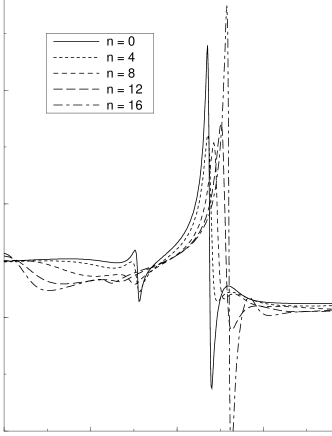
FIG. 3.: Real part of the self-energy, Re$[\Sigma({\bf k},\omega)]$ vs $\omega$ for various momenta along the diagonal of the Brillouin zone. Same parameters as in Fig.  1.

FIG. 4.: $-{\rm Im}[G_{2}({\bf q},\omega)]$ vs $\omega$ for different momenta along the diagonal of the Brillouin zone, ${\bf q}=(m,m)\pi/16$. Same parameters as in Fig.  1.

FIG. 5.: Quasiparticle dispersion for the two poles in the normal state at $T/t=0.2$ taken along the diagonal in the Brillouin zone for $U/t=4$, $\rho=0.1$.

FIG. 6.: Amplitudes of the two poles in the normal state at $T/t=0.2$ taken along the diagonal in the Brillouin zone for $U/t=4$, $\rho=0.1$.

FIG. 7.: Quasiparticle dispersion for the four poles in the superconducting state at $T/t=0.05$ taken along the diagonal in the Brillouin zone for $U/t=4$, $\rho=0.1$. For comparison, $T$-matrix results are included as symbols.

FIG. 8.: Amplitudes for the four poles in the superconducting state at $T/t=0.05$ taken along the diagonal in the Brillouin zone for $U/t=4$, $\rho=0.1$. For comparison, $T$-matrix results are included as symbols.

REFERENCES

• [1] Ding, H., Yokoja, T., Campuzano, J.C., Takahashi, T., Randeria, M., Norman, M.R., Mochiku, T., Kadowaki, K., Giapintzakis, J.: Nature 382, 51 (1996).
• [2] Loeser, A.G., Shen, Z.X., Dessau, D.S., Marshall, D.S., Park, C.H., Fournier, P., Kapitulnik, A.: Science 273, 325 (1996).
• [3] Micnas, R., Pedersen, M.H., Schafroth, S., Schneider, T., Rodríguez-Núñez, J.J., Beck, H.: Phys.  Rev.  B 52, 16223 (1995)
• [4] Kadanoff, L.P., Baym, G.: Quantum Statistical Mechanics. Advanced Book Classics. New York: Addison-Wesley 1989; Baym, G., Kadanoff, L.P.: Phys.  Rev. 124, 287 (1961); Baym, G.: Phys.  Rev.  127, 1391 (1962)
• [5] Micnas, R., Ranninger, J., and Robaszkiewicz, S.: Rev.  Mod.  Phys. 62, 113 (1990)
• [6] Rodríguez-Núñez, J.J., Schafroth, S., Beck, H., Schneider, T., Pedersen, M.H., Micnas, R.: Physica B 206–207, 654 (1995)
• [7] Rodríguez-Núñez, J.J., Schafroth, S., Micnas, R., Schneider, T., Beck, H., Pedersen, M.H.: J.  Low Temp.  Phys. 99, 315 (1995)
• [8] Schafroth, S., Rodríguez-Núñez, J.J.: Z. Phys. B, in press.
• [9] Nolting, W.: Z. Physik 225, 25 (1972); Nolting, W.: Grundkurs: Theoretische Physik. 7 Viel-Teilchen-Theorie. Ulmen: Zimmermann–Neufang 1992
• [10] Schneider, T., Pedersen, M.H., Rodríguez-Núñez, J.J.: Z.  Phys. B 100, 263 (1996)
• [11] Bickers, N.E., White, S.R.: Phys.  Rev.  B 43, 8044 (1991)
• [12] Haussmann, R.; Z.  Phys.  B 91, 291 (1993)
• [13] Mattuck, R.D.: A Guide to Feynman Diagrams in the Many-Body Problem. New York: Dover 1992; Eqs.  (10.18) and (15.58)
• [14] Frésard, R., Glaser, B., Wölfle, P.: J.  Phys.: Condens.  Matter 4, 8565 (1992)
• [15] Martín–Rodero, A., Flores, F.: Phys.  Rev.  B 45, 13008 (1992)
Refer to caption