Real Space Renormalization of the Chalker-Coddington Model

Abstract

We study a number of hierarchical network models related to the Chalker-Coddington model of quantum percolation. Our aim is to describe the physics of the quantum Hall transition. The hierarchical network models are constructed by combining series and parallel composition of quantum resistors. The localization-delocalization transition occurring in these models is treated by real space renormalization techniques. Essentially, the localization-delocalization transition is due to a competition between two one-dimensional localization mechanisms.

]

I Introduction

Despite the explosion of interest in and seemingly inexhaustible richness of the quantum Hall effect (QHE), surprisingly little progress has been made on what is arguably the central phenomenon associated with all incompressible quantum Hall liquids – the quantum Hall transition itself. By now the basic phenomenology is rather well-known: noninteracting electrons confined to a plane, when subjected to a fixed uniform magnetic field and a random scalar potential, exhibit quantum critical behavior at a sequence of energy eigenvalues, where the correlation length behaves as $\xi(E)\propto|E-E^{\vphantom{\dagger}}_{\rm c}|^{-\nu}$ with $\nu\approx{\textstyle{7\over 3}}$ [1, 2]. Early theories of localization in the presence of a magnetic field held that no extended states exist in two dimensions, a result derived from the corresponding “unitary class” nonlinear sigma model description of the long-wavelength physics. Experiments, however, unambiguously demonstrated the existence of extended states in the quantum Hall system. The work of Levine, Libby, and Pruisken [3] showed how a novel topological term present in the sigma model could produce the necessary critical behavior, although technical difficulties rendered the improved sigma model ineffective in providing a quantitative description of the transition (e.g. critical exponents, scaling functions, etc.) Nonetheless, the language of critical phenomena provided a very useful framework within which one could interpret experiments [4, 5]. Consider, for instance, the behavior of the Hall conductivity $\sigma_{xy}$ as a function of the variables $B$ (magnetic field), $L$ (linear system dimension), and $\Theta$ (temperature). Within the scaling regime, one can write

$$\sigma_{xy}(B,L,\Theta)={e^{2}\over h}f(|B-B^{*}|\,L^{1/\nu},|B-B^{*}|\,\Theta^{-1/z\nu})$$ (1)

where $B^{*}$ is a critical magnetic field, $z$ is the dynamic critical exponent, and $f(x,y)$ is a universal scaling function. From this expression, one finds the maximum slope $(\partial\sigma_{xy}/\partial B)^{\vphantom{\dagger}}_{\rm max}$ is proportional to $\Theta^{-1/z\nu}$; the power law divergence with decreasing $\Theta$ is in agreement with experiments, which independently show $z=1$ [6]. Numerical calculations [7] confirm the result $\nu=2.35\pm 0.02$, in tantalizing agreement with a compelling but alas nonrigorous argument that $\nu$ should be ${\textstyle{7\over 3}}$ [8].

One of the most significant developments in modeling the QHE transition has been the advent of the Chalker-Coddington network model of quantum percolation [9]. The relevance of classical percolation to the quantum Hall problem was emphasized by Trugman [10]. Classical electrons in a strong magnetic field ${\bf B}=B{\hat{\bf z}}$ obey the guiding center drift equations of motion

$${d{\bf r}\over dt}=-{c\over eB}\,{\hat{\bf z}}\times\nabla V({\bf r})$$ (2)

where $V({\bf r})$ is the external potential. A vivid picture emerges in which the Fermi ‘sea’ is analogous to a real sea covering a rough surface in energy space whose height is described by the function $V({\bf r})$. The corresponding quantum eigenstates are localized along equipotentials, accruing an Aharonov-Bohm phase ${\textstyle{e\over\hbar c}}\int{\bf A}\cdot d{\bf r}$ which for a complete orbit is proportional to the magnetic flux encircled (single valuedness then leads to Bohr-Sommerfeld quantization rules). Electrons at the Fermi level either circulate clockwise (as viewed from ‘above’) around isolated lakes, when $E^{\vphantom{\dagger}}_{\rm F}<\langle V\rangle$, or counterclockwise around isolated islands, when $E^{\vphantom{\dagger}}_{\rm F}>\langle V\rangle$. Such states clearly are localized. Only when $E^{\vphantom{\dagger}}_{\rm F}=E^{\vphantom{\dagger}}_{\rm c}\equiv\langle V\rangle$ are states at the Fermi level extended. As $E\to E^{\vphantom{\dagger}}_{\rm c}$, the equipotentials become more and more rarefied, and their circumference increases in size as $|E-E^{\vphantom{\dagger}}_{\rm c}|^{-4/3}$, an exact result. However, the quantum eigenfunctions are not infinitely narrow. Rather, they have a width on the order of the magnetic length $\ell=\sqrt{\hbar c/eB}$, and thus quantum tunneling will occur in the vicinity of saddle points of $V({\bf r})$ [8, 11]. It is precisely this physics which is captured by the network model. Thus, rather than directly computing the eigenfunctions of

$${\cal H}={1\over 2m}({\bf P}+{e\over c}{\bf A})^{2}+V(\bf r)\ ,$$ (3)

many of which are tightly localized on peaks and valleys and hence irrelevant to the physics of the QHE transition, the network model “cuts to the chase” and simulates a network of saddle points (see fig. 1), each described by an $S$-matrix

$$\pmatrix{{\cal O}\cr{\cal O}^{\prime}\cr}=S\pmatrix{{\cal I}\cr{\cal I}^{\prime}\cr}\ ,\ S=\pmatrix{t&r^{\prime}\cr r&t^{\prime}\cr}$$ (4)

relating incoming to outgoing flux amplitudes [9]. In the frame of an incoming electron, scattering is either to the left, with probability $T=|t|^{2}=|t^{\prime}|^{2}$, or to the right, with probability $R=|r|^{2}=|r^{\prime}|^{2}=(1-T)$ – there is neither ‘forward’ nor ‘backward’ scattering.

When $T<{\textstyle{1\over 2}}$, scattering is predominantly to the right, corresponding to the aforementioned clockwise motion around isolated lakes. Hence there is a correspondence between the energy eigenvalue $E$ for the Hamiltonian of eq. (3) and the transmission probability $T$; the quantum critical point should lie at $T={\textstyle{1\over 2}}$. Randomness enters the network model principally through phases acquired by the flux amplitudes in the course of their propagation along each link. These phases reflect the Aharonov-Bohm phases accrued due to motion along equipotential segments of irregularly varying length. The phases on the links are therefore modeled as random variables uniformly distributed between $0$ and $2\pi$. Several numerical investigations [7, 9, 12, 13] have convincingly demonstrated the applicability of the network model to the quantum Hall transition.

FIG. 1.: The Chalker-Coddington network model of quantum percolation.

In this paper, we adopt a real space renormalization group (RG) scheme which will allow us to compute exponents and scaling functions associated with the quantum Hall transition. Inasmuch as real space renormalization is fraught with uncontrolled approximations, our results will be of dubious quantitative value. However, we find that a simple and appealing qualitative picture emerges from this approach, and we feel its pedagogical value alone merits publication. We also wish to draw the reader’s attention to the recent work of Galstyan and Raikh [14], who independently developed a real space RG approach to the network model. Their results, of which we became aware when this paper was in its final stages of preparation, are largely complementary to those presented here.

II The Distribution $P_{L}(T)$

We commented above how a Chalker-Coddington network composed of identical scatterers should exhibit a quantum critical point when $T=R={\textstyle{1\over 2}}$. Consider now a network in which the individual scattering probabilities $T$ (as well as the phases on the links) are random variables, chosen from a distribution $P(T)$. We shall be interested in how the distribution $P^{\vphantom{\dagger}}_{L}(T)$ behaves with increasing cell size $L$ in the limit $L\to\infty$. To define the transmission coefficient $T$ of a finite network, we cut out a $\sqrt{2}L\times\sqrt{2}L$ section from an infinite network (the lattice spacing is $a\equiv 1$), and retain only the central $V(L)=L^{2}+(L-1)^{2}$ scattering vertices. Fig. 2 shows the $L=3$ case. Note that there are $M=2L-1$ scattering nodes across each of the main diagonals. Integrating over the random phases on the links, one obtains the distribution $P^{\vphantom{\dagger}}_{L}(T)$ for transmission to the left through the supercell.

FIG. 2.: Transmission and reflection through a $3\sqrt{2}\times 3\sqrt{2}$ network ($L=3$). The 13 vertices are denoted by black dots.

In the limit $L\to\infty$, we expect two stable distributions, given by $P^{\vphantom{\dagger}}_{\infty}(T)=\delta(T)$ and $P^{\vphantom{\dagger}}_{\infty}(T)=\delta(1-T)$. These correspond to bulk localized phases with $T=0$ and $T=1$, respectively. The quantum critical point will be characterized by an unstable distribution $P^{\vphantom{\dagger}}_{\infty}(T)=P^{*}(T)$. The terms “stable” and “unstable” refer to renormalization group flows [15]: we shall develop an approximation scheme by which the distribution $P^{\vphantom{\dagger}}_{bL}(T)$ for a larger system may be determined in terms of $P^{\vphantom{\dagger}}_{L}(T)$. This functional relation may be represented in terms of a set of parameters $\{X_{i}(L)\}$ which characterize the distribution $P^{\vphantom{\dagger}}_{L}(T)$ (e.g. the coefficients in a Legendre or Chebyshev polynomial expansion of $P^{\vphantom{\dagger}}_{L}(T)$ in the variable $x=2T-1$):

$$X_{i}(bL)=F_{i}(\{X_{j}(L)\};b)\ .$$ (5)

When $X_{i}^{*}=F_{i}(\{X_{j}^{*}\};b)$ the distribution is at a fixed point. The eigenvalues $\{\lambda_{k}\}$ of the matrix $R_{ij}=(\partial F_{i}/\partial X_{j})\big{|}_{{\vec{X}}^{*}}$ determine the relevance of the corresponding eigenvectors (scaling variables) and hence the stability of the fixed point – positive eigenvalues correspond to relevant variables and an unstable fixed point, negative eigenvalues to irrelevant variables. The positive eigenvalues define a set of critical exponents, $y^{-1}_{k}=\ln b/\ln\lambda_{k}$; the localization length exponent $\nu=\ln b/\ln\lambda_{\rm max}$ is the largest of these. One can also define the beta function

$$\beta_{i}(\{X_{j}\})={dX_{i}\over d\ln L}={\partial F_{i}\over\partial b}\Big{|}_{b=1}\ ;$$ (6)

the beta function vanishes at all fixed points.

From these considerations it becomes clear that one possible way to compute the critical exponent $\nu$ would be to determine the RG flow of $P^{\vphantom{\dagger}}_{L}(T)$. An exact procedure would require the calculation of this distribution for finite networks of arbitrary size. Computational limitations would render such attempts futile beyond even modest values of $L$. Instead, we shall resort to two uncontrolled and closely-related approximations: (i) Migdal-Kadanoff (MK) bond shifting, and (ii) replacing the square lattice with an unphysical, hierarchically constructed lattice. These approaches will allow us to perform the renormalization recursively, using only simple numerical computations.

III Series and Parallel Propagation

The group ${\rm U}(2)$ of unitary $2\times 2$ matrices may be parameterized by four angles $(\alpha,\beta,\gamma,\theta)$:

$$S=e^{i\alpha}\pmatrix{e^{i\beta}&0\cr 0&e^{-i\beta}\cr}\pmatrix{\cos\theta&\sin\theta\cr-\sin\theta&\cos\theta\cr}\pmatrix{e^{i\gamma}&0\cr 0&e^{-i\gamma}\cr}.$$

The phase angles $\alpha$, $\beta$, and $\gamma$ can be absorbed by the random link phases, and hence without loss of generality one may restrict attention to $S$-matrices of the form

$$S=\pmatrix{\cos\theta&\sin\theta\cr-\sin\theta&\cos\theta\cr}\ .$$ (7)

FIG. 3.: (a) The $S$-matrix relates incoming to outgoing flux amplitudes (see eq. (4)). This information may alternately be expressed as a transfer matrix $M$ relating left and right flux amplitudes (b), or $N$ relating top and bottom flux amplitudes (c).

This $S$-matrix may be recast in the form of a “left-to-right” transfer matrix $M$, which relates flux amplitudes ${\cal O}$ and ${\cal I}^{\prime}$ to ${\cal I}$ and ${\cal O}^{\prime}$:

$$\pmatrix{{\cal O}\cr{\cal I}^{\prime}} = M\pmatrix{{\cal I}\cr{\cal O}^{\prime}}$$

$$M = \pmatrix{\sec\theta&\tan\theta\cr\tan\theta&\sec\theta\cr}\ .$$

The transmission coefficient $T$ relating the incident flux $|{\cal I}|^{2}$ to the outgoing flux $|{\cal O}|^{2}$ is $T=\cos^{2}\theta$, and the reflection coefficient is $R=1-T=\sin^{2}\theta$.

Consider now the “series” transmission through two consecutive scatterers. Multiplying transfer matrices, and taking into account the random phases accrued in between scatterers, one obtains a composite transfer matrix

$${\widetilde{M}}=\pmatrix{\sec\theta_{2}&\tan\theta_{2}\cr\tan\theta_{2}&\sec\theta_{2}\cr}\pmatrix{e^{i\alpha}&0\cr 0&e^{i\beta}\cr}\pmatrix{\sec\theta_{1}&\tan\theta_{1}\cr\tan\theta_{1}&\sec\theta_{1}\cr}$$

and from $\sec^{2}\theta^{\prime}=|{\widetilde{M}}_{1,1}|^{2}=1/T^{\prime}$, a transmission coefficient

$${1\over T^{\prime}}={1\over T_{1}}\cdot{1\over T_{2}}\cdot\left[1+2\sqrt{R_{1}R_{2}}\cos\phi+R_{1}R_{2}\right]\ ,$$ (8)

where $\phi=\alpha-\beta$ is random. Precisely this calculation was done by Anderson et al. [16] in their study of one-dimensional localization (see also refs. [17, 18]. Averaging $\ln T$ over the angle $\phi$, one obtains

$$\langle\ln T^{\prime}\rangle=b\,\langle\ln T\rangle$$ (9)

for $b$ scatterers in series. Thus, $\ln T$ is driven to increasingly negative values – this is the essence of one-dimensional localization.

FIG. 4.: The horizontal ‘bricklayer’s representation’ of the network model. Quantum mechanical particles propagate in the directions of the arrows; scattering processes are represented by the dotted lines. The corresponding vertical representation is rotated by $90^{\circ}$.

Equivalently, though, one may view the propagation as “top-to-bottom”, and define a transfer matrix $N$ relating ${\cal O}^{\prime}$ and ${\cal I}^{\prime}$ to ${\cal I}$ and ${\cal O}$:

$$\pmatrix{{\cal O}^{\prime}\cr{\cal I}^{\prime}} = N\pmatrix{{\cal I}\cr{\cal O}}$$

$$N = \pmatrix{-\csc\theta&{\rm ctn}\,\theta\cr-{\rm ctn}\,\theta&\csc\theta\cr}\ .$$

In this case, the roles of $T$ and $R$ are reversed: $T=\sin^{2}\theta$, $R=\cos^{2}\theta$, and two scatterers in parallel give

$${1\over R^{\prime}}={1\over R_{1}}\cdot{1\over R_{2}}\cdot\left[1+2\sqrt{T_{1}T_{2}}\cos\phi+T_{1}T_{2}\right]\ ,$$ (10)

with

$$\langle\ln R^{\prime}\rangle=b\,\langle\ln R\rangle$$

for $b$ parallel scatters. In this case the reflection amplitude is driven to zero. Now in the network model, both series as well as parallel propagation occur, and in our viewpoint it is a competition between these two one-dimensional localization mechanisms which leads to a critical point corresponding to the quantum Hall transition. It is, however, impossible to neatly separate the two modes of propagation, and we shall have to resort to approximation schemes, such as the Migdal-Kadanoff approach, or to a modification of the original model, such as hierarchical network constructions, in order to make progress.

FIG. 5.: The first step in the $b=2$ Migdal-Kadanoff renormalization of the network model. Compare with fig. 4. Dashed lines indicate bonds which have been shifted to the left. Dotted lines indicate unshifted bonds.

IV Migdal-Kadanoff Approach

In order to apply the Migdal-Kadanoff bond shifting scheme to the network model, we begin by graphically representing the elementary scattering process as a kind of interaction vertex, as depicted in fig. 3. Thus, the entire network may be represented by an infinite sequence of parallel lines on which currents flow in alternating directions, and backscattering processes which divert flux from one line to one of its neighbors (see fig. 4). We call this the ‘bricklayer’s representation’ of the network model, for obvious reasons, and further describe the propagation as being either ‘horizontal’ or ‘vertical’. To effect a rescaling by a factor $b$, we start with the (horizontal) bricklayer’s representation, shown in fig. 4. In every other row, we then shift $b-1$ out of every $b$ interaction lines so as to form a new network in which each renormalized vertex represents $b$ bare vertices in series. This is depicted for $b=2$ in fig. 5. We then rescale horizontal distances by $b$. Were we to proceed in this manner, we would obtain the one-dimensional localization of ref. [16]. Instead, we view the network again in the bricklayer’s representation, this time with vertical propagation, and perform a second bond-shifting operation. This replaces each scattering vertex with an effective composite vertex, shown in fig. 6. The new network resembles that of fig. 7.

To see how this leads to critical behavior, consider the behavior of the typical transmission coefficient, $\exp\langle\ln T\rangle$, under such a transformation. From eq. (9), we obtain

$$T^{\prime}=1-(1-T^{b})^{b}\equiv f(T;b)\ ,$$ (11)

where we implicitly are working with typical values. For the case $b=2$, we have

$$f(T;b=2)=2T^{2}-T^{4}\ ,$$

which has two stable fixed points at $T^{*}=0$ and $T^{*}=1$, and one unstable fixed point at $T^{*}={\textstyle{1\over 2}}(\sqrt{5}-1)\approx 0.618$. Linearizing about the unstable fixed point, we obtain an eigenvalue $(\partial f(T;b=2)/\partial T)^{\vphantom{\dagger}}_{T^{*}}=6-2\sqrt{5}$, corresponding to a localization length exponent of $\nu=\ln b/\ln\lambda\approx 1.635$. Note that $T^{*}\neq{\textstyle{1\over 2}}$, a consequence of the order in which the bond shifting was performed: the composite vertex corresponds to series followed by parallel propagation (note the composite vertex of fig. 6 are not symmetric under $90^{\circ}$ rotations). We could equally well have chosen parallel followed by series propagation, which would switch the roles of $T$ and $R$. We note that the RG equation (11) and its counterpart with $T$ replaced by $1-T$ coincide with two RG equations obtained in a Migdal-Kadanoff approach to classical bond percolation [19]. There, the bond occupation probability $p$ plays the role of $T$, and the MK bond shifting which leads to the composition of quantum resistors in the network model corresponds to multiplication of bond occupation probabilities.

FIG. 6.: The composite vertex in the $b=2$ Migdal-Kadanoff renormalization, which corresponds to series followed by parallel propagation.

If we set $b=1+\zeta$, where $\zeta\to 0$, we obtain equations for an ‘infinitesimal’ Migdal-Kadanoff renormalization:

$$T^{\prime}=T+\zeta\left[T\ln T-(1-T)\ln(1-T)\right]+{\cal O}(\zeta^{2})\ .$$ (12)

The infinitesimal MK transformation has a fixed point at $T^{*}={\textstyle{1\over 2}}$, and an eigenvalue $\lambda=2(1-\ln 2)\zeta$, corresponding to a critical exponent of $\nu=1/2(1-\ln 2)\approx 1.629$. The MK beta function is then

$$\beta(T) = {d\over d\zeta}\bigg{|}_{\zeta=0}f(T;1+\zeta)$$ (13)

$$= T\ln T-(1-T)\ln(1-T)\ ;$$ (14)

this is shown in fig. 8.

FIG. 7.: After shifting in both the horizontal and vertical directions, each vertex in the network represents a composite of $b^{2}$ vertices. The case $b=2$ is shown here.

In statistical mechanics applications, such as the Ising model, one can define a new Hamiltonian ${\cal H}^{\prime}$ in which bonds have been shifted according to the MK prescription. When computing the partition function, one can in principle perform thermodynamic perturbation theory in $({\cal H}^{\prime}-{\cal H})$ in order to systematically improve upon the MK procedure. We know of no such systematic improvement for our scheme, nor do we have any sort of reliable estimate for the errors involved in the calculation of $\nu$.

FIG. 8.: The $\beta$-function resulting from the infinitesimal Migdal-Kadanoff renormalization. $T=0$ and $T=1$ are attractive fixed points; the critical point lies at $T={\textstyle{1\over 2}}$. Arrowheads point in the direction of RG flow.

V Hierarchical Lattices

A related approach to the problem involves the construction of hierarchical lattices. Consider, for example, the scattering unit of fig. 9, which contains $V=5$ vertices in an area $M^{2}$; in units of the distance between vertices, we have $M=3$. Now replace each of the vertices with a replica of the original cell, forming the structure shown in fig. 10. Repeating the process $n$ times generates a hierarchical structure with $V^{n}$ vertices contained in a square of side length $M^{n}$. The Hausdorff dimension of this hierarchical lattice is $D^{\vphantom{\dagger}}_{\rm H}=\ln V/\ln M\approx 1.465$. From $V(M)={\textstyle{1\over 2}}(M^{2}+1)$, one has $\lim_{M\to\infty}D^{\vphantom{\dagger}}_{\rm H}(M)=2$. The renormalization flow of the transmission coefficient and the multifractal spectrum $f(\alpha)$ was calculated in ref. [20] for the cases $M=3$, $M=5$, and $M=9$; the results for $\nu$ and $f(\alpha)$ rapidly converge to the network model results even for such modest sizes. The RG equations for the case $M=3$ are identical to those obtained in ref. [14], where a different interpretation is adopted.

FIG. 9.: An $M=3$, $V=5$ elementary cell on which a hierarchical lattice is based.

FIG. 10.: The hierarchical lattice at the second level of construction, beginning with the $M=3$, $V=5$ cell of fig. 9. There are $V^{2}=25$ vertices in this $M^{2}\times M^{2}=9\times 9$ supercell.

If one replaces the central scatterer in fig. 9 with one for which $T=1$, one recovers the four site scattering unit of fig. 6. One can use this as the fundamental unit of a hierarchical construction, and the results differ from those of the previous section only in that the linear dimension is taken to be $M=2b-1$ rather than $b$. The Hausdorff dimension of the hierarchical lattice is $D^{\vphantom{\dagger}}_{\rm H}=\ln b^{2}/\ln M$ ($=\ln 4/\ln 3$ for $b=2$), whereas the lattice of fig. 7 is fully two-dimensional. The exponent $\nu$ now is changed: $\nu=\ln M/\ln\lambda=\ln 3/\ln(6-2\sqrt{5})\approx 2.592$. Generalizations to other values of $b$ are straightforward: iterating eq. (11) $n$ times, we obtain the flow equation

$$T(M^{n}\ell_{0})=f^{[n]}(T(\ell_{0});b={\textstyle{1\over 2}}M+{\textstyle{1\over 2}})\ ,$$ (15)

where $f^{[n]}$ is the iterated function satisfying

$$f^{[n+1]}(T;b)=f\left(f^{[n]}(T;b)\right)$$

and $f^{[1]}\equiv f$. Since $f(T;b)$ is monotonically increasing from $f(0;b)=0$ to $f(1;b)=1$, there are always three fixed points on the interval $T\in[0,1]$: $T=0$ and $T=1$ (both stable), and a nontrivial unstable fixed point with $0<T^{*}<1$. The critical exponent $\nu$ is

$$\nu={\ln M\over\ln f^{\prime}(T^{*};{\textstyle{1\over 2}}M+{\textstyle{1\over 2}})}$$ (16)

where $f^{\prime}(T;b)=df(T;b)/dT$.

Whereas the Hausdorff dimension $D^{\vphantom{\dagger}}_{\rm H}$ and fixed point both increase monotonically, with

$$D^{\vphantom{\dagger}}_{\rm H}(b=1)=1\quad \quad D^{\vphantom{\dagger}}_{\rm H}(b=\infty)=2$$ ,

$$T^{*}(b=1)={\textstyle{1\over 2}}\quad \quad T^{*}(b=\infty)=1\ ,$$ ,

the critical exponent $\nu$ exhibits a minimum for $b\approx 35$, where $\nu\approx 2.11$. We find that $\nu$ diverges weakly (as $\ln b/\ln\ln b$) in the $b\to\infty$ limit. These results are plotted in fig. 11.

FIG. 11.: Results of the hierarchical lattice renormalization of eq. (15) for the fixed point transmission coefficient, $T^{*}$ (solid curve), and the localization length exponent, $\nu$ (dashed curve), versus $\ln b$. The linear dimension is $M=2b-1$.

VI Renormalization Group for Distributions

In section IV, we derived RG flows for the typical transmission coefficient, defined by $T_{\rm typ}\equiv\exp\langle\ln T\rangle$. Now we will concern ourselves with the RG flow for the entire distribution $P(T)$. We will choose the simplest nontrivial unit cell, namely that of fig. 6, in which two composite scatterers, each of which is two bare scatterers in series, are placed in parallel.

Starting with a distribution function $P(T)$, we derive the intermediate distribution $P^{\vphantom{\dagger}}_{\rm int}$ after taking two scatterers in series:

$$P^{\vphantom{\dagger}}_{\rm int}(T) = \int_{0}^{1}\!\!\!dT_{1}\,P(T_{1})\int_{0}^{1}\!\!\!dT_{2}\,P(T_{2})\times$$ (18)

$$\quad\times\int_{0}^{\pi}\!\!{d\phi\over\pi}\,\delta(T-f(T_{1},T_{2},\cos\phi))$$

with

$$f(T_{1},T_{2},\mu)={T_{1}\,T_{2}\over 1+(1-T_{1})(1-T_{2})+2\mu\sqrt{(1-T_{1})(1-T_{2})}}\ .$$

We now combine two of these composite units in parallel, obtaining the renormalized transmission coefficient distribution

$${\widetilde{P}}(T) = \int_{0}^{1}\!\!\!dR_{1}\,P^{\vphantom{\dagger}}_{\rm int}(1-R_{1})\int_{0}^{1}\!\!\!dR_{2}\,P^{\vphantom{\dagger}}_{\rm int}(1-R_{2})\times$$ (20)

$$\quad\times\int_{0}^{\pi}\!\!{d\phi\over\pi}\,\delta(1-T-f(R_{1},R_{2},\cos\phi))\ .$$

This is equivalent to the following:

$$P^{\vphantom{\dagger}}_{\rm int}(T) = {1\over 2\pi T^{2}}\int_{0}^{1}\!\!\!dT_{1}\int_{0}^{1}\!\!\!dT_{2}\,(T_{1})\,P(T_{2})\,{\Theta(1-|A|)\over\sqrt{1-A^{2}}}\times$$

$$\qquad\times{T_{1}\,T_{2}\over\sqrt{(1-T_{1})(1-T_{2})}}$$

$$A = {T_{1}\,T_{2}-T(1+(1-T_{1})(1-T_{2}))\over 2T\sqrt{(1-T_{1})(1-T_{2})}}$$

followed by

$${\widetilde{P}}(T) = {1\over 2\pi(1-T)^{2}}\int_{0}^{1}\!\!\!dT_{1}\int_{0}^{1}\!\!\!dT_{2}\,P^{\vphantom{\dagger}}_{\rm int}(T_{1})\,P^{\vphantom{\dagger}}_{\rm int}(T_{2})\times$$

$$\quad\times{\Theta(1-|B|)\over\sqrt{1-B^{2}}}\,{(1-T_{1})(1-T_{2})\over\sqrt{T_{1}\,T_{2}}}$$

$$B = {(1-T_{1})(1-T_{2})-(1-T)(1+T_{1}\,T_{2})\over 2(1-T)\sqrt{T_{1}\,T_{2}}}\ .$$

Note that $B(T_{1},T_{2};T)=A(1-T_{1},1-T_{2};1-T)$.

We have numerically iterated the distribution according to these equations. Since we expect a single relevant scaling variable controlling the RG flow of $P(T)$, we parameterize the initial distribution by its average $\langle T\rangle^{\vphantom{\dagger}}_{\rm init}$ and a width $(\Delta T)^{\vphantom{\dagger}}_{\rm init}=\sqrt{\langle T^{2}-\langle T\rangle^{2}\rangle}$. By varying $\langle T\rangle^{\vphantom{\dagger}}_{\rm init}$ alone, we drive the system through its critical point. This is shown in fig. 12, where the iterated average transmission coefficient is plotted for several initial values of $\langle T\rangle$. (We used an initial distribution which was a sum of linear plus exponentially increasing terms, though the precise details are presumably unimportant. Keeping the initial width fixed and varying $\langle T\rangle^{\vphantom{\dagger}}_{\rm init}$ between $0.605$ and $0.606$, we found the critical point $\langle T\rangle^{*}$ at $\langle T\rangle^{\vphantom{\dagger}}_{\rm init}\approx 0.60536$.) The fixed point distribution itself is plotted in fig. 13.

Within the hierarchical lattice approach, each iteration rescales the linear system size by a factor $M=3$. Analyzing the iterated average transmission coefficient $\langle T\rangle$ as a function of the number $N$ of iterations allows for the computation of $\nu$ from

$$\langle T\rangle^{\vphantom{\dagger}}_{N}-\langle T\rangle^{*}\propto M^{N/\nu}\ .$$ (21)

In fig. 14 we plot $\ln|(\langle T\rangle_{N}-\langle T\rangle^{*})/\langle T\rangle^{*}|$ versus $N\ln M$; we find $\nu\approx 6.6$. Note that within the MK scheme, the rescaling factor is $b=2$, consequently $\nu\approx 4.2$.

FIG. 12.: The RG flow of the distribution $P(T)$. The average transmission coefficient $\langle T\rangle$ is plotted versus iteration for various initial conditions. The initial value of $\Delta T$ was held fixed as $\langle T\rangle^{\vphantom{\dagger}}_{\rm init}$ was varied between $0.605$ and $0.606$. The critical point was found to lie at $\langle T\rangle^{\vphantom{\dagger}}_{\rm init}\approx 0.60536$.

FIG. 13.: The fixed distribution $P^{*}(T)$ obtained by iteration of the RG flow equations. Shown are results of a numerical integration (dotted curve) and a smooth fit to the numerical data (solid curve).

FIG. 14.: To derive $\nu$ from eq. 21, we plot the logarithm of the left hand side versus $N\ln M$. The slope is then $\nu^{-1}$. Here we show results for $M=3$ discussed in sec. VI; we find $\nu\approx 6.6$, in poor agreement with the accepted value $\nu\approx{\textstyle{7\over 3}}$.

The iteration of the full distribution function $P(T)$ according to eqs. (18,20) yields an exact RG flow for $P^{\vphantom{\dagger}}_{L}(T)$ for the four site scattering unit of fig. 6. However, the iteration could be performed only numerically. We conclude this section with a brief account of an analytical method to obtain $P(T)$. In the context of one-dimensional localization eq. (8) has been used to derive a Fokker-Planck equation (cf. [21]) for the distribution function $P^{\vphantom{\dagger}}_{L}(T)$. One identifies $T_{1}\equiv T(L)$ with the transmission coefficient of a one-dimensional resistor of length $L$ placed in series with a resistor of infinitesimal length and transmission coefficient $T_{2}\equiv T(\delta L)$. In a regime of ‘local weak scattering’, one can identify the elastic mean free path $l_{\rm e}$ by $l_{\rm e}=\delta L/\langle R(\delta L)\rangle$ and derive the following Fokker-Planck equation by standard methods (cf. [18] and references therein):

$$l_{\rm e}\,{\partial P^{\vphantom{\dagger}}_{L}(T)\over\partial L}={\partial\over\partial T}\left\{(1-T)\,{\partial\over\partial T}\,\left(T^{2}P^{\vphantom{\dagger}}_{L}(T)\right)\right\}$$ (22)

This is an equation describing one-dimensional localization. It turns out that $l_{{\rm e}}$ sets the scale for the localization length, i.e. $\langle-\ln T\rangle^{\vphantom{\dagger}}_{L}=L/l_{\rm e}$.

We now try to extend this one-dimensional scheme to the network model. Our two-dimensional iteration scheme is graphically depicted in fig. 15. We begin with an $L\times L$ array and attach to it two infinitesimal rectangles of size $L\times\delta L$ and $\delta L\times(L+\delta L)$, respectively. Transport then takes place according to the usual series and parallel composition laws. The main obstacle in deriving a Fokker-Planck equation for this model is due to the fact that we do not know a priori how the transmission coefficients of the infinitesimal blocks behave. To make progress, we proceed in analogy to the one-dimensional case and assume

$$\langle R(L,\delta L)\rangle = \langle-\ln T\rangle^{\vphantom{\dagger}}_{L}\cdot(\delta\!L/L)$$ (23)

$$\langle T(\delta L,L+\delta L)\rangle = \langle-\ln(1-T)\rangle^{\vphantom{\dagger}}_{L}\cdot(\delta\!L/L)\ .$$ (24)

With this assumption the resulting Fokker-Planck equation reads

$${\partial\over\partial L}P^{\vphantom{\dagger}}_{L}(T)=-{\partial\over\partial T}{\cal J}(T;L)\ ,$$ (25)

where the ‘current’ is given by

$${\cal J}(T;L) = \langle\ln T\rangle^{\vphantom{\dagger}}_{L}\,{1-T\over 2L}\,{\partial\over\partial T}\left\{T^{2}P^{\vphantom{\dagger}}_{L}(T)\right\}]+$$ (27)

$$\quad+\,\langle\ln(1-T)\rangle^{\vphantom{\dagger}}_{L}\,{T\over 2L}\,{\partial\over\partial T}\left\{(1-T)^{2}P^{\vphantom{\dagger}}_{L}(T)\right\}.$$

Without going into details we report on the results that one can obtain from the Fokker-Planck equation (25). We find that there are three fixed point distributions: $\delta(T)$, $\delta(1-T)$, and a uniform critical distribution $P^{*}(T)\equiv 1$. To extract the critical exponent $\nu$ of the localization length we took $X^{\vphantom{\dagger}}_{L}=\langle\ln(1-T)\rangle^{\vphantom{\dagger}}_{L}-\langle\ln T\rangle^{\vphantom{\dagger}}_{L}$ as a scaling variable which has a fixed point value $X^{*}=0$. Linearizing the flow equation around the fixed point distribution gives rise to a beta function for $X^{\vphantom{\dagger}}_{L}$ which reads

$${dX^{\vphantom{\dagger}}_{L}\over d\ln L}=X^{\vphantom{\dagger}}_{L}\ .$$ (28)

Consequently, the critical exponent is $\nu=1$. Although the Fokker-Planck approach to the network model is able to describe the correct qualitative physics of the localization-delocalization transition, it suffers from an ambiguity in modeling the average transmission coefficients of the infinitesimal blocks. Adopting a different model can change the critical exponent $\nu$. In addition, the composition laws on which the Fokker-Planck approach is based do not lead to the full Chalker-Coddington network.

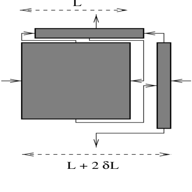
FIG. 15.: Construction of a network by adding infinitesimal networks to a square network of linear size $L$. The infinitesimal networks are characterized by a small extension $\delta L$ in one direction. The network is composed according to series and parallel composition laws.

VII Conclusion

In this paper we developed a simple approach to the quantum Hall transition. We considered a number of hierarchical network models related to the Chalker-Coddington model of quantum percolation. The basic ingredients of our networks are series and parallel compositions of quantum resistors; their hierarchical nature allows us to analyze their critical properties using simple real space renormalization techniques. In particular we studied network models that can be interpreted as resulting either from Migdal-Kadanoff bond-shifting scheme or from the construction of hierarchical lattices of Hausdorff dimension $D^{\vphantom{\dagger}}_{\rm H}<2$. The different models are labeled by an integer $b$ where $b^{2}$ is the number of resistors that form an elementary cell.

In sec. VI we calculated the flow of the distribution function $P^{\vphantom{\dagger}}_{L}(T)$ for the transmission coefficient $T$ (‘two-point-conductance’) in the case $b=2$. This was done by means of numerically iterating the renormalization group equations. We found the flow to have three fixed points, two of which correspond to localization ($T\equiv 0$, $T\equiv 1$). The third fixed distribution $P^{*}(T)$ corresponds to the quantum critical point, where delocalization occurs. The critical point distribution $P^{*}(T)$ turned out to be very broad and the flow of $P^{\vphantom{\dagger}}_{L}(T)$ in the vicinity of $P^{*}(T)$ is governed by one-parameter scaling. The critical exponent $\nu$ was also determined and found in poor agreement with accepted values.

As a further simplification we derived renormalization schemes for the typical transmission coefficient, $T_{\rm typ}\equiv\exp\langle\ln T\rangle$. Here, we simply averaged over the random link phases, neglecting variations in the individual transmission coefficients. We obtained closed RG equations for $T_{\rm typ}$ (secs. IV,V). From these equations we derived fixed point values for $T_{\rm typ}^{*}(b)$ and critical localization length exponents $\nu^{\vphantom{\dagger}}_{b}$ for arbitrary $b>1$. For small $b$ the notion of typical transmission coefficient as a substitute for a whole distribution (which is broad) is dubious and it is no surprise that $\nu^{\vphantom{\dagger}}_{b=2}$ differs from the value obtained by iterating the whole distribution function. However, the notion of typical transmission coefficient is more reliable for large $b$ where the composition of $b$ resistors in series favors the formation of log-normal type distributions. On the other hand, for large $b$ the resulting hierarchical network has little in common with the original Chalker-Coddington network. Nevertheless, the slow variation of $\nu^{\vphantom{\dagger}}_{b}$ with $b$ shows that the results for intermediate $b$ are not too far from that of the original network model.

All models that we considered exhibit a localization-delocalization transition which results from a competition between two one-dimensional quantum mechanical localization mechanisms. The models result from uncontrolled approximations to the network model, but have at least some pedagogical value. In contrast to the well-known classical percolation model for quantum Hall transitions, our models are essentially quantum mechanical. Furthermore, the concept of real space renormalization can be extended to improve quantitative results (see refs.  [14],[20]).

While this manuscript was in the final stage of preparation, we discovered the work of ref. [14] in which a similar real space renormalization group approach to the Chalker-Coddington model is developed. In that work an elementary $M=3$, $V=5$ cell (see fig. 9) replaces each scatterer in the renormalization step. (In addition, the rescaling factor in [14] is $b=2$ rather than $M=3$.) In our work the central scatterer of this cell is replaced with one for which $T=1$ (or $R=1$), resulting in the simple series-parallel composition laws discussed above.

VIII Acknowledgements

DPA and MJ would like to thank the Physics Department at Technion, where this work was started. DPA also thanks the Lady Davis Fellowship Trust and the National Science Foundation, grant NSF DMR-91-13631, for partial support. MJ also thanks the MINERVA foundation and the Sonderforschungsbereich 341 of the Deutsche Forschungsgemeinschaft for partial support. We are grateful to A. Weymer for discussions and for assistance in computing the exponent in sec. VI.

REFERENCES

- [1] Alternatively, one can fix the energy and vary the magnetic field. The integer QHE transition separates states of filling fraction which are consecutive integers. In interacting systems, the quantum Hall transition it believed to be related to that of a corresponding noninteracting system after a sequence of transformations: (Landau level raising), (particle-hole conjugation), and (flux attachment). For a discussion of these and other related ideas, see S. Kivelson, D.-H. Lee, S.-C..Zhang, Phys. Rev. B 46, 2223 (1992).
- [2] The Quantum Hall Effect, R. E. Prange and S. M. Girvin, eds. (Springer-Verlag, Berlin, 1994); M. Janssen, O. Viehweger, U. Fastenrath, and J. Hajdu, Introduction to the Theory of the Integer Quantum Hall Effect (VCH, Weinheim, 1994).
- [3] H. Levine, S. Libby, and A. M. M. Pruisken, Phys. Rev. Lett. 51, 1915 (1983).
- [4] A. M. M. Pruisken, Phys. Rev. Lett. 61, 1297 (1988).
- [5] S. L. Sondhi, S. M. Girvin, J. P. Carini, and D. Shahar, preprint cond-mat/9609279.
- [6] L. W. Engel, D. Shahar, Ç. Kurdak, and D. C. Tsui, Phys. Rev. Lett. 71, 2638 (1993).
- [7] B. Huckestein, Rev. Mod. Phys. 67, 357 (1995).
- [8] G. V. Mil’nikov and I. M. Sokolov, JETP Lett. 48, 536 (1988).
- [9] J. T. Chalker and P. D. Coddington, J. Phys. C 21, 2665 (1988).
- [10] S. A. Trugman, Phys. Rev. B 27, 7539 (1983); M. Tsukada, J. Phys. Soc. Japan 41, 1466 (1976).
- [11] H. A. Fertig and B. I. Halperin, Phys. Rev. B 36, 7969 (1987); J. K. Jain and S.. Kivelson, Phys. Rev. B 37, 4111 (1988); H. A. Fertig, Phys. Rev. B 38, 996 (1988).
- [12] D.-H. Lee, Z.-Q. Wang, and S. Kivelson, Phys. Rev. Lett. 70, 4130 (1993).
- [13] R. Klesse and M. Metzler, Europhys. Lett. 32, 229 (1995).
- [14] A. G. Galstyan and M. E. Raikh, preprint cond-mat/9701010.
- [15] J. L. Cardy, Scaling and Renormalization in Statistical Physics (Cambridge Univ. Press, Cambridge, 1996).
- [16] P. W. Anderson, D. J. Thouless, E. Abrahams, and D.S. Fisher, Phys. Rev. B 22, 3519 (1980).
- [17] P. Mello, J. Math. Phys. 27, 2876 (1986); Phys. Rev. B 35, 1082 (1987).
- [18] B. Shapiro, Phil. Mag. B 56, 1031 (1987).
- [19] S. Kirkpatrick, Phys. Rev. B 15, 1533 (1977). These equations also appear in the context of site percolation in B. Shapiro, J. Phys. C 13, 3387 (1980).
- [20] A. Weymer and M. Janssen, unpublished (1997).
- [21] H. Risken, The Fokker-Planck Equation, (Springer-Verlag, Berlin, 1989).