Repton model of gel electrophoresis in the long chain limit

Abstract

Reptation governs motion of long polymers through a confining environment. Slack enters at the ends and diffuses along the polymer as stored length. The rate at which stored length diffuses limits the speed at which the chain can drift. This paper relates the rate of stored length diffusion to the conformation of the tube within which the polymer is confined. In the scaling limit of long polymer chains and weak applied electric fields, holding the product of polymer length times field finite, the tube length and stored length density take on their zero-field values. The drift velocity then depends only on the the polymer’s end-to-end separation in the direction of the field.

1 Introduction

Gel electrophoresis separates charged polymers, such as sections of DNA, according to their length. Applied electric fields exert a uniform force per unit length parallel to the field. The gel contains pores and fibers which tend to entrap the long polymers within tubes [1] (see figure 1), impeding their drift. Significant motion of the polymer occurs by the transport of stored length through the tube, a process known as reptation [2]. As a result of entanglement of the polymer in the gel, the polymer develops a complicated dependence of drift velocity on electric field ${\cal E}$ and total polymer length ${\cal L}=l_{p}N$. We denote the polymer persistence length (typically of order 150-300 base pairs for DNA) as $l_{p}$, and call $N$ the “chain length” of the polymer.

In the limit of weak field, the velocity is proportional to the electric force through the Nernst-Einstein relation

$$v_{d}={{D}\over{k_{B}T}}(qN{\cal E}).$$ (1)

Here $(qN{\cal E})$ is the electric force on the polymer, with $q$ the charge within a persistence length. The diffusion constant $D$ depends on the chain length according to the prediction of de Gennes [2]

$$D\sim N^{-2}.$$ (2)

Comparing equations (1) and (2), the weak field drift velocity varies inversely with the chain length. Short chains travel more quickly than long chains, and chains may be sorted according to length based on their travel time across the gel, or their travel distance within a given time.

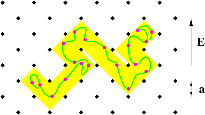
Figure 1: Polymer (solid curve) entangled in gel (squares) confined to tube (shaded area). Dots spaced at intervals of $l_{p}$ are called reptons.

Loss of length resolution, a serious impediment to electrophoresis as a separation tool, occurs for any polymer above a certain length. For DNA typical limits [3] are of order 50 Kbp, with chain length $N$ of order 150-300. Increasing these limits requires reducing the electric field, thus increasing the run time, or using more delicate gels. Pulsed-field [3] and other techniques push the threshold length out yet further, reaching DNA lengths of order $10^{7}$ bp, with chain length $N$ of order $10^{5}$. From a mathematical point of view, loss of length resolution implies a breakdown of the Nernst-Einstein relation between drift velocity and zero-field diffusion constant. Understanding this problem requires further investigation of the functional form of the drift velocity $v_{d}(N,{\cal E})$.

Length and field dependence of the drift velocity have been well studied analytically for biased reptation models [4]. These models assume constant tube length and conformation, independent of the applied electric field and independent of time. They conclude that diffusion of stored length depends only on the polymer tube length and end-to-end distance. Their dynamics is random polymer reptation biased by the applied electric field. Rubenstein [5] introduced what is now called the “repton model” (see figures 1 and 2), a lattice model that dynamically generates its own tube. Later Duke [6] generalized the repton model to include the electric field. Semenov, Duke and Viovy [7] introduced fluctuations directly into the biased reptation model.

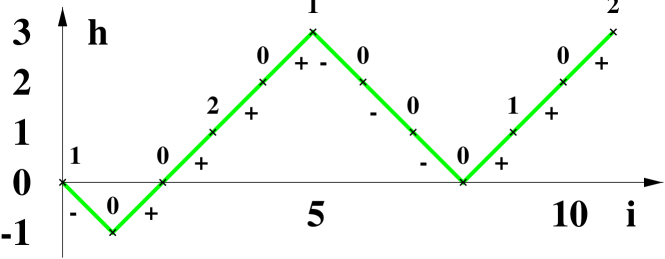
Figure 2: Repton model in the $({\bf n};{\bf s})$ representation. The numbers along the chain denote $n_{i}$, while the $\pm$ signs define $s_{i}$ . This configuration represents the polymer displayed in figure 1. The horizontal axis labels gel pores in sequence along the tube. The horizontal axis represents the height $h_{i}$ with respect to the first pore $i=0$. In this figure L=11, S=+3, $N_{0}$=7, N=19

The Repton model was studied intensively by B. Widom and co-workers [8, 9, 10], and by van Leeuwen and co-workers [11, 12, 13], among others. It is convenient to introduce fundamental length and frequency parameters $a$ and $\omega$, and to define a reduced electric field $E=|q{\cal}E|a/k_{B}T$. Numerical simulations by Barkema, Marko and Widom [9] suggest a simple scaling behavior for the drift velocity, with

$${{N^{2}}\over{a\omega}}v_{d}(N,E)\rightarrow J(NE)$$ (3)

in the scaling limit

$$E\rightarrow 0,\hskip 28.45274ptN\rightarrow\infty,\hskip 28.45274ptu\equiv NE\hskip 14.22636pt{\rm finite}$$ (4)

They suggest an approximate functional form for the scaling function

$$J(u)\approx u\sqrt{\left({{1}\over{3}}\right)^{2}+\left({{2u}\over{5}}\right)^{2}}.$$ (5)

This scaling function exhibits loss of length resolution because at fixed fields the drift velocity varies as $E|E|$, independent of N for long chain lengths. Barkema, Caron and Marko [14] discovered similar scaling relations for real DNA fragments and electrophoresis gels.

The repton model decomposes the polymer chain into $N$ units called reptons, each incorporating one persistence length of the chain. When neighboring reptons on the chain lie within the same gel pore a unit of stored length separates them. Otherwise the reptons must occupy neighboring gel pores, because the bond between reptons prevents further excursions. Label the occupied gel pores with index $i=0,2,...,L$. The bond from one pore $i-1$ to the neighboring pore $i$ we denote $s_{i}=\pm 1$, where $i=1,2,...L$. The direction of pore labeling $i$ is chosen as follows: the “head” of the polymer is the end that is furthest advanced in the direction of applied force. The other end is the “tail”. Labeling begins at the tail and runs to the head. As the polymer drifts, head and tail may occasionally interchange. The set of all bonds ${\bf s}$ defines the shape of the polymer’s tube.

Reptons may move along the tube when attached to at least one unit stored length. Stored length is recorded in the variable $n_{i}$ for the units of stored length in gel pore $i$. The set of stored length occupancy data for all gel pores is denoted ${\bf n}$. The total amount of stored length, summed over gel pores, is $N_{0}$=N-1-L. When a repton moves it carries a unit of stored length from the pore which it left into the new pore. The potential energy of the polymer changes by $Es_{i}$ when a unit of stored length moves from pore $i-1$ to $i$. The center of mass of the polymer advances by $s_{i}a/N$. Allowed moves occur with frequency $\omega B^{s_{i}}$ where the Boltzmann factor $B=e^{E/2}$. The electric field favors either left- or right-wards motion depending on the sign of $s_{i}$.

The tube constantly changes shape while stored length migrates across the polymer. However, the changes in tube conformation for short times occur in a small length around the ends of the polymer. The time for stored length to traverse the tube is small compared to the time required for significant change in polymer conformation. This is clearly the case for zero field diffusion, because de Gennes [2] showed that the time required for tube renewal $\tau_{R}$ grows as $N^{3}$, while the diffusion of a unit of stored length takes the usual $\tau_{S}\sim N^{2}$ time to travel a distance N. Thus the tube renewal time exceeds the time for stored length relaxation by a factor N.

The factor of N, by which $\tau_{R}$ exceeds $\tau_{S}$ persists for finite fields. Each unit of stored length that traverses the tube advances the polymer by one gel pore. Generation of a new tube therefore requires $L$ units of stored length to diffuse across the polymer. Tube length $L$ is proportional to chain length N.

Examine the distance from each end of the polymer over which diffusion of stored length is sensitive to fluctuations in tube conformation. Denote this length scale $l_{c}$, and note that the time scale for stored length diffusion across this length is $l_{c}^{2}$. The time needed for renewal of this length of tube varies as $l_{c}^{3}$ because $l_{c}$ units of tube length must diffuse a distance of order $l_{c}$. The length at which these time scales are comparable defines $l_{c}$, of order $1$. Further from the ends of the tube, the tube is effectively stationary while stored length diffuses. More information about the coupling of stored length diffusion to chain conformation near the chain ends may be found in reference [12].

We use the idea of fixed tube conformation on the time scale of stored length diffusion to simplify the analytic solution of the repton model with free boundaries. By appropriately adjusting the dynamics at the free ends, we achieve closed form expressions for the drift velocity as a function of tube conformation. These expressions reproduce the drift velocity of the original repton model in the limit of long polymer chains.

2 Stored length diffusion

The joint probability distribution $P({\bf n};{\bf s})$ defines the probability for tube conformation ${\bf s}$ and stored length distribution ${\bf n}$ within the tube. This function obeys the steady-state master equation

$$\sum_{{\bf n}^{\prime}{\bf s}^{\prime}}W({\bf n}^{\prime}{\bf s}^{\prime}\rightarrow{\bf n}{\bf s})P({\bf n}^{\prime};{\bf s}^{\prime})=\sum_{{\bf n}^{\prime}{\bf s}^{\prime}}W({\bf n}{\bf s}\rightarrow{\bf n}^{\prime}{\bf s}^{\prime})P({\bf n};{\bf s})$$ (6)

The left hand side is the rate of transitions into the state $({\bf n};{\bf s})$, while the right hand side is the rate of transitions out of that state. Approximate solution of this master equation follows the observation that stored length diffuses quickly compared to changes in tube conformation, except within distances of order 1 of the tube ends. Fluctuations at the tube endpoints have negligible impact on the stored length probability distribution away from the tube ends.

We replace the original free boundary repton model described by the master equation (6) with a simpler model in which the tube conformation ${\bf s}$ is held fixed. The simpler master equation

$$\sum_{i=0}^{L}\theta(n_{i})\left[\right.B^{-s_{i+1}}P(\cdot\cdot\cdot,n_{i}-1,n_{i+1}+1,\cdot\cdot\cdot;{\bf s})+$$

$$B^{s_{i}}P(\cdot\cdot\cdot,n_{i-1}+1,n_{i}-1,\cdot\cdot\cdot;{\bf s})\left.\right]$$ (7)

$$=\sum_{i=0}^{L}\theta(n_{i})\left[B^{s_{i+1}}+B^{-s_{i}}\right]P({\bf n};{\bf s}).$$

may be solved exactly. The first term on the left describes the flux of stored length from gel pore $i+1$ into $i$. The second term describes flux from $i-1$ to $i$. The right-hand side of equation (2) describes flux out of site $i$. The summations include as-yet undefined functions of stored length occupation and bond orientation just beyond each end-point of the tube. We define the probability function $P({\bf n};{\bf s})$ to be independent of the variables $n_{-1}$ and $n_{L+1}$, and we introduce fictitious bonds $s_{0}=s_{L+1}=0$. This is equivalent to placing the tube in contact with a reservoir of freely available stored length at each end.

Our simpler model is identical to the periodic-boundary repton model studied by Van Leeuwen and Kooiman [11] with the exception of the boundary condition. The drift velocity of sufficiently long chains is not influenced by our alteration of the endpoint dynamics because it is diffusion of stored length along the interior of the tube that limits the drift velocity. The solution to equation (2) yields the stored length distribution within a tube of fixed conformation ${\bf s}$, but no information on the probability distribution for tube conformations. Equation (2) has a well known solution [15]

$$P({\bf n};{\bf s})=\prod_{i=0}^{L}p_{i}^{n_{i}}.$$ (8)

Formally we extend this solution beyond the tube endpoints by defining

$$p_{-1}\equiv p_{L+1}\equiv 1$$ (9)

in order that $P({\bf n};{\bf s})$ not depend on $n_{-1}$ and $n_{L+1}$. The form of solution (8) with free ends is identical to the solution with periodic boundary conditions [11, 15], because the master equation is a local difference equation.

The analysis that follows is largely adapted from the studies of the periodic boundary repton problem, and the free boundary problem in weak fields, by Van Leeuwen and co-workers [11, 12, 13]. Our approach is exact in the large $N$ limit for the free end repton model in arbitrary electric field. The factors $p_{i}$ obey the single-particle master equation

$$B^{-s_{i+1}}p_{i+1}+B^{s_{i}}p_{i-1}=\left[B^{s_{i+1}}+B^{-s_{i}}\right]p_{i}.$$ (10)

The single-particle master equation (10) is second order, so the solution depends on two independent constants of integration.

One constant of integration is the flux of stored length through each bond

$$c({\bf s})\equiv p_{i-1}B^{s_{i}}-p_{i}B^{-s_{i}}.$$ (11)

Although the left hand side of equation (11) formally depends on $i$, the value of $c$ is independent of $i$. The boundary condition $p_{-1}=1$, governing the availability of stored length at chain ends, sets the other constant of integration. The full solution is

$$p_{i}=p_{-1}B^{2h_{i}}-c\sum_{k=0}^{i}B^{2(h_{i}-h_{k})+s_{k}}$$ (12)

where we define

$$h_{i}=\sum_{j=1}^{i}s_{j}$$ (13)

the “height” of the tube in the direction parallel to the field, as indicated in figure 2.

The form of solution (12) is interesting. The first term is the “barometric” distribution of stored length, the expected equilibrium distribution in the absence of flux. An equivalent distribution occurs in the original repton model, when one repton is held fixed so the polymer cannot drift [16]. The second term corrects for the steady flow of particles. Since the boundary conditions (9) apply at both ends of the chain, the stored length flux $c({\bf s})$ is determined. Setting $p_{L+1}=1$ in equation (12), we solve for

$$c({\bf s})={{B^{2S}-1}\over{\sum_{k=0}^{L+1}}B^{2(S-h_{k})+s_{k}}}.$$ (14)

In this expression, we define

$$S=\sum_{i=1}^{L}s_{i}.$$ (15)

as the end-to-end separation parallel to the field $E$. This quantity equals the height at the end of the tube.

Given the probability distribution $P({\bf n};{\bf s})$ we calculate the tube-dependent velocity

$$v({\bf s})=\sum_{{\bf n}}P({\bf n};{\bf s})v({\bf n};{\bf s})/\sum_{{\bf n}}P({\bf n};{\bf s}).$$ (16)

Here the the imbalance of forward and backward transition rates for stored length within the tube governs the velocity associated with a particular allocation of stored length,

$$v({\bf n};{\bf s})={{a\omega}\over{N}}\sum_{i=0}^{L}\theta(n_{i})(s_{i+1}B^{s_{i+1}}-s_{i}B^{-s_{i}}).$$ (17)

We include the natural velocity scale for the problem $a\omega/N$, with $a/N$ the center of mass displacement parallel to the field for each repton jump, and $\omega$ the jump attempt frequency. Once we know the velocity for arbitrary tubes, we approximate the full drift velocity $v_{d}$ as an average of $v({\bf s})$ over tube conformations ${\bf s}$.

It is convenient to interchange the summations over ${\bf n}$ in equation (16) with the sum over $i$ in equation (17). Then

$$v({\bf s})={{a\omega}\over{N}}\sum_{i=0}^{L}\bar{\theta_{i}}(s_{i+1}B^{s_{i+1}}-s_{i}B^{s_{i}})$$ (18)

where $\bar{\theta_{i}}$ is the average of $\theta(n_{i})$ over the allocation of stored length

$$\bar{\theta_{i}}=\sum_{{\bf n}}P({\bf n};{\bf s})\theta(n_{i})/\sum_{{\bf n}}P({\bf n};{\bf s}).$$ (19)

Using the exact solution for $P({\bf n};{\bf s})$ equation (8),

$$\bar{\theta_{i}}=\sum_{{\bf n}}\theta(n_{i})\prod_{j=0}^{L}p_{j}^{n_{j}}/\sum_{{\bf n}}\prod_{j=0}^{L}p_{j}^{n_{j}}.$$ (20)

The theta function picks out terms that contain at least one unit of stored length in gel pore $i$.

Removing the obvious factor of $p_{i}$ from the numerator of equation (20), the remaining factors are partition functions for the distribution of stored length among gel pores,

$$Q(N_{s})=\sum_{{\bf n}}\prod_{j=0}^{L}p_{j}^{n_{j}}\hskip 14.22636pt{\rm with}\hskip 14.22636pt\sum_{j=0}^{L}n_{j}=N_{s}.$$ (21)

The sums in equation (20) allocate $N_{s}=N_{0}$ units of stored length in the denominator but only $N_{s}=N_{0}-1$ units in the numerator. The ratio

$$\bar{z}({\bf s})\equiv Q(N_{0}-1)/Q(N_{0})$$ (22)

is the fugacity for stored length. Hence

$$\bar{\theta_{i}}=p_{i}\bar{z}({\bf s})$$ (23)

is the explicit solution of equation (19).

Substitute expression (23) for $\bar{\theta_{i}}$ into equation (18) for $v({\bf s})$. Utilizing the fictitious bonds $s_{0}=s_{L+1}=0$ to shift the summation index on the first term of equation (18), yields

$$v({\bf s})={{a\omega\bar{z}({\bf s})}\over{N}}\sum_{i=0}^{L}(p_{i-1}B^{s_{i}}-p_{i}B^{-s_{i}})s_{i}.$$ (24)

The quantity in parentheses above is the single particle flux defined in equation (11). In particular, it is independent of $i$, and may be brought outside the sum. Finally, we obtain our principal result

$$v({\bf s})={{a\omega Sc({\bf s})\bar{z}({\bf s})}\over{N}}$$ (25)

This equation is fully general, holding for any field and any tube conformation. The relationship of $v({\bf s})$ to the repton model drift velocity $v_{d}$ depends on the limit of long chains. We conjecture the average over all tubes ${\bf s}$ of $v({\bf s})$ equals the drift velocity $v_{d}$ with corrections of order $1/N$ relative to $v_{d}$ caused by our fixed-tube boundary conditions.

3 Scaling limit

In the scaling limit (4) the electric field vanishes as $1/N$, leading to significant simplifications. For weak fields, we simplify equation (14) for the single-particle flux by expanding in powers of E

$$c({\bf s})={{SE}\over{L+2}}+{\cal O}(E^{2}S^{2}/L)$$ (26)

Interestingly, this value of $c$ exactly counterbalances the barometric term in equation (27), ensuring that the first order term in $p_{i}$ grows only as EN^1/2 even if the end-to-end distance $S$ grows proportionally to N. It inhibits the tendency of stored length to accumulate at favorable positions on the chain. The simple form for the flux $c$ arises because $s_{i}E$ is the force along any link between gel pores, so $SE$ is the net force along the tube, and $SE/L$ the net force per link.

Simplify equation (12) for $p_{i}$ by expanding

$$p_{i}=1+Eh_{i}-(i+1)c+{\cal O}(E^{2}h_{i}^{2}).$$ (27)

Then substitute $p_{i}=1+{\cal O}(E)$ into the partition functions $Q$ defined in equation (21) to obtain the fugacity

$$\bar{z}({\bf s})={{N_{0}}\over{N_{0}+L}}+{\cal O}(ES^{2}/L)$$ (28)

with $N_{0}+L=N-1$.

Inserting equation (26) for flux $c({\bf s})$ and equation (28) for fugacity $\bar{z}({\bf s})$ into equation (25) for velocity, we obtain the expression

$$v({\bf s})={{a\omega N_{0}S^{2}E}\over{N^{2}L}}$$ (29)

with corrections expected to fall off as $1/N$ in the scaling limit. Van Leeuwen and coworkers derived similar equations for the repton model in weak fields. Similar expressions are also known for biased reptation models [4, 7]. We conjecture that equation (29) is exact for the repton model with free boundary conditions in the scaling limit for all values of the scaling variable $u=NE$. We make a further conjecture, that equation (29) gives the drift velocity $v_{d}$ with $N_{0}$, $L$ and $S$ set to their average values.

One immediate result of expression (29) is the zero-field diffusion constant. Since $S^{2}=L=2N/3$ at zero field, the weak-field drift velocity is simply $a\omega(NE)/3N^{2}$, in agreement with the accepted diffusion constant $D=1/3N^{2}$. Hence our conjectures hold at least at $u=0$.

4 Numerical study and discussion

To test our conjecture that equation (29) holds throughout the scaling limit (4) we calculate averages of L, $S^{2}$ and $v({\bf s})/v_{d}$ for various values of the scaling variable $u=NE$, and then extrapolate to large chain lengths N. We test the conjecture for moderate and large $u=1$ and $10$. For short chain lengths, N=3-7 we perform exact calculations based on the matrix approach described in reference [8]. Because the matrix dimensionality grows as $3^{N}$ it is impractical to extend these calculations to large N. Instead, we perform numerical simulation of drift using the multi-spin simulation program of Gerard Barkema [9]. During these simulations we monitor $S^{2}$ and $L$ in addition to the drift velocity.

Figure 3: Moderate field $NE=1$ data. $L/(N-1)$, $S^{2}/(N-1)$ and $v({\bf s})/v_{d}$ are shown, respectively, in parts a, b and c.

Figure 4: Strong field $NE=10$ data. $L/N$, $S^{2}/N$, and $v({\bf s})/v_{d}$ are shown, respectively, in parts a, b and c.

Figures 3 and 4 display our results for $\overline{L}/(N-1)$ and $\overline{S^{2}}/(N-1)$, and the ratio $v({\bf s})/v_{d}$ calculated by inserting average values of $L$ and $S^{2}$ into equation (29) for the velocity in weak fields. We divide $L$ and $S^{2}$ by N-1, because the finite size correction then vanishes in the limit $u=NE~{}\rightarrow 0$. Data for small N=3-7 are exact matrix calculations, while data for large $N$ are simulated.

It appears that $\overline{L}/(N-1)\rightarrow 2/3$ for any value of the scaling variable $u$. Dashed lines in figures 3a and 4a indicate the value $2/3$. The finite size correction falls off proportionally to $u/N$. Our analysis of the scaling limit in section (3) explains these results. Assuming that $\overline{S^{2}}$ equals $N$ times a function of $u$, equation (28) predicts the fugacity takes its zero-field value with finite-size corrections of order $E=u/N$. The stored length density $N_{0}/L$, which depends on the fugacity, inherits the zero-field value and $u/N$ finite-size correction and in turn passes them on to $\overline{L}/(N-1)$.

In contrast, the asymptotic value of $\overline{S^{2}}$ depends on the scaling variable $u$. Variation of the end-to-end separation causes the entire functional dependence of drift velocity on $E$ and $N$, because $\overline{N_{0}}$ and $\overline{L}$ are constants in the scaling limit. References [7] and [9] predict a cigar-shape polymer conformation for large values of $u$, with elongation parallel to the field of order $N|E|^{1/2}$. Assuming that the head and tail of the polymer lie near the top and bottom of this cigar shape, we identify the elongation with our variable $S$. From equation (29) it follows that the large $u$ drift velocity varies as $E|E|$ independent of $N$, consistent with the large $u$ form of $J(u)$.

Examining parts $c$ of figures 3 and 4, we see that in the large $N$ limit, the velocity predicted by the weak field limit (29) converges to the actual simulated velocity. The large $N$ behavior is consistent with the ratio of equation (29) to simulated velocity approaches $1$ as $1/N^{\sigma}$ with the power $\sigma$ falling between $1/2$ and $1$. This holds for small, moderate and large values of the scaling variable, because finite-size and -field corrections vanish in the scaling limit.

In conclusion, we present a general formula (25) for the drift velocity of any tube conformation in any electric field. The simpler result (29) applies throughout the scaling limit of long chains at fixed $u=NE$. Our approach works because diffusion of stored length decouples from fluctuations of chain conformation except over a negligible length near the ends of the chain. The velocity is governed entirely by the end-to-end separation of the tube S. Tube fluctuations [7] are important only because they permit dependence of $\overline{S^{2}}$ on $u$.

References

- [1] S.F. Edwards, Molecular Fluids, eds. R. Balian and G. Weill (Gordon and Breach, 1976)
- [2] P.G. de Gennes, Scaling Concepts in Polymer Physics (Cornell University Press, 1979)
- [3] D.C. Schwartz and C.R. Cantor, Cell 37 (1984) 67-75
- [4] L.S. Lerman and H.L. Frisch, Biopolymers 21 (1982) 995-997; O.J. Lumpkin and B.H. Zimm, Biopolymers 21 (1982) 2315-2316; G.W. Slater and J. Noolandi, Phys. Rev. Lett. 55 (1985) 572
- [5] M. Rubinstein, Phys. Rev. Lett. 59 (1987) 1946
- [6] T.A.J. Duke, Phys. Rev. Lett. 62 (1989) 2877
- [7] A.N. Semenov, T.A.J. Duke and J.-L. Viovy, Phys. Rev. E51 (1995) 1520 introduces tube fluctuations directly into the biased reptation model.
- [8] B. Widom, J.L. Viovy and A.D. Desfontaines, J. Phys. (Paris) I 1 (1991) 1759
- [9] G.T. Barkema, J.F. Marko and B. Widom, Phys. Rev. E 49 (1994) 5303
- [10] A.B. Kolomeisky and B. Widom, Physica A229 (1996) 53-60
- [11] J.M.J. van Leeuwen and A. Kooiman, Physica A 184 (1992) 79
- [12] J.D. Balkenende, J.A. Leegwater and J.M.J. van Leeuwen, 25 Years of Non-Equilibrium Statistical Mechanics, Proceedings of the 13th Sitges Conference, eds. J.J. Brey, et al. (Springer-Verlag, 1995) p. 211
- [13] J.A. Leegwater and J.M.J. van Leeuwen, Phys. Rev. E 52 (1995) 2753; J.A. Leegwater, Phys. Rev. E 52 (1995) 2801
- [14] G.T. Barkema, C. Caron and J.F. Marko, Biopolymers 38 (1996) 665
- [15] B. Derrida, J. Stat. Phys. 31 (1983) 433
- [16] B. Widom (unpublished)