Competition in a Fitness Landscape

1 Introduction

In this paper we address the problem of formation of species in simple ecosystems, possibly mirroring some aspects of bacterial and viral evolution. Our model can be considered as an extension of Eigen’s model [1, 2]. With respect to the latter, we introduce the interactions among individuals.

The correspondence of this kind of models with real biological systems is rather schematic: the (haploid) organisms are only represented by their genetic information (the genotype), and we do not consider sexuality nor age structure or polymorphism. Moreover, a spatial mean field approximation is applied, so that the relevant dynamical quantity is the distribution of genotypes. This distribution evolves under the combined effects of selection and mutations. Selection is represented by the concept of fitness landscape [3, 4], a function of the genotype that represents the average fraction of survivors per unit of time, and includes the effects of reproductive efficiency, survival and foraging strategies, predation and parassitism, etc. In other words, the fitness function is the evolutive landscape seen by a given individual. Only point mutations are considered, and these are assumed to be generated by independent Poisson processes. The presence of mutations allows the definition of the distance between two genotypes, given by the minimum number of mutations required to connect them. Assuming only point mutations, the genotypic space is a hypercube, each direction being spanned by the possible values of each symbol in the sequence. In the Boolean case, which is the one considered here, each point mutation connects two vertices along the axis corresponding to the locus where the mutation has taken place.

In the original work, Eigen and Schuster [2] showed that a landscape with a single maximum of the fitness allows for a phase transition from a bell-shaped distribution of the population centered at the location of the maximum of the fitness function (the master sequence) to a flatter distribution. This error transition is triggered by the mutation rate.

It has been shown [5, 6] that Eigen’s model is equivalent to an equilibrium statistical mechanical model of interacting spins, the latter being the elements of the genome. In this way several evolutionary concepts can be mapped to a statistical mechanics language. In particular, for a static fitness landscape, the evolution becomes the process of optimization of an “energy” function (the logarithm of the fitness), balanced by the entropy. The genealogy of a particular genome can be represented as a two-dimensional spin system. We refer to the two directions as the time and the genotypic one, respectively. The coupling in the time direction is ferromagnetic and is given by the mutations. The coupling in the genotypic direction is given by the fitness function and is in general long range. While this mapping is suggestive and allows a precise characterization of vaguely defined terms, from the point of view of numerical and analytical treatments of the equations, the original differential equation approach is more effective.

Borrowing the language of statistical mechanics, the single sharp maximum case (the one studied originally by Eigen and Schuster [2]) can be defined as a degenerate genotypic space, since all individuals but the master sequence have the same fitness, and we consider it as a particular case of the more general class of genotypic spaces in which the fitness depends only on the genotypic distance from the master sequence.

The degenerate landscape can be represented as a linear one by introducing the appropriate multiplicity factor. Using this approach, one implicitly assumes that all degenerate strains are evenly populated, i.e., that there exist high transition rates among these strains. This assumption has been exploited in the study of the phase diagram of the single sharp maximum case [7].

Finally, assuming a hierarchy for the relevance of mutations, one can have a pure linear genotypic space. For instance, let us consider Boolean sequences of length $L$ and assume that $000\dots$ is the master sequence. Deleterious mutations $0\rightarrow 1$ are assumed to be non-lethal only if they accumulate at the ends of the sequence, as (for $L=3$)

$$111\leftrightarrow 110\leftrightarrow 100\leftrightarrow 000\leftrightarrow 001\leftrightarrow 011\leftrightarrow 111,$$ (1)

where the arrows denote the mutations. One can introduce a genotypic index $-3\leq x\leq 3$ and rewrite eq. (1) as

$$-3\leftrightarrow-2\leftrightarrow-1\leftrightarrow 0\leftrightarrow 1\leftrightarrow 2\leftrightarrow 3\equiv-3,$$

i.e., we have a linear genotypic space with periodic boundary conditions.

An hypothetical example of such a hierarchical space is that of a series of genes that code for enzymes involved in a metabolic pathway. A mutation in the first enzyme of the sequence is more likely lethal, while a mutation that lowers the affinity of the last enzyme with its substrate could be easily retained even if the fitness of the individual is lowered. This mutation reduce also the specificity of the last enzyme with its substrate (which is the product of the previous metabolic step), allowing a mutation in the previous enzyme and so on.

Almost all the works dealt with abstract landscapes (mainly RNA world). The difficulty in applying these concepts to real biological systems concerns the definition of the fitness function, that relates the genotype to the phenotype. In particular, the difficulty resides in predicting the stability or the efficiency of a protein given its sequence of amino acids. One can circumvent this difficulty taking into consideration only the subclass of all possible mutations that do not change the protein structure. One example of an explicit definition of the fitness function is given by the variation of the reproductive rate of bacteria due to synonymous mutations and tRNA usage [8, 9]. This study can be considered an example of a degenerate smooth maximum fitness landscape. Another explicit biological application concerns the evolution of RNA viruses on HeLa cultures [10]. In this case the fitness landscape was assumed to be linear (without multiplicity).

While in general the fitness landscape depends on the presence of others individuals and changes with time, it is much simpler to study the problem for a given (static) landscape, that can be thought as an approximation for diluted, rapidly evolving organisms or self-catalytic molecules (RNA world), while all other species remain constant. In these static landscapes, all strains are coupled by the normalization of the probability distribution, and for small values of the mutation rate (a situation fulfilled in the real case) and smooth landscapes, the fittest quasi-species always eliminates all others [6]. The global coupling given by the normalization of probability corresponds to the case of finite population size or the alternative phases of exponential growth followed by starvation and death. For of a rugged static landscape (for instance generated by an Hopfield Hamiltonian [5, 6]), the distribution of species can reflect the distribution of the peaks of fitness. In these cases the interesting question concerns the error transition.

In this work we address the problem of species formation in presence of competition. The idea of our approach is the following: we look for a stable probability distribution formed by separated quasi-species, and for each of them we compute the effective fitness landscape due to the competition with individuals of the same and all other species. Then, the parameters of the distribution (position and weight of quasi-species) are obtained in a self-consistent way. In this way we are able to compute analytically the threshold for species formation transition in a linear landscape.

We shall deal with coupled differential and finite difference equations, that can be thought as a mean field approximation of a true microscopic model. The effect of the finiteness of population, however, should imply a cutoff on the tail of the distribution, due to the discreteness of the individuals, and thus the dependence of evolution on the initial condition (for an application of the cutoff effect, see Ref. [10]). We do not consider here these effects.

The sketch of this paper is the following: first of all, we formalize the model in section 2, then we work out the distribution of a quasi-species near a maximum of the effective fitness landscape in section 3, and finally we apply the self-consistency condition in section 4, comparing the analytical approximation with the numerical resolution. Conclusions and perspectives are drawn in the last section.

2 The model

We describe in detail the approximations that lead to our model. An individual is identified by its genome, represented by an integer index $x$ (no polymorphism nor age structure). We study the case of a linear genotypic space (hierarchical relevance of mutations).

We shall not consider here age structure nor the effects of polymorphism in the phenotype. For the sake of simplicity, we shall deal only with haploid organisms. Moreover, we do not consider the spatial structure (spatial mean field). The experimental setup of reference is that of an bacterial population that grows in a stirred liquid medium, with constant supply of food and removal of solution, so that the average size of the population is constant. Another possible experiment concerns RNA viruses [10].

We consider the distribution $p(x,t)$, that gives the probability of observing the strain $x$ at time $t$ within the population. We shall denote the whole distribution as $\boldsymbol{p}(t)$. At each time step we have

$$\sum_{x}p(x,t)=1.$$ (2)

Organisms undergo selection, reproduction and mutation. The reproduction and death rates are represented by a fitness function $A\bigr{(}x,\boldsymbol{p}(t)\bigl{)}$, that represents the average fraction of individual of a given strain $x$ surviving after a time step in absence of mutation for a given probability distribution $\boldsymbol{p}(t)$.

As usual, we consider only point mutations, and we factorize the probability of multiple mutations (i.e., they are considered independent events). The rate of mutation per time step of a single element of the genome is $\mu$; each point mutation connects the strain $x$ to $x+1$ or $x-1$.

Since we want to model existing populations, we deal with small mutation rates. In this limit, only one point mutation can occur at most during a time step. This is the main difference with previous works, in which the main goal was to study a mutation-induced phase transition (error threshold).

With these assumptions, the generic evolution equation (master equation) for the probability distribution is

$$\alpha(t)p(x,t+1)=\left(1+\mu\frac{\delta^{2}}{\delta x^{2}}\right)A\bigl{(}x,\boldsymbol{p}(t)\bigl{)}p(x,t);$$ (3)

where the discrete second derivative $\delta^{2}/\delta x^{2}$ is defined as

$$\frac{\delta f(x)}{\delta x^{2}}=f(x+1)+f(x-1)-2f(x),$$

and $\alpha(t)$ maintains the normalization of $\boldsymbol{p}(t)$. In the following we shall mix freely the continuous and discrete formulations of the problem.

The numerical resolution of eq. (3) shows that a stable asymptotic distribution exists for almost all initial conditions. In the asymptotic limit $t\rightarrow\infty$, $\boldsymbol{p}(t+1)=\boldsymbol{p}(t)\equiv\boldsymbol{p}(x)$. Summing over $x$ in eq. (3) and using the normalization condition, eq. (2), we have:

$$\alpha=\sum_{x}A(x,\boldsymbol{p})p(x)=\overline{A}.$$ (4)

The normalization factor $\alpha$ thus corresponds to the average fitness. The quantities $A$ and $\alpha$ are defined up to an arbitrary constant.

In general the fitness $A$ depends on $x$ and on the probability distribution $\boldsymbol{p}$. The dependence on $x$ includes the structural stability of proteins, the efficiency of enzymes, etc. This corresponds to the fitness of the individual $x$ if grown in isolation. On the other hand, the effective fitness seen by an individual depends also on the composition of the environment, i.e., on $\boldsymbol{p}$. This $\boldsymbol{p}$-dependence can be further split into two parts: the competition with other clones of the same strain, (intra-strain competition) and that with different strains (inter-strains competition), disregarding more complex patterns as the group structure (colonies). The intra-strain term has the effect of broadening the curve of a quasi-species and of lowering its fitness, while the inter-strains part can induce the formation of distinct quasi-species.

Since $A$ is strictly positive, it can be written as

$$A(x,\boldsymbol{p})=\exp\bigl{(}H(x,\boldsymbol{p})\bigr{)}.$$

If $A$ is sufficiently smooth (including the dependence on $\boldsymbol{p}$), one can rewrite eq. (3) in the asymptotic limit, using a continuous approximation for $x$ as

$$\alpha p=Ap+\mu\frac{\partial^{2}}{\partial x^{2}}(Ap),$$ (5)

Where we have neglected to indicate the genotype index $x$ and the explicit dependence on $\boldsymbol{p}$. Eq. (5) has the form of a nonlinear diffusion-reaction equation. Since we want to investigate the phenomenon of species formation, we look for an asymptotic distribution $\boldsymbol{p}$ formed by a superposition of several non-overlapping bell-shaped curves, where the term non-overlapping means almost uncoupled by mutations. Let us number these curves using the index $i$, and denote each of them as $p_{i}(x)$, with $p(x)=\sum_{i}p_{i}(x)$. Each $p_{i}(x)$ is centered around $\overline{x}_{i}$ and its weight is $\int p_{i}(x)dx=\gamma_{i}$, with $\sum_{i}\gamma_{i}=1$. We further assume that each $p_{i}(x)$ obeys the same asymptotic condition, eq. (5) (this is a sufficient but not necessary condition). Defining

$$\overline{A}_{i}=\frac{1}{\gamma_{i}}\int A(x)p_{i}(x)dx=\alpha,$$ (6)

we see that in a stable ecosystem all quasi-species have the same average fitness.

3 Evolution near a maximum

We need the expression of $\boldsymbol{p}$ if a given static fitness $A(x)$ has a smooth, isolated maximum for $x=0$ (smooth maximum approximation). Let us assume that

$$A(x)\simeq A_{0}(1-ax^{2}),$$ (7)

where $A_{0}=A(0)$. Substituting $q=Ap$ in eq. (5) we have (neglecting to indicate the genotype index $x$, and using primes to denote differentiation with respect to it):

$$\frac{\alpha}{A}q=q+\mu q^{\prime\prime}.$$

Looking for $q=\exp(w)$,

$$\frac{\alpha}{A}=1+\mu({w^{\prime}}^{2}+w^{\prime\prime}),$$

and approximating $A^{-1}=A_{0}^{-1}\left(1+ax^{2}\right)$, we have

$$\frac{\alpha}{A_{0}}(1+ax^{2})=1+\mu({w^{\prime}}^{2}+w^{\prime\prime}).$$ (8)

A possible solution is

$$w(x)=-\frac{x^{2}}{2\sigma^{2}}.$$

Substituting into eq. (8) we finally get

$$\frac{\alpha}{A_{0}}=\frac{2+a\mu-\sqrt{4a\mu+a^{2}\mu^{2}}}{2}.$$ (9)

Since $\alpha=\overline{A}$, $\alpha/A_{0}$ is less than one we have chosen the minus sign. In the limit $a\mu\rightarrow 0$ (small mutation rate and smooth maximum), we have

$$\frac{\alpha}{A_{0}}\simeq 1-\sqrt{a\mu}$$

and

$$\sigma^{2}\simeq\sqrt{\frac{\mu}{a}}.$$ (10)

The asymptotic solution is

$$p(x)=\gamma\frac{1+ax^{2}}{\sqrt{2\pi}\sigma(1+a\sigma^{2})}\exp\left(-\frac{x^{2}}{2\sigma^{2}}\right),$$

so that $\int p(x)dx=\gamma$. The solution is a bell-shaped curve, its width $\sigma$ being determined by the combined effects of the curvature $a$ of maximum and the mutation rate $\mu$.. In the next section, we shall apply these results to a quasi-species $i$. In this case one should substitute $p\rightarrow p_{i}$, $\gamma\rightarrow\gamma_{i}$ and $x\rightarrow x-\overline{x}_{i}$.

For completeness, we study also the case of a sharp maximum, for which $A(x)$ varies considerably with $x$. In this case the growth rate of less fit strains has a large contribution from the mutations of fittest strains, while the reverse flow is negligible, thus

$$p(x-1)A(x-1)\gg p(x)A(x)\gg p(x+1)A(x+1)$$

neglecting last term, and substituting $q(x)=A(x)p(x)$ in eq. (3) we get:

$$\frac{\alpha}{A_{0}}=1-2\mu x=0$$ for (11)

$$q(x)=\frac{\mu}{\left(\alpha A(x)-1+2\mu\right)}q(x-1) x>0$$ for (12)

Near $x=0$, combining eq. (11), eq. (12)and eq. (7)), we have

$$q(x)=\frac{\mu}{(1-2\mu)ax^{2}}q(x-1).$$

In this approximation the solution is

$$q(x)=\left(\frac{\mu}{1-2\mu a}\right)^{x}\frac{1}{(x!)^{2}},$$

and

$$y(x)=A(x)q(x)\simeq\frac{1}{A_{0}}(1+ax^{2})\left(\frac{\mu A_{0}}{\alpha a}\right)^{x}\frac{1}{x!^{2}}.$$

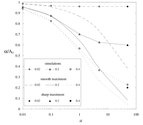
Figure 1: Average fitness $\alpha/A_{0}$ versus the coefficient $a$, of the fitness function, eq. (7), for some values of the mutation rate $\mu$. Legend: numerical resolution corresponds to the numerical solution of eq. (3), smooth maximum refers to eq. (9) and sharp maximum to eq. (11)

We have checked the validity of these approximations numerically solving eq. (3); the comparisons are shown in Figure (1). We observe that the smooth maximum approximation agrees with the numerics for for small values of $a$, when $A(x)$ varies slowly with $x$, while the sharp maximum approximation agrees with the numerical results for large values of $a$, when small variations of $x$ correspond to large variations of $A(x)$.

4 Speciation

Let us now study the stable quasi-species distribution for a simple interacting fitness landscape. The fitness $A(x,\boldsymbol{p})=\exp(H(x,\boldsymbol{p}))$ is given by

$$H(x,\boldsymbol{p})=H_{0}+H_{1}(x)+H_{2}(x,\boldsymbol{p})+\dots$$

where $H_{0}$ is an arbitrary constant, $H_{1}(x)$ is the static landscape, i.e., the fitness seen by an individual in isolation (it includes the interaction with all other slowly varying species) and $H_{2}(x,\boldsymbol{p})$ is the interaction landscape. We examine the case of a single quadratic maximum of $H_{1}$, using the explicit form:

$$H_{1}(x)=b\left(1-\frac{|x|}{r}-\frac{1}{1+\frac{|x|}{r}}\right),$$

where $r$ gives the amplitude of the quadratic maximum, and $b$ is the curvature. For $x\rightarrow\infty$, $H_{1}(x)\simeq b(1-|x|/r)$, while for $x\rightarrow 0$, $H_{1}(x)\simeq-bx^{2}/r^{2}$. We have checked numerically that other similar smooth potentials give the same results of this one.

We assume that the interactions among individuals are always negative (competition) and decrease exponentially with the distance:

$$H_{2}(x,\boldsymbol{p})=-J\int\exp\left(-\frac{\left(x-y\right)^{2}}{2R^{2}}\right)p(y)dy.$$

Figure 2: Probability distribution with five quasi-species. Numerical values are $\mu=0.01$, $H_{0}=1.0$, $b=0.2$, $J=7.0$, $R=10$ and $r=3$.

Numerically solving eq. (3) we obtain the asymptotic probability distribution showed in Figure 2. One can observe the presence of several non-overlapping quasi-species. For $R\rightarrow\infty$, substituting $p(x)=\sum_{i}p_{i}(x)$, one has

$$H_{2}(x,\boldsymbol{p})=-J\sum_{i}\gamma_{i}\exp\left(-\frac{\left(x-\overline{x}_{i}\right)^{2}}{2R^{2}}\right).$$

The location $\overline{x}_{k}$ of the maximum of the quasi-species $k$ is given by:

$$\left.\frac{dA}{dx}\right|_{\overline{x}_{k}}=0.$$

The species 0 occupies the fittest position $\overline{x}_{0}=0$. For $k\neq 0$ we have (using the large $x$ approximation for $H_{1}$):

$$-\frac{b}{r}+J\sum_{i}\gamma_{i}\frac{\overline{x}_{k}-\overline{x}_{i}}{R^{2}}\exp\left(-\frac{\left(\overline{x}_{k}-\overline{x}_{i}\right)^{2}}{2R^{2}}\right)=0.$$

We consider now the case of three species, two of which are symmetric with respect to the dominant one. We have $\overline{x}_{0}=0$, $\overline{x}_{1}=-\overline{x}_{2}=\overline{x}$. In the limit $\mu\rightarrow 0$, we can consider $\alpha=A_{0}(1-\sqrt{a\mu})=A_{0}$, and thus $\alpha=A(0)=A(\overline{x})$ (this is a strong approximation which simplifies the computation), and

$$-b+\frac{b\overline{x}}{r}+J\gamma_{1}+\frac{R^{2}b}{r\overline{x}}=J\gamma_{0}+2\frac{\gamma_{1}}{\gamma_{0}}\frac{R^{2}b}{r\overline{x}}.$$

Finally, we have the following system

$$z^{2}-G(\gamma_{0}-\gamma_{1})z+1-2\frac{\gamma_{1}}{\gamma_{0}}-z\frac{r}{R} =0,$$ (13)

$$\gamma_{0}+2\gamma_{1} =1,$$ (14)

$$G\gamma_{0}z\exp(-z^{2}/2) =1,$$ (15)

where $z=\overline{x}/R$ and $G=Jr/Rb$.

The limit of coexistence for the three species is given by $\gamma_{0}=1$ (and thus $\gamma_{1}=0$). We compute the critical value $G_{c}$ of $G$ for the coexistence of three species, in the limit $r/R\rightarrow 0$. The first order term $G_{c}^{(0)}$ is obtained computing $z$ from eq. (14)

$$z=\frac{G_{c}^{(0)}+\sqrt{{G_{c}^{(0)}}^{2}-4}}{2},$$

and inserting this value into eq. (15). Solving numerically this equation, we have $G_{c}^{(0)}\simeq 2.2160$. The first correction $G_{c}^{(1)}(r/R)$ is obtained from eq. (14), and is simply $G_{c}^{(1)}=-r/R$. So finally we have for the critical threshold of species formation $G_{c}$

$$G_{c}=2.216-\frac{r}{R}.$$ (16)

Figure 3: Behavior of $G_{c}$ versus $r/R$. The continuous line represents the analytical approximation, eq. (16), the circles are obtained from numerical resolution. The error bars represent the maximum error.

We have solved numerically eq. (3) for different values of the parameters, and we have checked that the threshold of coexistence of the three species depends only on $G$. In particular, this threshold does not depends on the mutation rate $\mu$, at least for $\mu<0.1$, which is a very high mutation rate for real organisms. The most important effect of $\mu$ is the broadening of quasi-species curves, that can eventually merge. In the range of parameters used, $G$ depends only on ratio $r/R$. Both these results are in agreement with the analytical predictions obtained above. In Figure 3 we compare the numerical and analytical results, plotting the different threshold value $G_{c}$ as function of $r/R$.

5 Discussion and conclusions

We have studied a simple model for species formation. This model can be considered an extension of Eigen’s one [1, 2], with the inclusion of competition, which if the fundamental ingredient for species formation in smooth landscapes. On the other hand, from an individual’s point of view and disregarding complex structures such as the colonial organization, the more similar the phenotype the more important the sharing of resources and thus the competition. Since we assumed a smooth dependence of phenotype on genotype, we simply modeled the competition $J(x,y)$ between the two strains $x$ and $y$ by means of a smooth function of the distance between two genotypes: $J(x,y)=-J\exp(-(x-y)^{2}/2R^{2})$. In this way the strongest competition occurs with other instances of the same strain, which is reasonable. One can interpret our interaction terms as a cluster expansion of a long-range potential, in which we retained single and two bodies contributions. From the point of view of population dynamics, our form of modeling the competition is equivalent to the Verlhust damping term (logistic equation).

In a real ecosystem, however, there could be positive contributions to the interaction term $J$. In particular, it can happen that $J(x,y)>0$ and $J(y,x)<0)$ (predation or parassitism), or $J(x,y)>0$ and $J(y,x)>0)$ (cooperation). An investigation on the origin of complexity in random ecosystems is in progress. In particular we want to study the effects of time fluctuation of fitness (say due to human interaction) on the number of coexisting species.

We have studied the effects of competition in a linear (i.e., hierarchic) genotypic space. Our results synthesize in Figure 3. The dependence of the threshold for the formation of quasi-species obtained analytically from our approximations reflects very well the numerical results. We also checked that the latter does not depend on the mutation rate $\mu$, up to $\mu=0.1$.

Acknowledgements

We wish to thank G. Guasti, G. Cocho, R. Rechtman, G. Martinez-Mekler and P.Lió for fruitful discussions. M.B. thanks the Dipartimento di Matematica Applicata “G. Sansone” for friendly hospitality. Part of this work was done during the workshop Chaos and Complexity at ISI-Villa Gualino (Torino, Italy) under CE contract ERBCHBGCT930295.

References

- [1] W. Eigen, Naturwissenshaften 58 465 (1971).
- [2] W. Eigen and P. Schuster, Naturwissenshaften 64, 541 (1977).
- [3] S. Wright, The Roles of Mutation, Inbreeding, Crossbreeding, and Selection in Evolution, Proc. 6th Int. Cong. Genetics, Ithaca, 1, 356 (1932).
- [4] L. Peliti, Fitness Landscapes and evolution http://xxx.lanl.gov/abs/cond-mat/9505003
- [5] I. Leuthäusser, J. Stat. Phys 48 343 (1987).
- [6] P. Tarazona, Phys. Rev. A 45 6038 (1992).
- [7] D. Alves and J. F. Fontanari, Phys. Rev. E 54 4048 (1996).
- [8] F. Bagnoli and P. Lió, J. Theor. Biol. 173 271 (1995).
- [9] F. Bagnoli, G. Guasti, P. Lió, Translation optimization in bacteria: statistical models, in Nonlinear Excitations in Biomolecules, M. Peyrard, Editor (Les Editions de Phisique-Springer, 1995).
- [10] L.S. Tsimring, H. Levine and D.A. Kessler, Phys. Rev. Lett. 76 4440 (1996).