Electron scattering states at solid surfaces calculated with realistic potentials

Abstract

Scattering states with low-energy-electron diffraction asymptotics are calculated for a general non-muffin tin potential, as, e.g., for a pseudopotential with a suitable barrier and image potential part. The latter applies especially to the case of low lying conduction bands. The wave function is described with a reciprocal lattice representation parallel to the surface and a discretization of the real space perpendicular to the surface. The Schrödinger equation leads to a system of linear one-dimensional equations. The asymptotic boundary value problem is confined via the quantum transmitting boundary method to a finite interval. The solutions are obtained based on a multigrid technique that yields a fast and reliable algorithm. The influence of the boundary conditions, the accuracy, and the rate of convergence with several solvers are discussed. The resulting charge densities are investigated.

Electron spectroscopies at low energies below $100$ eV are sensitive to the shape of the surface near potential. Sophisticated bandstructure calculations involve such potentials, but almost exclusively consider bound states. To obtain the same accuracy for current carrying states is still a challenge. Here we will consider final states of photoemission, which are time-reversed states of low energy electron diffraction (LEED). Typical energies of interest are $10$ eV and higher. With the advent of space-filling full-potential LEED calculations,[2] the correct surface barrier can be included, but this requires, especially at these energies, extended CPU time. Another approach relies on smooth continuous matching[3] of the solutions inside the crystal to those in the vacuum. The inclusion of the surface potential by the propagation-matrix method [4] has proven to be an ill-posed problem.[5] The reason is the formulation as an initial value problem, which does not ensure the crucial continuous dependence on the boundary values. This is guaranteed by the two-side boundary conditions.[5, 6] Modern treatments of elliptic problems often employ a discretization in direct space instead of choosing physically motivated basis functions. A recent work on LEED and low energy positron diffraction presented a three-dimensional finite-difference method.[7] For the lower energies of ultraviolet photoemission spectroscopy, the Coulomb singularities of the cores are less important. They can be avoided by using pseudopotentials, for which a mixed representation of the wave function seems to be suitable here.

In this contribution we address a direct, methodically simple, and fast solution of the Schrödinger equation with the scattering asymptotics treated as introduced by Lent and Kirkner.[8] The problem is formulated as a two-side boundary problem. The calculations refer exemplary to the GaAs (110) surface. The Schrödinger equation has to be solved for a given energy $E$ and a given direction of the electron incident on the surface with a surface parallel wave vector $\vec{k}_{\|}$. The translation symmetry parallel to the surface allows a description of the wave function $\Psi$ and the potential $V$ in the Laue representation, consisting of a Fourier decomposition in the $xy$ plane parallel to the surface with the Fourier coefficients $\varphi_{\vec{g}}$ and $V_{\vec{g}}$ depending on the coordinate $z$ of the direct space perpendicular to the surface,

$$\Psi(\vec{\rho},z) = \sum_{\vec{g}}\varphi_{\vec{g}}(z)e^{i(\vec{k}_{\|}+\vec{g})\cdot\vec{\rho}}\,,$$ (1)

$$V(\vec{r}) = \sum_{\vec{g}}V_{\vec{g}}(z)e^{i\vec{g}\cdot\vec{\rho}}+\Sigma(E,z)\;.$$ (2)

The two-dimensional vector $\vec{\rho}$ lies in the $xy$ plane, the imaginary optical potential $\Sigma$ accounts for the attenuation owing to many-particle effects and other inelastic losses. The summation is over the reciprocal lattice vectors $\vec{g}$. In the Laue representation the Schrödinger equation appears as a system of linear one-dimensional differential equations, which we discretize by a grid with step size $h_{z}$ in the $z$ direction. This leads to the linear matrix equation ${\cal A}_{h_{z}}\vec{\varphi}_{h_{z}}=0$ with the solution $\vec{\varphi}_{h_{z}}$ and the coefficients

$$({\cal A}_{h_{z}})_{i\vec{g},i^{\prime}\vec{g}^{\prime}} = \left(\frac{-\delta_{i,i^{\prime}+1}+2\delta_{i,i^{\prime}}-\delta_{i,i^{\prime}-1}}{h_{z}^{2}}\right)\delta_{\vec{g},\vec{g}^{\prime}}$$ (3)

$$+ \left[\left((\vec{g}+\vec{k_{\parallel}})^{2}+\frac{2m}{\hbar^{2}}\left(-E+\Sigma(E,i)\right)\right)\delta_{\vec{g},\vec{g}^{\prime}}\right.$$ (4)

$$+ \left.\frac{2m}{\hbar^{2}}V_{\vec{g}^{\prime}-\vec{g},i}\right]\delta_{i,i^{\prime}}\;.$$ (5)

The indices are the reciprocal lattice vectors $\vec{g}$, $\vec{g}^{\prime}$ and the grid points $i$,$i^{\prime}$. The complex matrix ${\cal A}_{h_{z}}$ is non-hermitean and indefinite. Since the potential relies on the Laue representation without any restrictions, the method allows direct application of potentials from modern band-structure computations. Nonlocal pseudopotentials can be applied in a way similar to their use in three-dimensional finite difference calculations of electronic structure.[9] For the calculation here we take as an example a potential, which was repeatedly applied to photoemission calculations of GaAs(110).[10] It is a local pseudopotential with the surface barrier taking into account relaxation, corrugation, and a smooth saturated image potential.

Equation 5 requires boundary conditions at the bulk and at the vacuum side of the grid. The simplest model of a surface potential is a single step towards the vacuum, as used in matching calculations. A first guess for boundary conditions far away from the surface inside the crystal and that outside within the vacuum are Dirichlet values taken from such preliminary calculations. In Fig. 1 the modulus of the wave functions for different grid sizes is plotted. Plots (c) and (d) show irregularities around the bulk boundary. Even with Neumann or mixed boundaries this feature cannot be suppressed. Because the damping reduces the wave functions to zero deep in the bulk, the required asymptotic behavior is fulfilled by taking a zero value at a boundary sufficiently remote from the surface. Since the damping depends on energy, the coordinate of the boundary in the bulk should be chosen as energy dependent and automatically adjusted by tracking the neighboring values of the wave function.

In the vacuum the wave functions still differ even for high grid sizes as shown in Fig. 1 (a) and (b). Therefore, we investigate this boundary more closely. In a LEED experiment a beam of electrons is scattered at the surface of the crystal. The vacuum boundary condition has to guarantee one single incoming plane wave. This can be tested by a half-sided Fourier transformation of the wave function in the vacuum, assumin that the Fourier grid is well separated from the vicinity of the surface. The solution from a matching calculation does fulfill the incoming beam asymptotics, the subsequent grid calculation with the same step potential does not. The Fourier spectrum of the grid wave function shows additional incoming ghost waves that have contributions of up to $15\%$ and thereby strongly deteriorate the physical situation. Neumann and mixed boundaries from the matching do not improve this unsatisfactory situation. Again the matching does not provide a correct boundary condition even far away from the crucial vicinity of the surface.

The correct boundary conditions in the vacuum are achieved by use of the elegant and simple quantum transmitting boundary method (QTBM).[8] The wave function in the vacuum is expanded into a set of propagating waves

$$\Psi_{vac}{(\vec{\rho},z)}=\sum_{\vec{g}}\left(\phi_{\vec{g}}^{(+)}e^{+i{\kappa}_{\vec{g}}z}+\phi_{\vec{g}}^{(-)}e^{-i{\kappa}_{\vec{g}}z}\right)e^{i(\vec{k}_{\|}+\vec{g})\cdot\vec{\rho}}\;.$$

$\phi_{\vec{g}}^{(+)}$ and $\phi_{\vec{g}}^{(-)}$ are the amplitudes of the given incoming and unknown outgoing waves, respectively. The grid wave function $\Psi_{grid}$ is that of Eq. (1). For a short description of the quantum transmitting boundary method let $LN(\,)$ be a linear function and $FT(\,)$ the two-dimensional Fourier transformation. Continuity at boundary $z_{r}$ then yields at that plane

$$\frac{\partial}{\partial z}\Psi_{vac} = LN\left(\phi_{\vec{g}}^{(+)},\phi_{\vec{g}}^{(-)}\right)=LN\left(\phi_{\vec{g}}^{(+)},FT(\Psi_{vac})\right)$$

$$= LN\left(\phi_{\vec{g}}^{(+)},FT(\Psi_{grid})\right)=LN\left(\phi_{\vec{g}}^{(+)},\varphi_{\vec{g}}(z_{r})\right)\;.$$

From the continuity of the normal derivative follows

$$\frac{\partial}{\partial z}\Psi_{grid}=LN\left(\phi_{\vec{g}}^{(+)},\varphi_{\vec{g}}(z_{r})\right)\;.$$

This mixed linear boundary value problem is the QTBM that is inserted in Eq. (5) with the derivative being discretized. The implementation of the QTBM is simple here due to the Laue representation. With the QTBM the calculated wave function fulfills the correct LEED asymptotics in the case of the step barrier as it does for any corrugated barrier too. Figure 2 shows the Fourier spectrum normal to the surface of a grid calculation with the QTBM basing either on a step potential or basing on the true barrier. The negative wave numbers correspond to incoming waves. Both solutions show the postulated LEED asymptotics of one incoming wave. The barrier potential influences strongly the solution, which is also illustrated by the plot of the wave functions in Fig. 3.

Equation (5) with the boundary conditions inserted gives a quadratic, linear, and inhomogeneous system of equations, which has a block tridiagonal coefficient matrix. As an example we consider the GaAs(110) surface with a normal incident electron beam at an energy of $E_{f}=18$ eV, which in vacuum corresponds to a kinetic energy of $E_{kin}=12.75$ eV. The lateral plane wave basis of $57$ reciprocal lattice vectors proved to be sufficient for the employed potential. With the lattice constant of $a=5.654$ Å, the boundaries are chosen to be at $\pm 15a$, enclosing $45$ layers with $90$ atoms. The large distance from the surface to the vacuum boundary ensures a sufficient decay of the image potential. The positions of the boundaries deep inside the crystal and far outside in the vacuum cause a large grid, whose step size $h_{z}$ is bounded by several conditions. First, the wave function has to be correctly represented on the grid. This bound can be estimated by use of the sampling theorem. Furthermore, a small step size is needed for a stable discretization and a safe convergence of the iterative solvers. The Laplace operator has to dominate the zero-order terms, which require $h_{z}\leq 0.06a$ here. Further bounds are given by the demands of applications. With $h_{z}=0.012a$ a typical number of $2500$ grid points and $142\,500$ equations results.

Since the coefficient matrix results from an elliptic equation, is sparse, and is additionally a band matrix, a variety of solvers are available. As for the photoemission spectra a large series of final states has to be calculated, it is very important to reduce the CPU time per final state. Several direct and iterative solvers have been tested. Some of the resulting CPU time and memory requirements are given in Table I. Time and memory increase linear with the number of grid points due to the simple structure of the coefficient matrix. The fastest direct solver was a routine in band storage mode performing an LU factorization that needs $98$ s for the test problem with a slope of $3.9\!\times\!10^{-2}s$ per grid point. It needs less than half of the time than a LEED calculation with space-filling potentials at this energy or a conventional matching at a potential step.

Iterative solvers in combination with multigrid methods are highly successful in solving differential equations.[11] They have recently been applied to the calculations of large-scale electronic structure.[12] We implemented a two- and a three-grid method. For the smoothing, the squared Jacobi iteration has been applied. With a damping factor of 0.5 the best convergence rates have been obtained. The Laue representation simplifies the implementation of the QTBM, but it causes strong codiagonals due to the potential coefficients. Therefore on the first level the equations must be treated by a direct solver, and the Jacobi iteration is only used for smoothing on the finer grids. For the step size of $0.018a$ on the coarse grid the two-grid iteration needs 20 steps to achieve the same mean defect of $\sim 10^{-14}$ as the direct solver. The three-grid methods do not improve the convergence rates. The defect after 20 iterations was for a W cycle $6\!\times\!10^{-10}$ and for a V cycle $5\!\times\!10^{-7}$. Theoretically the multigrid method needs $O(N)$ operations to solve a system of $N$ linear equations. The direct method for band matrices needs $O(Nw^{2})$ operations. Because the number of codiagonals $w$ is the constant number of reciprocal lateral lattice vectors, both methods have the same asymptotic behavior. However, if a lower accuracy of the solution is acceptable, the multigrid method becomes more favorable. If, e.g., a defect of $10^{-6}$ is sufficient, the two-grid method needs five iterations and $91$ s and gives an error in the modulus of the wave function of less than $0.2\%$. Additionally, the maximum memory used can be reduced within the multigrid method. If the system of equations is solved directly, a $(3w\!+\!1)\!\times\!N$ matrix containing the LU factorization on the fine grid is needed. In the multigrid iteration with depth $l$ the $(2w\!+\!1)\!\times\!N$ matrix on the fine grid and the $(3w\!+\!1)\!\times\!(N2^{-(l-1)})$ LU matrix on the coarse grid are stored. From the three-grid iteration onward, the required memory for the multigrid procedures becomes less than in the other methods. The multigrid calculations may possibly be accelerated by the use of iterative solvers better suited to the indefinite problem than the squared Jacobi iteration.

As a first application the charge-density distribution of a LEED state is shown in Fig. 4. The interface crystal vacuum and the exponential decay of the wave function into the crystal are clearly visible. In the vacuum a distance of several lattice constants from the surface is necessary to evolve an interference pattern typical of superimposed waves, c.f. Fig. 3. The importance of the correct treatment of the potential barrier, which is already obvious from the different LEED intensities in Fig. 2, is illustrated by the strong charge fluctuations in the surface region. In contrast to tracking multiple scattering paths in conventional LEED calculations, the properties of LEED states are much easier interpreted with a single wave function. It is interesting to see that there are well localized regions of high charge density even at this nonbonding energy. In applications to photoemission these regions will give strong contributions to the photocurrent. Thus, this treatment supports a local interpretation of the emission. First photoemission calculations with these final states were promising.

Solutions of the Schrödinger equation with scattering boundary conditions have been calculated with a realistic potential of the GaAs (110) surface. The correct asymptotic behavior was obtained by the quantum transmitting boundary method. The Laue representation allows a simple implementation of the boundary conditions. Several multigrid methods and direct solvers have been tested. The fastest were a routine in band storage mode with LU factorization and, when stopping at a slightly lower accuracy, a two-grid method. The multigrid method is competitive with direct solvers due to its higher flexibility. A general implementation of the potential allows us to use potentials from modern ab-initio techniques. In an application, the calculated charge density of a LEED state showed distributions with localized accumulation regions of the excited electron. It may yield a comfortable access to a local interpretation of photoemission spectra.

This work was supported by the Bundesministerium für Bildung, Wissenschaft, Forschung und Technologie.

Method	CPU time (s)	Memory (MB)
Sparse Gauss	1862	747
Sparse LU	(1862)	$>$2000
Band LU with refinement	257	654
Band LU without refinement	98	392
Two grid	208	458
Three grid V cycle	343	360
Three grid W cycle	270	360

TABLE I.: CPU time and memory used by different direct and iterative routines for a system of $142\,500$ equations on a CRAY-J916. As direct solvers routines from the International Mathematics and Scientific Library were used. For the routine with the LU factorization of a sparse matrix the time is extrapolated from tests with smaller grids. The given memory is required by the $64$-bit architecture of the Cray.

FIG. 1.: Sensitivity of the solution to the range of calculation: wave functions at $(x,y)=(0,0)$ for different grid sizes. The boundary positions are marked in $a$, at which boundary conditions from a previous matching calculation are used. The potential for the matching was a step, here it is the smooth barrier.

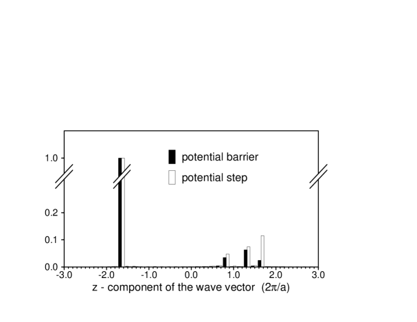
FIG. 2.: Comparison of grid calculations with a step potential and a potential barrier: modulus of the Fourier amplitudes normal to the surface in vacuum at $(x,y)=(0,0)$. The squared amplitudes give the LEED-intensities.

FIG. 3.: Comparison of the wave functions from a step potential and a potential barrier at $(x,y)=(0,0)$. The position of the step is indicated by the arrow.

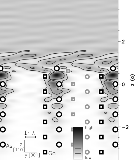
FIG. 4.: Gray scale image and contour plot of the charge density in the $yz$ plane at $x\!=\!0$ with a $z$ interval from $-3.55a$ to $3.95a$. In the $y$ direction two unit cells are shown. The atoms lying in the plane are drawn black, and in the right cell the projected positions of the remaining atoms are gray. The different scales for the $y$ and $z$ directions are indicated by the Ångstrøm scale.

REFERENCES

- [1] Present address: Fritz-Haber-Institut der Max-Planck-Gesellschaft, Faradayweg 4-6, D-14195 Berlin, Germany.
- [2] J. V. Peetz and W. Schattke, J. Electron Spectrosc. Relat. Phenom. 68, 167 (1994); M. Graß, J. Braun, and G. Borstel, Surf. Sci. 334, 215 (1995); O. Rubner, M. Kottcke, and K. Heinz, ibid. 340, 172 (1995).
- [3] J. B. Pendry, J. Phys. C 2, 2273 (1969)
- [4] P. M. Marcus and D. W. Jepsen, Phys. Rev. Lett. 20, 925 (1968).
- [5] G. Wachutka, Ph.D. thesis, Universityt München 1985.
- [6] G. Wachutka, Phys. Rev. B 34, 8512 (1986); Ann. Phys. (N.Y.) 187, 269 (1988); 187, 314 (1988).
- [7] Y. Joly, Phys. Rev. Lett. 68, 950 (1992); 72, 392 (1994); Phys. Rev. B 53, 13 029 (1996).
- [8] C. S. Lent and D. J. Kirkner, J. Appl. Phys. 67, 6353 (1990).
- [9] J. R. Chelikowsky, N. Troullier, and Y. Saad, Phys. Rev. Lett. 72, 1240 (1994); J. R. Chelikowsky, N. Troullier, K. Wu, and Y. Saad, Phys. Rev. B 50, 11 355 (1994).
- [10] J. Henk, W. Schattke, H. Carstensen, R. Manzke, and M. Skibowski, Phys. Rev. B 47, 2251 (1993).
- [11] W. Hackbusch, Multigrid Methods and Applications (Springer, Berlin, 1985).
- [12] E. L. Briggs, D. J. Sullivan, and J. Bernholc, Phys. Rev. B 52, R5471 (1995); 54, 14 362 (1996).