Strong Electron Tunneling through Mesoscopic Metallic Grains

Abstract

We describe electron transport through small metallic grains with Coulomb blockade effects beyond the perturbative regime. For this purpose we study the real-time evolution of the reduced density matrix of the system. In the first part of the paper we present a diagrammatic expansion for not too high junction conductance, $h/4\pi^{2}e^{2}R_{\rm t}\lesssim 1$, in a basis of charge states. Quantum fluctuations renormalize system parameters and lead to finite lifetime broadening in the gate-voltage dependent differential conductance. We derive analytic results for the spectral density and the conductance in the limit where only two charge states play a role. In the second part of the paper we consider junctions with large conductance, $h/4e^{2}R_{\rm t}\gtrsim 1$. In this case contributions from all charge states, which broaden and overlap, become important. We analyze the problem in a quasiclassical approximation. The two complementary approaches cover the essential features of electron tunneling for all parameters.

I Introduction

Electron transport through mesoscopic grains is strongly influenced by the large charging energy, $E_{\rm C}=e^{2}/2C$, associated with the low capacitance $C$ of the system [1, 2, 3, 4]. An interesting example is the “single-electron transistor” where a small metallic island is coupled via tunnel junctions to leads and via a capacitor to a gate voltage. At low temperatures, $T\ll E_{\rm C}$, a variety of single-electron phenomena have been observed in this system, including the Coulomb blockade and oscillations of the conductance as a function of a gate voltage. If the dimensionless conductance of the tunnel junctions between the island and the lead electrodes,

$$\alpha_{\rm t}\equiv\frac{R_{\rm K}}{4\pi^{2}R_{\rm t}}=\frac{h}{4\pi^{2}e^{2}R_{\rm t}}\,,$$ (1)

is small, on a scale defined by the quantum resistance $R_{\rm K}\simeq 25.8$ k$\Omega$, the charge of each island is a well-defined variable. In the limit $\alpha_{\rm t}\ll 1$, the sequential single-electron tunneling can be studied in perturbation theory [1, 3]; and descriptions based on a master equation or equivalent simulations of the stochastic dynamics are sufficient to account for the dominant features observed in single-electron devices.

Recent experiments beyond the perturbative regime show deviations from the classical description, e.g. a broadening of the conductance peaks much larger than temperature [5, 6]. This indicates that, in general, quantum fluctuations and higher-order coherent processes should be considered. Even in the limit of weak tunneling, $\alpha_{\rm t}<1$, nontrivial features appear in the vicinity of the Coulomb blockade threshold, when two charge states become nearly degenerate and perturbation theory fails. Several theoretical papers [8, 9, 10, 11, 12, 13, 14] dealt with the problem of higher-order processes, exploiting the physical picture of electron tunneling via discrete charge states. This includes “inelastic cotunneling” [7, 14], where in a second-order process in the parameter $\alpha_{\rm t}$ electrons tunnel via a virtual state of the island. An extension of this process, which gains importance near resonances, is “inelastic resonant tunneling” [10, 13], a process where electrons tunnel an arbitrary number of times between the reservoirs and the islands. The term “inelastic” indicates that with overwhelming probability different electron states are involved in the different steps of the higher order processes. The description can been extended to describe strong tunneling through single level quantum dots [15].

If the conductance of tunnel junctions is not small, $\alpha_{\rm t}\gtrsim 1$, the physical picture changes. In this case the inverse lifetime $\Gamma=1/R_{\rm t}C$ and, hence, the broadening of the excited charge states due to quantum fluctuations exceed the typical level spacing of excited island states, $\hbar\Gamma\gtrsim E_{\rm C}$. Thus charge levels overlap and the concept of tunneling via discrete charge states becomes ill-defined, raising the question whether charging effects survive under such conditions or whether they are washed out completely by strong quantum fluctuations. In Refs. [16, 17, 2, 18, 19, 12] it was demonstrated that at sufficiently low temperatures even for large values of $\alpha_{\rm t}$ quantum fluctuations of the charge do not destroy Coulomb blockade of tunneling, but they lead to a strong renormalization of the effective junction capacitance, $C_{\rm eff}\propto C\exp(2\pi^{2}\alpha_{\rm t})$. The exponential dependence on $\alpha_{\rm t}$ had been derived independently by renormalization group arguments [16, 12], instanton techniques [18], and Monte Carlo studies [12, 20]. One important consequence of the strong capacitance renormalization with increasing $\alpha_{\rm t}\gtrsim 1$ is the exponential reduction of the temperature limit below which charging effects can be observed.

This article is devoted to the calculation of the conductance of a SET transistor beyond perturbation theory in $\alpha_{\rm t}$, in a range of parameters which is accessible to experiments. The island contains a large number of electrons which are coupled strongly by Coulomb interactions. We, therefore, cannot proceed with ordinary perturbation theory. Rather, we reformulate the quantum mechanical many-body problem of these electrons in a real-time path-integral representation. In order to handle the Coulomb interaction we perform a Hubbard-Stratonovich transformation which introduces a phase as a collective variable. We trace out all microscopic degrees of freedom and arrive at an effective action of the system [21, 2], similar in structure to that known from the studies of Ohmic dissipation in quantum mechanics [22]. This procedure is addressed in Section 2.

After a change from the phase to a charge representation we are able to perform for $\alpha_{\rm t}\lesssim 1$ a diagrammatic expansion of the time evolution of the reduced density matrix. In a charge representation we can identify sequential, co- and resonant tunneling processes with certain classes of diagrams. A restriction to two charge states allows us to evaluate the spectral function and the conductance of the system analytically. The results will be presented in Section 3. At higher temperatures more charge states play a role, which in general requires a numerical study of the diagrammatic expansion.

In the opposite limit of strong tunneling, $\alpha_{\rm t}\gtrsim 1$, many charge states play a role, and a formulation in terms of the phase, which is canonically conjugated to the charge, is more convenient. This limit is discussed in Section 4. We analyze quantum dynamics of the phase variable in a semiclassical (saddle-point) approximation and obtain an expression for the system conductance valid at not too low temperatures $T\gtrsim e^{2}/2C_{\rm eff}$. The exponential renormalization of the effective capacitance for strong tunneling widens this temperature range substantially. The two approaches cover the essential features of electron tunneling for all parameters.

In Section 5 we review briefly some results obtained earlier within different imaginary time techniques, e.g. renormalization group and instanton methods, and compare these results with those of our real time analysis.

II Formulation of the Problem

We consider a metallic island coupled by two tunnel junctions (L,R) to two leads and capacitively to an external gate voltage $V_{\rm g}$. An applied transport voltage $V=V_{\rm L}-V_{\rm R}$ drives a current. A microscopic description of this single-electron transistor is based on the Hamiltonian, $H=H_{\rm L}+H_{\rm R}+H_{\rm I}+H_{\rm ch}+H_{\rm t,L}+H_{\rm t,R}$. Here $H_{\rm r}=\sum\limits_{k\sigma}\epsilon_{k\sigma{\rm r}}a^{\dagger}_{k\sigma{\rm r}}a_{k\sigma{\rm r}}$ describes noninteracting electrons in the left and right lead, r= L,R, and $H_{\rm I}=\sum\limits_{q\sigma}\epsilon_{q\sigma}c^{\dagger}_{q\sigma}c_{q\sigma}$ models the island states. The Coulomb interaction is accounted for in a capacitance model

$$H_{\rm ch}=E_{\rm C}\left(\sum\limits_{q\sigma}c^{\dagger}_{q\sigma}c_{q\sigma}-n_{\rm g}\right)^{2}\;.$$ (2)

The energy scale $E_{\rm C}\equiv e^{2}/(2C)$ of the transistor depends on the total island capacitance, $C=C_{\rm L}+C_{\rm R}+C_{\rm g}$, determined by the left and right tunnel junction and the gate capacitance. The charging energy can be tuned continuously by the “gate charge”

$$Q_{\rm g}\equiv-en_{\rm g}=-(C_{\rm L}V_{\rm L}+C_{\rm R}V_{\rm R}+C_{\rm g}V_{\rm g})\;.$$ (3)

The tunneling Hamiltonian $H_{\rm t,r}=\sum\limits_{kq\sigma}\left(T^{\sigma{\rm r}}a^{\dagger}_{k\sigma{\rm r}}c_{q\sigma}+{\rm h.c.}\right)$ describes tunneling between the island and the left and right leads. The matrix elements are related to the tunnel conductances by $R_{\rm r}^{-1}=(e^{2}/h)\sum\limits_{\sigma}N_{\rm r}^{\sigma}(0)N_{\rm I}^{\sigma}(0)|T^{\sigma{\rm r}}|^{2}$, where $N(0)$ denotes the densities of states of the island and the leads, respectively. In the following we will consider “wide” metallic junctions with $N\gg 1$ transverse channels. Extending the spin summation they can be labeled by the index $\sigma=1,...N$. In the following we will put $\hbar=1$ (except when it enters the quantum of resistance).

Our aim is to study the time-evolution of the density matrix. We shortly sketch the main steps of the derivation of this description:
– The time evolution of the density matrix introduces two propagators, a forward and backward propagator, which get coupled when we trace out electron degrees of freedom of the reservoirs. The procedure is known from the work of Caldeira and Leggett [22] who, generalizing earlier work of Feynman and Vernon, studied the influence of Ohmic dissipation on a quantum system. Similarly the influence on electron tunneling was described in Refs. [21, 2]. Here, we generalize the later work from a single tunnel junction to the transistor.
– In order to describe the Coulomb interaction between electrons we introduce via a Hubbard-Stratonovich transformation the electric potential of the island $V(t)$ as a macroscopic field. The interaction between electrons is replaced in this way by an interaction with the collective variable.
– We treat the leads as well as the electrons in the island as large equilibrium reservoirs. The electrochemical potentials of the reservoirs are fixed, $\mu_{\rm r}=-eV_{\rm r}$ for r = L,R. The only fluctuating field is voltage of the island $V(t)$. The definition $eV(t)\equiv-\dot{\varphi}(t)$ relates $V(t)$ to a phase $\varphi(t)$. Its quantum mechanical conjugate is the number of excess electrons $n(t)$ on the island. As a consequence of the procedure outlined so far, the macroscopic field $n(t)$ is independent of the microscopic degrees of freedom described by $c_{q\sigma}$ and $c^{\dagger}_{q\sigma}$. At this stage, the electronic degrees of freedom can be traced out.
– The time evolution of the reduced density matrix $\rho(t;\varphi_{1},\varphi_{2})$, which depends only on the phase variable $\varphi$, can thus be expressed by a double path integral over the phases corresponding to the forward and backward propagators $\varphi_{j}$ ($j=1,2$)

$$\rho_{\rm c}(t_{\rm f};\varphi_{\rm 1f},\varphi_{\rm 2f})=\int\limits_{-\infty}^{\infty}d\varphi_{\rm 1i}\int\limits_{-\infty}^{\infty}d\varphi_{\rm 2i}\int\limits_{\varphi_{\rm 1i}}^{\varphi_{\rm 1f}}{\cal D}[\varphi_{1}(t)]\int\limits_{\varphi_{\rm 2i}}^{\varphi_{\rm 2f}}{\cal D}[\varphi_{2}(t)]\exp\left(iS[\varphi_{1}(t),\varphi_{2}(t)]\right)\rho_{\rm c}(t_{\rm i};\varphi_{\rm 1i},\varphi_{\rm 2i})\,.$$ (4)

– The form (4) describes the situation where charges can take any continuous value and the phase is an extended variable. However, in our physical system the charge on the island is quantized in units of the electron charge $e$. In this case the phase variable is compact (i.e., the states $\varphi$ and $\varphi+2\pi$ are equivalent), and we rewrite (4), introducing integer winding numbers $m_{1},m_{2}=0,\pm 1,\pm 2,\dots$,

$$\rho_{\rm d}(t_{\rm f};\varphi_{\rm 1f},\varphi_{\rm 2f})=\sum\limits_{m_{1},m_{2}}\int\limits_{-\infty}^{\infty}d\varphi_{\rm 1i}\int\limits_{-\infty}^{\infty}d\varphi_{\rm 2i}\int\limits_{\varphi_{\rm 1i}}^{\varphi_{\rm 1f}+2\pi m_{1}}{\cal D}[\varphi_{1}(t)]\int\limits_{\varphi_{\rm 2i}}^{\varphi_{\rm 2f}+2\pi m_{2}}{\cal D}[\varphi_{2}(t)]$$ (5)

$$\exp\left(iS[\varphi_{1}(t),\varphi_{2}(t)]\right)\rho_{\rm d}(t_{\rm i};\varphi_{\rm 1i},\varphi_{\rm 2i})\,.$$ (6)

The two integrations can be combined to a single integral along the Keldysh contour, which runs forward and backward between $t_{\rm i}$ and $t_{\rm f}$ along the real-time axis. As a result the reduced propagator $\Pi$ is written as a single path integral along this contour

$$\Pi=\mbox{tr}\left[\rho_{0}\,T_{\rm K}\exp\left(-i\int_{\rm K}{\rm d}t\,H(t)\right)\right]=\int{\cal D}[\varphi(t)]\exp\left(iS[\varphi(t)]\right).$$ (7)

Here the collective variable $\varphi(t)$ and the time integral are defined on the Keldysh contour K, and the time-ordering operator $T_{\rm K}$ orders the following operators accordingly.

The effective action entering the propagator is $S[\varphi(t)]=S_{\rm ch}[\varphi(t)]+S_{\rm t}[\varphi(t)]$. The first term represents the charging energy

$$S_{\rm ch}[\varphi(t)]=\int_{\rm K}{\rm d}t\left[{C\over 2}\left({\dot{\varphi}(t)\over e}\right)^{2}+n_{\rm g}\dot{\varphi}(t)\right]\;.$$ (8)

Electron tunneling is described by $S_{\rm t}[\varphi(t)]$, which, in the case of wide metallic junctions, is expressed by the simplest electron loop connecting two times,

$$S_{\rm t}[\varphi(t)]=2\pi{\rm i}\sum\limits_{\rm r=L,R}\int_{\rm K}{\rm d}t\int_{\rm K}dt^{\prime}\alpha^{\rm K}_{\rm r}(t,t^{\prime}){\rm e}^{i\varphi(t)}{\rm e}^{-i\varphi(t^{\prime})}\;.$$ (9)

The kernels $\alpha^{\rm K}_{\rm r}(t,t^{\prime})=\alpha^{\pm}_{\rm r}(t-t^{\prime})$ for $t<t^{\prime}$ ($t>t^{\prime}$) depend on the order of the times along the Keldysh contour. Their Fourier transforms are [2, 10, 13]

$$\alpha^{\pm}_{\rm r}(\omega)=\pm\alpha_{\rm t,r}\frac{\omega-\mu_{\rm r}}{\exp[\pm(\omega-\mu_{\rm r})/T]-1}\,.$$ (10)

They are proportional to the dimensionless tunneling conductance $\alpha_{\rm t,r}=h/(4\pi^{2}e^{2}R_{\rm r})$ between the island and the leads r = L,R.

For large systems, the phase behaves almost like a classical variable while its conjugate variable, the charge, fluctuates strongly. A natural basis is then the phase representation. In the presence of strong Coulomb interaction, however, the situation is different: the phase underlies strong fluctuations while the time evolution of the charge is almost governed by classical rates. For this reason, it may be useful to change from the phase to the charge representation. The time evolution of the density matrix in a charge representation depends on the propagator from $n_{1}$ forward to $n_{1}^{\prime}$ and on the backward branch from $n_{2}^{\prime}$ backward to $n_{2}$. It is given by the matrix element of the reduced propagator [13]

$$\!\!\!\!\!\!\!\!\!\!\!\!\!\!\!\!\Pi^{n_{1},n_{1}^{\prime}}_{n_{2},n_{2}^{\prime}}=\int d\varphi_{1}\int d\varphi_{1}^{\prime}\int d\varphi_{2}^{\prime}\int d\varphi_{2}\,{\rm e}^{in_{1}\varphi_{1}}{\rm e}^{-in_{1}^{\prime}\varphi_{1}^{\prime}}{\rm e}^{in_{2}^{\prime}\varphi_{2}^{\prime}}{\rm e}^{-in_{2}\varphi_{2}}$$ (11)

$$\int\limits^{\varphi_{1},\varphi_{1}^{\prime}}_{\varphi_{2},\varphi_{2}^{\prime}}{\cal D}[\varphi(t)]\int{\cal D}[n(t)]\exp\left(-iS_{\rm ch}[n(t)]+iS_{\rm t}[\varphi(t)]+i\int_{\rm K}{\rm d}t\,n(t)\dot{\varphi}(t)\right)\,.\!\!\!\!\!\!\!$$ (12)

In the charge representation the charging energy is simply described by $S_{\rm ch}[n(t)]=\int_{\rm K}{\rm d}t\,E_{\rm C}\left[n(t)-n_{\rm g}\right]^{2}$.

III Expansion in the tunneling conductance

A diagrammatic description is obtained by expanding the tunneling term $\exp\left(iS_{\rm t}[\varphi(t)]\right)$ in the reduced propagator and integrating over $\varphi$. Each of the exponentials $\exp[\pm i\varphi(t)]$ describes tunneling of an electron at time $t$. These changes occur in pairs in each junction, r=L,R, and are connected by tunneling lines $\alpha^{\rm K}_{\rm r}(t,t^{\prime})$. Each term of the expansion can be visualized by a diagram. Several examples are displayed in Fig. 1. The value of a diagram is calculated according the rules which follow from the expansion of Eq. (11) and are presented in detail in Ref. [13].

The propagator from a diagonal state $n$ to another diagonal state $n^{\prime}$ is denoted by $\Pi^{n,n^{\prime}}_{n,n^{\prime}}=\Pi_{n,n^{\prime}}$. It is the sum of all diagrams with the given states at the ends and can be expressed by an irreducible self-energy part $\Sigma_{n,n^{\prime}}$, defined as the sum of all diagrams in which any vertical line cutting through them crosses at least one tunneling line. The propagator can be expressed as an iteration in the style of a Dyson equation, $\Pi_{n,n^{\prime}}=\Pi^{(0)}_{n}\delta_{n,n^{\prime}}+\sum\limits_{n^{\prime\prime}}\Pi_{n,n^{\prime\prime}}\,\Sigma_{n^{\prime\prime},n^{\prime}}\,\Pi^{(0)}_{n^{\prime}}$. The term $\Pi^{(0)}$ describes a propagation in a diagonal state which does not contain a tunneling line. The stationary probability for state $n$ follows from $P_{n}=\sum\limits_{n^{\prime}}P^{(0)}_{n^{\prime}}\,\Pi_{n^{\prime},n}$ (in which $P^{(0)}_{n}$ is the initial distribution) and is not the equilibrium one if a bias voltage is applied. Our diagram rules then yield

$$0=\sum\limits_{n^{\prime}}[-P_{n}\Sigma_{n,n^{\prime}}+P_{n^{\prime}}\Sigma_{n^{\prime},n}]\,.$$ (13)

We recover the structure of a stationary master equation with transition rates given by $\Sigma_{n^{\prime},n}$. In general, the irreducible self-energy $\Sigma$ yields the rate of all possible correlated tunneling processes. We reproduce the well-known single-electron tunneling rates by evaluating all diagrams which contain no overlapping tunneling lines. Similarly cotunneling is described by the diagrams where two tunneling lines overlapping in time, as shown in Fig. 1.

We calculate the current $I_{\rm r}$ flowing into reservoir ${\rm r=L,R}$ by adding a source term to the Hamiltonian and then taking the functional derivative of the reduced propagator with respect to the source. The result $I_{\rm r}=-ie\int d\omega\left\{\alpha_{\rm r}^{+}(\omega)C^{>}(\omega)+\alpha_{\rm r}^{-}(\omega)C^{<}(\omega)\right\}$ is expressed by the correlation functions $C^{>}(t,t^{\prime})=-i{\langle{\rm e}^{-i\varphi(t)}{\rm e}^{i\varphi(t^{\prime})}\rangle}$ and $C^{<}(t,t^{\prime})=i{\langle{\rm e}^{i\varphi(t^{\prime})}{\rm e}^{-i\varphi(t)}\rangle}$ describing charge transfer at different times. These are related to the spectral density for charge excitations on the island by $2\pi{\rm i}A(\omega)=C^{<}(\omega)-C^{>}(\omega)$.

For sequential tunneling, the current reduces to

$$I_{\rm r}={e\over h}4\pi^{2}\int d\omega\sum\limits_{\rm r^{\prime}}{\alpha_{\rm r^{\prime}}(\omega)\alpha_{\rm r}(\omega)\over\alpha(\omega)}A(\omega)[f(\omega-\mu_{\rm r^{\prime}})-f(\omega-\mu_{\rm r})]$$ (14)

with

$$A^{(0)}(\omega)=\sum\limits_{n=-\infty}^{\infty}[P_{n}+P_{n+1}]\delta(\omega-\Delta_{n})$$ (15)

and $\Delta_{n}=E_{\rm ch}(n+1)-E_{\rm ch}(n)=E_{\rm C}[1+2(n-n_{\rm g})]$.

At the minima of the Coulomb oscillations the system is in the Coulomb blockade regime, and cotunneling processes determine the conductance. The second order processes are described by diagrams as shown in Fig. 1. A careful analysis of our diagrammatic expansion not only reproduces the known limits [7] but also provides the needed regularization of divergences. We, furthermore, obtain new terms which are essential at the resonance. These results will be presented in a forthcoming publication [14].

At the resonance we have to include processes of arbitrary high order, since the process of resonant tunneling is essential. For definiteness, we concentrate on situations where only two charge states, $n=0,1$, need to be considered. This is the case when the energy difference of the two states $\Delta_{0}\equiv E_{\rm ch}(1)-E_{\rm ch}(0)$, the bias voltage $eV=eV_{\rm L}-eV_{\rm R}$, and the temperature $T$ are low compared to $E_{\rm C}$. If, furthermore, we restrict ourselves to matrix elements of the density matrix which are at most two-fold off-diagonal [13], we can evaluate – in a conserving approximation – the irreducible self-energy analytically. The following results are derived in this limit.

Using the notations $\alpha_{\rm r}(\omega)=\alpha^{+}_{\rm r}(\omega)+\alpha^{-}_{\rm r}(\omega)$ and $\alpha(\omega)=\sum\limits_{\rm r}\alpha_{\rm r}(\omega)$, we find $P_{0}=\lambda_{-}$ and $P_{1}=\lambda_{+}$ with $\lambda_{\pm}=\int d\omega\,\alpha^{\pm}(\omega)|\pi(\omega)|^{2}$ and

$$\pi(\omega)=[\omega-\Delta_{0}-\sigma(\omega)]^{-1}\qquad\!\!,\qquad\!\!\sigma(\omega)=\int d\omega^{\prime}\,{\alpha(\omega^{\prime})\over\omega-\omega^{\prime}+i0^{+}}\,.$$ (16)

Again, the current is given by Eq. (14), but the spectral density becomes

$$A(\omega)={\alpha(\omega)\over[\omega-\Delta_{0}-\mbox{Re}\,\sigma(\omega)]^{2}+[\mbox{Im}\,\sigma(\omega)]^{2}}\,.$$ (17)

The following results depend on the parameter

$$\alpha_{\rm t}=\sum\limits_{\rm r}\alpha_{\rm t,r}=\frac{h}{4\pi^{2}R_{\rm t}},$$ (18)

which also defines the parallel tunneling conductance $1/R_{\rm t}=\sum\limits_{\rm r}1/R_{\rm r}$. In lowest order in $\alpha_{\rm t}$ we have $A^{(0)}(\omega)=\delta(\omega-\Delta_{0})$, and the classical result is recovered. In general, quantum fluctuations yield energy renormalization and broadening effects, which enter in the spectral density via the complex self-energy $\sigma(\omega)$ given in Eq. (16). In order to evaluate $\sigma(\omega)$ we introduce a Lorentzian cut-off which we choose equal to $E_{\rm C}$ (since the energy difference to charge states which are not taken into account here is of the order of the charging energy). In this case we find

$${\rm Re}\,\sigma(\omega)=-\sum\limits_{\rm r}\alpha_{\rm t,r}(\omega-\mu_{\rm r})\left[2\ln\left({E_{\rm C}\over 2\pi T}\right)-2{\rm Re}\,\Psi\left(i\,{\omega-\mu_{\rm r}\over 2\pi T}\right)\right]$$ (19)

and ${\rm Im}\,\sigma(\omega)=-\pi\alpha(\omega)$. The effect of the quantum fluctuations can be estimated from the spectral density in the limits $T\gg eV,|\omega|$ or $eV\gg T,|\omega|$. Then, the spectral density is

$$A(\omega)={Z^{2}\alpha(\omega)\over[\omega-Z\Delta_{0}]^{2}+[\pi Z\alpha(\omega)]^{2}}\,,$$ (20)

with

$$Z^{-1}=1+2\alpha_{\rm t}\ln({E_{\rm C}/\max\{eV/2,2\pi T\}}).$$ (21)

We observe a renormalization of $\Delta_{0}$ and $\alpha_{\rm t}$ by $Z$ and a broadening given by $\pi Z\alpha(\omega)$. From this result we conclude that lowest order perturbation theory is sufficient for $\alpha_{\rm t}\ln{(E_{\rm C}/\max\{eV/2,2\pi T\})}\ll 1$. At larger values, our results for resonant tunneling show clear deviations from sequential tunneling.

A pronounced signature of quantum fluctuations is contained in the differential conductance $G=\partial{I}/\partial{V}$. In Figs. 2 and 3 we present our results for the differential conductance in the linear response regime ($V=0$). They clearly display the effect of resonant tunneling:
– For comparison, we show on the left hand side of Fig. 2 plots which are obtained from the master equation description of sequential tunneling,

$${G(T,n_{\rm g})\over G_{\rm as}}=\frac{1}{\sum_{n}\exp\left[-{E_{\rm C}\over T}(n-n_{\rm g})^{2}\right]}\sum_{n=-\infty}^{\infty}\exp\left[-{E_{\rm C}\over T}(n-n_{\rm g})^{2}\right]\frac{{E_{\rm C}\over T}(1+2(n-n_{\rm g}))}{\exp\left[{E_{\rm C}\over T}(1+2(n-n_{\rm g}))\right]-1}\,.$$ (22)

The asymptotic high-temperature conductance is $G_{\rm as}=1/(R_{\rm L}+R_{\rm R})$. At low temperatures, when processes involving only two charge states dominate, the maximal classical conductance saturates at one half of the asymptotic conductances at high temperatures. The width of the peaks scale linearly with temperature.
– The situation changes when resonant tunneling processes are taken into account (see the plots on the right hand side of Fig. 2). The maximal conductance and the peak width are renormalized by $Z$ and $Z^{-1}$ which depend logarithmically on temperature. For this reason, the conductance peak does not reach one half of the high temperature limit and decreases with lower temperatures, while the peak width is increased compared to the lowest order perturbation theory result. For an estimate of the maximal conductance, we use can the spectral density in the form of Eq. (20) and perform the integral Eq. (14) analytically,

$${G_{\rm max}(T)\over G_{\rm as}}\approx Z\left[{1\over 2}-{1\over\pi}\arctan\left({(\pi Z\alpha_{\rm t})^{2}-1\over 2\pi Z\alpha_{\rm t}}\right)\right]\,.$$ (23)

(The results shown in Fig. (3), however, were obtained by numerical analysis based on Eq. (17).)

Recent experiments [5, 6] in systems with junctions with small barriers show, indeed, a broadening and decreasing height of the linear conductance peaks, which cannot be explained by thermal smearing and qualitatively agrees with our theory.

The effects of quantum fluctuations are even more pronounced in the nonlinear differential conductance when the transport voltage dominates over temperature. In Fig. 4 we compare the results of perturbation theory and resonant tunneling at $T=0$ assuming that for $eV<2E_{\rm C}$ only two charge states $n=0,1$ are involved.
– The sequential tunneling result for a symmetric transistor with $\alpha_{\rm t,L}=\alpha_{\rm t,R}$ and $C_{\rm L}=C_{\rm R}$ is

$${G(V,n_{\rm g})\over G_{\rm as}}=2{E_{\rm C}^{2}(1-2n_{\rm g})^{2}+(eV)^{2}/4\over(eV)^{2}}\,\,\Theta\left({eV\over 4E_{\rm C}}-\left|n_{\rm g}-{1\over 2}\right|\right)\;.$$ (24)

As a function of $n_{\rm g}$ it shows a series of structures of width $CV/e$ with vertical steps at its edges. The width scales linearly with bias voltage.
– Resonant tunneling leads to a renormalization of the height and width by $Z$ and $Z^{-1}$ respectively, which depends now logarithmically on the voltage (see Fig. 4). For this reason, the height of the structure is below the sequential tunneling result and further decreases at lower voltages, while the width is enhanced. Furthermore, the sharp edges are smeared out even in the absence of thermal fluctuations (since $T=0$).

IV strong tunneling

If the junction conductance is high and hence the fluctuations in the charge are strong the phase representation outlined above is a more suitable starting point for the analysis of the problem. It turns out that the dimensionless conductance appears in the form

$$\tilde{\alpha}_{\rm t}=\frac{h}{4e^{2}R_{t}}=\pi^{2}\alpha_{\rm t}\;,$$ (25)

which differs from the expansion parameter $\alpha_{\rm t}$ of the weak tunneling expansion by a factor $\pi^{2}$. The real-time path-integral technique discussed above provides an expression for the reduced density matrix $\rho(\varphi_{1},\varphi_{2})$. If the island charge can vary continuously the density matrix $\rho_{\rm c}(\varphi_{1},\varphi_{2})$ is given by Eq. (4). It obeys the standard normalization condition $\int\limits_{-\infty}^{+\infty}d\varphi\rho_{\rm c}(\varphi,\varphi)=1$ and its time evolution is governed by the action $S[\varphi(t)]=\int_{K}{\rm d}t{\frac{C}{2}}\left({\frac{\dot{\varphi}(t)}{e}}\right)^{2}+S_{\rm t}[\varphi(t)]$. In this case the charging energy does not depend on the gate charge. In the SET transistor, another physical situation is realized, where the island charge is discrete and quantized in units of $e$. This situation is described by the density matrix $\rho_{\rm d}(\varphi_{1},\varphi_{2})$, Eq. (6), with a compact phase variable [2]. The normalization of the density matrix (6) is given by $\int\limits_{-\pi}^{\pi}d\varphi\rho_{\rm d}(\varphi,\varphi)=1$. It is sensitive to the gate charge. The comparison of Eq. (4) and (6) shows the following relation

$$\rho_{\rm d}(\varphi,\varphi)=A^{-1}\sum\limits_{m_{1},m_{2}}{\rm e}^{i2\pi n_{\rm g}(m_{1}-m_{2})}\rho_{\rm c}(\varphi+2\pi m_{1},\varphi+2\pi m_{2})\;.$$ (26)

Here $A$ is a normalization factor $A=\sum\limits_{m}\int\limits_{-\infty}^{+\infty}d\varphi{\rm e}^{i2\pi n_{\rm g}m}\rho_{\rm c}(\varphi+2\pi m,\varphi)$. The relation (26) can also be used to establish the connection between the expectation values of physical quantities for systems with discrete and continuous charge distributions. The expectation value of an operator $\hat{O}(\hat{\varphi})$, of the discrete-charge system, which is $2\pi$-periodic in $\varphi$ is

$$\left\langle\hat{O}\right\rangle_{\rm d} = \int\limits_{-\pi}^{\pi}d\varphi O(\varphi)\rho_{\rm d}(\varphi,\varphi)=\sum\limits_{m}\int\limits_{-\infty}^{+\infty}d\varphi O(\varphi){\rm e}^{i2\pi n_{\rm g}m}\rho_{\rm c}(\varphi-2\pi m,\varphi)$$ (27)

$$= \frac{\sum\limits_{m}\left\langle\hat{O}(\hat{\varphi}){\rm e}^{i2\pi(n_{\rm g}-\hat{n})m}\right\rangle_{\rm c}}{\sum\limits_{m}\left\langle{\rm e}^{i2\pi(n_{\rm g}-\hat{n})m}\right\rangle_{\rm c}}.$$ (28)

Here we used an obvious identity $\int d\varphi(...)\rho_{\rm c}(\varphi-2\pi m,\varphi)=\langle(...){\rm e}^{-2\pi{\rm i}\hat{n}m}\rangle_{\rm c}$.

Now we are ready to evaluate the tunneling current through a SET transistor. We first derive an expression for the expectation value of the current and then evaluate it with the aid of Eq. (28). The first part of this program will be carried out within the quasiclassical Langevin equation approach [21, 23, 24, 25, 26] derived under the assumption that fluctuations of the phase variable are weak. This assumption is justified if the fluctuations of the charges are strong.

In a semiclassical approximation we find for the current through the the left and the right junctions ${\rm r=L,R}$ (see Refs. [21, 24] for further details)

$$i_{\rm r}=C_{\rm r}\frac{\ddot{\varphi}_{\rm r}}{e}+\frac{1}{R_{\rm r}}\frac{\dot{\varphi}_{\rm r}}{e}-\tilde{\xi}_{r}(\varphi)\;.$$ (29)

It depends on the fluctuating voltage differences across the junctions, $\dot{\varphi}_{\rm r}/e=U-V_{\rm r}$ for ${\rm r}=1,2$. Here $U$ is the voltage of the island. Each current is the sum of displacement current on the capacitor, a deterministic tunneling current and a shot noise contribution. The latter can be expressed as a state-dependent noise in the form [21]

$$\tilde{\xi}_{\rm r}=\xi_{\rm r1}(t)\cos\varphi_{\rm r}+\xi_{\rm r2}(t)\sin\varphi_{\rm r}\;,$$ (30)

where $\xi_{{\rm r}i}$ ($i=1,2$) are two independent Gaussian stochastic variables with correlators

$$\left\langle\xi_{{\rm r}i}(0)\xi_{{\rm r}^{\prime}j}(t)\right\rangle=\delta_{\rm r,r^{\prime}}\delta_{i,j}\frac{1}{R_{\rm r}}\int\frac{d\omega}{2\pi}{\rm e}^{i\omega t}\omega\coth\left(\frac{\omega}{2T}\right).$$ (31)

We consider situations where the external impedance is negligible. In this case the phases $\varphi_{\rm r}$ are linked to the transport voltage $V$ by $\dot{\varphi}_{\rm L}-\dot{\varphi}_{\rm R}=eV$. We can further assume a symmetric bias $V_{\rm L}=-V_{\rm R}=V/2$. In this case the voltage on the island can be expressed as $U=(\dot{\varphi}_{\rm L}+\dot{\varphi}_{\rm R})/2e=V_{\rm g}+\dot{\varphi}_{\rm g}/e$. Here $\dot{\varphi}_{\rm g}/e$ is the voltage across the gate capacitance. Finally, charge conservation implies $i_{\rm L}+i_{\rm R}=-C_{\rm g}\ddot{\varphi}_{\rm g}/e$. Combining these relations with (29) we arrive, after averaging over the stochastic variables $\xi$, at the expression for the expectation value of the current

$$I=\langle i_{\rm L}\rangle=\frac{V-R_{\rm L}\left\langle\tilde{\xi}_{\rm L}\right\rangle_{\rm d}-R_{\rm R}\left\langle\tilde{\xi}_{\rm R}\right\rangle_{\rm d}}{R_{\rm L}+R_{\rm R}}\;.$$ (32)

This expression will be evaluated further with the aid of relation (28). If the fluctuations of the charge can be treated as Gaussian the contribution of the $m$-th winding number to the expectation value (28) can be estimated as

$$\left\langle\dots{\rm e}^{i2\pi\hat{n}m}\right\rangle_{\rm c}\sim\exp\left(-2\pi^{2}\left\langle\delta\hat{n}^{2}\right\rangle_{\rm c}m^{2}\right).$$ (33)

Thus provided that the charge fluctuations are not small $\left\langle\delta\hat{n}^{2}\right\rangle_{\rm c}\gtrsim 1$ it is sufficient to retain in the expression (28) only terms with winding numbers $m=0,\pm 1$. In this approximation we obtain [25]

$$\left\langle\tilde{\xi}_{\rm r}\right\rangle_{\rm d}=\frac{\ \left\langle\tilde{\xi}_{\rm r}\right\rangle_{\rm c}+2\left\langle\tilde{\xi}_{\rm r}\cos(2\pi(\hat{n}-n_{\rm g}))\right\rangle_{\rm c}}{1+2\left\langle\cos(2\pi(\hat{n}-n_{\rm g}))\right\rangle_{\rm c}}\;.$$ (34)

In the quasiclassical limit considered here the further analysis requires standard noise averaging of the solutions of Eqs. (29). As these equations are nonlinear in the phase, the exact solution cannot be constructed in general. In a wide parameter range, however, it is sufficient to proceed perturbatively in the noise terms. Making use of (32), (34) and assuming the phase fluctuations to be small $|\delta\varphi|\lesssim\pi$ we arrive at the following expression for the current

$$I(V)= G_{\rm as}V-I_{0}(V)$$ (36)

$$-{\rm e}^{-F(T,V)}\left[\left[I_{1}(V)-2I_{0}(V)\right]\cos\left(\frac{2\pi Q_{\rm av}(V)}{e}\right)+I_{2}(V)\sin\left(\frac{2\pi Q_{\rm av}(V)}{e}\right)\right],$$

Here

$$Q_{\rm av}=\langle e(\hat{n}-n_{\rm g})\rangle_{\rm c}=\frac{C_{\rm L}R_{\rm L}-C_{\rm R}R_{\rm R}}{R_{\rm L}+R_{\rm R}}V+C_{\rm g}V_{\rm g}$$ (37)

is the average charge of the metallic island. We further introduced the integrals

$$I_{0}(V)=\frac{2e}{\pi(R_{\rm L}+R_{\rm R})}\int\limits_{0}^{\infty}{\rm d}t\left(\frac{\pi T}{\sinh\pi Tt}\right)^{2}{\rm e}^{-W(t,V)}K(t)\cos\left(\frac{e(R_{\rm R}-R_{\rm L})Vt}{2(R_{\rm R}+R_{\rm L})}\right)\sin\left(\frac{eVt}{2}\right),$$ (38)

$$\begin{array}[]{c}I_{1}(V)\\ I_{2}(V)\end{array} = \frac{4e}{\pi(R_{\rm L}+R_{\rm R})}\int\limits_{0}^{\infty}{\rm d}t\left(\frac{\pi T}{\sinh\pi Tt}\right)^{2}{\rm e}^{-W(t,V)}\left[K(t)\begin{array}[]{c}\cosh\\ \sinh\end{array}(u(t,V))\right.$$ (48)

$$\left.+4\pi C\dot{K}(t)\begin{array}[]{c}\sinh\\ \cosh\end{array}(u(t,V))\right]\begin{array}[]{c}\cos\\ \sin\end{array}\left(\frac{e(R_{\rm R}-R_{\rm L})Vt}{2(R_{\rm R}+R_{\rm L})}\right)\sin\left(\frac{eVt}{2}\right)\;,$$

and we defined $K(t)=R_{t}\theta(t)(1-\exp(-t/R_{t}C))$, $1/R_{t}=1/R_{\rm L}+1/R_{\rm R}$ and

$$W(t,V)=-\frac{e^{2}}{2\pi}\int\limits_{-\infty}^{+\infty}dt_{1}\int\limits_{-\infty}^{+\infty}dt_{2}\left(\frac{\pi T}{\sinh\pi T(t_{1}-t_{2})}\right)^{2}K(t_{1},t)K(t_{2},t)$$ (49)

$$\sum\limits_{\rm r=L,R}\frac{1}{R_{\rm r}}\cos\left(\frac{eR_{\rm r}V(t_{1}-t_{2})}{R_{\rm L}+R_{\rm R}}\right),$$ (50)

with $K(t^{\prime},t)\equiv K(t^{\prime})-K(t^{\prime}-t)$. A principal value of the time integrals in (48), (50) should be taken where needed.

The function $F(T,V)=2\pi^{2}\langle\delta n^{2}\rangle$ determines the temperature and voltage dependence of the charge fluctuations in the Gaussian approximation. It is given by an expression similar to $W(t,V)$ (50) with the substitution $K(t_{1},t)K(t_{2},t)\to(4\pi^{2}C^{2}/e^{4})\dot{K}(t_{1})\dot{K}(t_{2})$. Analogously $u(t,V)$ is defined by (50) after the substitution $K(t_{1},t)\to-(4\pi C^{2}/e^{2})\dot{K}(t_{1})$.

We can simplify these expressions observing that in the limit of sufficiently high temperatures and/or voltages

$$\max\{eV,T\}\gg w_{0}=\frac{2\tilde{\alpha}_{\rm t}E_{\rm C}}{\pi^{2}}\exp(-2\tilde{\alpha}_{\rm t}+\gamma),\;\;\;$$ (51)

(here $\gamma=0.5772...$ is Euler’s constant) the results can be simplified further, since the time integration in (50) is effectively cut off at short times. Since $W(t=\min\{1/T,1/eV\},V)\ll 1$ we can set in the parameter range (51) in leading order approximation $W(t,V)=0$. With this simplification the above integrals can be evaluated analytically. We obtain

$$I_{0}(V)=\frac{eR_{0}}{R_{\rm L}+R_{\rm R}}\sum_{\rm r=L,R}\left\{\frac{eR_{\rm r}V}{\pi(R_{\rm L}+R_{\rm R})}\left[{\rm Re}\Psi\left(1+\frac{1}{2\pi TR_{0}C}-{\rm i}\frac{eR_{\rm r}V}{2\pi T(R_{\rm L}+R_{\rm R})}\right)\right.\right.$$ (52)

$$\left.\left.-{\rm Re}\Psi\left(1-{\rm i}\frac{eR_{\rm r}V}{2\pi T(R_{\rm L}+R_{\rm R})}\right)\right]\right\}$$ (53)

$$-\frac{1}{\pi R_{0}C}\sum\limits_{\rm r=L,R}{\rm Im}\Psi\left(1+\frac{1}{2\pi TR_{0}C}-{\rm i}\frac{eR_{\rm r}V}{2\pi T(R_{\rm L}+R_{\rm R})}\right)\;,$$ (54)

and

$$F(T,V) = F(0,0)+\frac{2\pi^{2}CT}{e^{2}}+\frac{2\pi}{e^{2}R_{0}}\ln\left(\frac{1}{2\pi TR_{0}C}\right)-$$ (56)

$$\frac{2\pi}{e^{2}}\sum\limits_{\rm r=L,R}{\rm Re}\left[\frac{1}{R_{\rm L}}\left(1-{\rm i}\frac{eR_{\rm r}R_{0}C}{R_{\rm L}+R_{\rm R}}V\right)\Psi\left(1+\frac{1}{2\pi TR_{0}C}-{\rm i}\frac{eR_{\rm r}V}{2\pi T(R_{\rm L}+R_{\rm R})}\right)\right]\;.$$

Here $\Psi(x)=\Gamma^{\prime}(x)/\Gamma(x)$ is the digamma function.

The last expression determines the temperature and voltage dependence of the charge fluctuations $\langle\delta n^{2}\rangle$ at not too low $T$ and/or $V$. At $T=0$ and $V=0$ the integral over time in $F(T,V)$ diverges logarithmically at high frequencies. This divergence indicates a failure of the quasiclassical Langevin equation in this limit. The problem can be cured by observing that in thermodynamic equilibrium (zero voltage) in Gaussian approximation

$${\rm e}^{-F(0,0)}=\left\langle\cos(2\pi\hat{n})\right\rangle=\frac{\int d\varphi\rho_{\text{eq}}(2\pi+\varphi,\varphi)}{\int d\varphi\rho_{\text{eq}}(\varphi,\varphi)}\;.$$ (57)

The expectation value involving the equilibrium density matrix can be evaluated [25] with the result

$$F(0,0)\simeq 2\tilde{\alpha}_{\rm t}\;.$$ (58)

The functions $I_{1}(V)$ and $I_{2}(V)$ cannot be evaluated analytically even in the limit (51). Due to a fast decay of the exponential factor $\exp[-F(T,V)]$ in (36) with increasing $V$ and $T$ it is sufficient to evaluate $I_{1}$ and $I_{2}$ in the low voltage and temperature limit. In this limit the integral (48) reduces to

$$I_{1}(V)-2I_{0}(V)\approx gG_{\rm as}V,\;\;\;g=\frac{1.22}{\tilde{\alpha}_{\rm t}}+11.29.$$ (59)

whereas the function $I_{2}(V)$ turns out to be small $I_{2}(V)\sim V^{2}\approx 0$ and will be neglected below.

We thus arrive at the following result for the I-V characteristics of a SET transistor

$$I(V)=G_{\rm as}V-I_{0}(V)-gG_{\rm as}V{\rm e}^{-F(T,V)}\cos\left(\frac{2\pi Q_{\rm av}(V)}{e}\right)\;.$$ (60)

The current is reduced below the classical result $G_{\rm as}V$ by an amount $I_{0}(V)$ and is modulated in a periodic way by the gate voltage. In the limit considered the modulation is a pure cos-modulation. The result (60) also describes the oscillatory behavior of the current as a function of the transport voltage, which is usually referred to as a “Coulomb staircase”. The amplitude of these oscillations decays exponentially with increasing voltage and temperature. We also recover the fact that the Coulomb staircase is pronounced only in asymmetric SET transistors. In a symmetric case the transport voltage drops out from the expression for the gate charge (3). The I-V characteristics (60) is depicted in Fig. 5 for different temperatures and values of the gate charge.

The linear conductance of a SET transistor can be easily derived from Eq. (60) in the limit $V\rightarrow 0$. We find

$${\frac{G(T)}{G_{\rm as}}}=1-f(T)-g{\rm e}^{-F(T,0)}\cos\left(2\pi n_{\rm g}\right)\;,$$ (61)

where $n_{\rm g}=C_{\rm g}V_{\rm g}/e$ and

$$f(T)=\frac{1}{2\tilde{\alpha}_{\rm t}}\left[\gamma+\frac{2\tilde{\alpha}_{\rm t}E_{\rm C}}{\pi^{2}T}\Psi^{{}^{\prime}}\left(1+\frac{2\tilde{\alpha}_{\rm t}E_{\rm C}}{\pi^{2}T}\right)+\Psi\left(1+\frac{2\tilde{\alpha}_{\rm t}E_{\rm C}}{\pi^{2}T}\right)\right]\;.$$ (62)

These results are displayed in Figs. 6 and  7 in the temperature range $T\gtrsim 10w_{0}$, where we estimate the approximations used above to be justified.

In the high-temperature limit the conductance becomes independent of the gate charge, but due to charging effects it is still reduced below the asymptotic value by

$${\frac{G(T)}{G_{\rm as}}}=1-\frac{E_{\rm C}}{3T}+\left(\frac{6\zeta(3)}{\pi^{4}}\tilde{\alpha}_{\rm t}+\kappa\right)\left(\frac{E_{\rm C}}{T}\right)^{2}-...$$ (63)

For high temperatures this expression is valid for all (including small) values of $\tilde{\alpha}_{\rm t}$. The first nontrivial term in this expansion does not depend on $\tilde{\alpha}_{\rm t}$. The coefficient of the square term also contains an $\tilde{\alpha}_{\rm t}$-independent contribution $\kappa$. Within the approximation $W=0$ used here we have $\kappa=0$. An improved approximation is obtained by expanding in $W(t,V)$, or alternatively by treating the general expression for the system conductance perturbatively in $\tilde{\alpha}_{\rm t}$ and then expanding in $E_{\rm C}/T$. This procedure yields $\kappa=1/15$, which for large $\tilde{\alpha}_{\rm t}$ can be neglected against the first term $6\zeta(3)\tilde{\alpha}_{\rm t}/\pi^{4}$.

At lower temperatures the conductance is further suppressed by charging effects and it can be modulated by the gate charge $Q_{\rm g}$. In the figures the minimum and maximum conductance values are presented corresponding to $Q_{\rm g}=0$ and $Q_{\rm g}=e/2$, as well as the $Q_{\rm g}$-averaged conductance. The modulation with $Q_{\rm g}$ becomes more pronounced as the temperature is lowered, however, it is exponentially suppressed with increasing $\tilde{\alpha}_{\rm t}$ (cf. Figs. 6 and  7). For $\tilde{\alpha}_{\rm t}\gtrsim 4$ the modulation effect can hardly be resolved while the overall suppression of the system conductance $G$ is very pronounced.

Although the validity of the Langevin description description is restricted to high temperatures and/or voltages, $T,eV\gg w_{0}$, the validity range rapidly expands as $\tilde{\alpha}_{\rm t}$ increases. E.g. for the parameters $E_{\rm C}\sim 1$ K and $\tilde{\alpha}_{\rm t}\approx 2$, we get $w_{0}$ in the range 15 mK. Further increase of $\tilde{\alpha}_{\rm t}$ rapidly brings $w_{0}$ below 1 mK. Therefore we can conclude that in the strong tunneling regime $\tilde{\alpha}_{\rm t}>2\div 3$ our theory covers the experimentally accessible temperatures. Indeed a quantitative agreement without fitting parameters exists between our results (61-63) and those of the Saclay group [5] in the high temperature regime. For lower temperatures the quasiclassical Langevin equation approach can be applied only to sample 4 of Ref. [5] with $\tilde{\alpha}_{\rm t}\simeq 1.8$. Other samples studied in Ref. [5] have substantially lower conductance, and their low-temperature behavior should be described by the expansion in $\alpha_{\rm t}$ presented in Section 3.

V Discussion

In a number of earlier papers [16, 18, 19, 12] the combination of charging and strong tunneling effects in metallic junctions has been analyzed within imaginary time approaches. In the limit of strong tunneling, $\tilde{\alpha}_{\rm t}\gg 1$, a renormalization group equation for $\tilde{\alpha}_{\rm t}$ can be derived [16, 2]

$$d\tilde{\alpha}_{\rm t}/d\ln\omega_{\rm c}=\beta(\tilde{\alpha}_{\rm t})\;,$$ (64)

where in the lowest order in $\tilde{\alpha}_{\rm t}$ one has $\beta(\tilde{\alpha}_{\rm t})=1/2$. Already this scaling approach captures the tendency of the effective junction conductance to decrease with decreasing $T$ due to charging effects. In order to see that one should proceed with scaling from $\omega_{\rm c}\sim E_{\rm C}$ to $\omega_{\rm C}\sim T$ and identify the (dimensionless) junction conductance with the renormalized value $\tilde{\alpha}_{\rm t}(\omega_{\rm c}\sim T)$. This approach is sufficient for strong tunneling at high temperatures, namely if the final renormalized tunneling conductance still satisfies $\tilde{\alpha}_{\rm t}(\omega_{\rm c}\sim T)\gtrsim 1$. In general the strong tunneling approach may lead to a small renormalized conductance such that (64) ceases to be valid. For weak tunneling other scaling approaches, derived in an expansion in the tunneling conductance and equivalent to what we described in Section III, can be applied. In this situation, Falci et al. [12] suggested a 2-stage scaling procedure, where the renormalized conductance after the strong tunneling rescaling was used as an entry parameter for the weak tunneling scaling.

Various theoretical approaches led to the conclusion the strong electron tunneling $\tilde{\alpha}_{\rm t}\gg 1$ reduces the charging energy, i.e. the effective capacitance is renormalized. Panyukov and Zaikin [18] treated the problem by means of instanton techniques. They concluded that electron tunneling affects both the scale and the functional dependence of the ground state energy $E(Q_{\rm g})$. At not too low temperatures $T\gtrsim w$ they find

$$E(Q_{\rm g})=-\frac{w}{2}\cos(\frac{2\pi Q_{\rm g}}{e})$$ (65)

with [18]

$$w=\frac{32\tilde{\alpha}_{\rm t}E_{\rm C}}{\pi^{2}}\exp(-2\tilde{\alpha}_{\rm t}+\gamma).$$ (66)

A similar result, differing only in the numerical coefficient, has been obtained in a semiclassical analysis of the effective action [12].

At lower temperatures the form of the lowest energy band $E(Q_{\rm g})$ turns out to be even more complicated [18, 12] and the $\tilde{\alpha}_{\rm t}$-dependence of the prefactor of the expression for $w$ changes from linear in $\tilde{\alpha}_{\rm t}$ for $T>w$ to quadratic in $\tilde{\alpha}_{\rm t}$ for $T=0$. Instanton techniques [18] yield

$$E_{\rm C,eff}\propto\alpha_{\rm t}^{2}E_{C}\exp(-2\tilde{\alpha}_{\rm t})\;.$$ (67)

The exponential dependence on $\alpha_{\rm t}$ has been confirmed by renormalization group arguments [16, 2, 12] as well as Monte Carlo methods [12, 20]. The prefactor remains a point of controversial discussions in the literature  [20]. Irrespective of this detail an important consequence of the strong capacitance renormalization for $\alpha_{\rm t}\gtrsim 1$ is the exponential reduction of the temperature range where charging effects are observable.

With the aid of relations (65), (66) we can derive the first order correction in $1/\tilde{\alpha}_{\rm t}$ in the renormalization group equation (64) [27]

$$\beta(\tilde{\alpha}_{\rm t})=1/2+1/4\tilde{\alpha}_{\rm t}.$$ (68)

This result has also been derived by direct RG methods [28].

A consequence of the renormalization group approach (64) has been pointed out in Ref. [18]. It relies on the assumption that the system linear conductance is determined by the renormalized value $\tilde{\alpha}_{\rm t}(\omega_{\rm c}\sim T)$ as

$$G=\frac{2e^{2}}{\pi\hbar}\tilde{\alpha}_{\rm t}(\omega_{\rm c}\sim T)\;.$$ (69)

Combining the above scaling approach, the high temperature expansion (63) (with $\kappa=0$), and the expression (68) for $\beta$ to first order in $1/\alpha_{\rm t}$ we get for the $Q_{\rm g}$-averaged conductance

$$\frac{G}{G_{\rm as}}=1-\frac{1}{2\tilde{\alpha}_{\rm t}}\left\{\ln\left(1+\frac{4\tilde{\alpha}_{\rm t}^{2}}{3(1+2\tilde{\alpha}_{\rm t})}\frac{E_{\rm c}}{T}\right)+\ln\left[1+\frac{1}{2\tilde{\alpha}_{\rm t}}\ln\left(1+\frac{4\tilde{\alpha}_{\rm t}^{2}}{3(1+2\tilde{\alpha}_{\rm t})}\frac{E_{\rm C}}{T}\right)\right]\right\}.$$ (70)

Although the above scaling approach to the conductance calculation is intuitively attractive (and the result (70) fits reasonably with the available experimental data [5, 6]) it has to be stressed that it depends on the unproven assumption (69).

In contrast, the real-time path-integral techniques presented here are free from this ambiguity and allow for a direct evaluation of the $I$-$V$ characteristics and the system conductance. We note, furthermore, that the results obtained within the real and imaginary time methods are consistent with each other. E.g. the renormalization of the effective energy difference between the two lowest charge states, derived in Ref. [12], is contained in the self-consistent solution presented in Section 3. Furthermore, comparing the expressions for $w_{0}$ (51) and the bandwidth $w$ (66) we immediately see that these two parameters coincide up to a numerical coefficient: $w=16w_{0}$. This means the requirement for the validity of the quasiclassical Langevin equation (51) roughly coincides with the requirement that the temperature (or voltage) is larger than the effective bandwidth $w$.

Still no quantitative theory for the conductance at lower temperatures and not too low values $\tilde{\alpha}_{\rm t}\gtrsim 1$ has been provided. Although the two limiting descriptions presented here do not allow for a quantitative description of this parameter range it satisfactory to notice that both show the same qualitative trend in this range.

Another question of interest is the conductance at very large $\tilde{\alpha}_{\rm t}\gg 1$ and very low $T\lesssim w_{0}$. In the limit $\tilde{\alpha}_{\rm t}\gg 1$ the conductance oscillations with $Q_{\rm g}$ are exponentially small (cf. (61)). Then for all $Q_{\rm g}$ from (61,58) we have

$$G(T\approx w_{0})/G_{as}\simeq b/\tilde{\alpha}_{\rm t},\;\;\;b\sim 1.$$ (71)

Thus we can conjecture that the low temperature maximum conductance of a SET transistor is universal in the limit of large $\tilde{\alpha}_{\rm t}$ being of the order of the inverse quantum resistance unit $2e^{2}/\pi\hbar$. This conjecture is also consistent with the scaling analysis of Refs. [16, 18, 12] combined with the results of Section 3. Starting from large $\tilde{\alpha}_{\rm t}\gg 1$ we first use the renormalization group procedure (64,68) which should be cut at $\tilde{\alpha}_{\rm t}(\omega_{\rm c})\sim 1$. In the second stage we expand in $\alpha_{\rm t}\approx 1/\pi^{2}$ as described in Section 3 – starting with the renormalized value instead of the bare one. Apart from logarithmic corrections we thus arrive at the maximum conductance of order of the inverse quantum resistance, no matter how large the initial conductance is.

VI Conclusions

In this paper we have described single-electron tunneling in systems with strong charging effects beyond perturbation theory in the tunneling conductance. For this purpose we considered the real-time evolution of the reduced density matrix of the system. We presented two approximation schemes:
In the first part, valid for not too strong tunneling, $\alpha_{{\rm t}}\lesssim 1$, we presented a systematic diagrammatic expansion, which allowed us to identify the different contributions, sequential tunneling, inelastic cotunneling and inelastic resonant tunneling. When we restricted ourselves to diagrams corresponding to maximally two-fold off-diagonal matrix elements of the density matrix we can formulate a self-consistent resummation of diagrams. At low temperatures we, furthermore, can restrict our attention to two consecutive charge states. In this limit, there exist no crossing diagrams, and we can evaluate the summation in closed form. The most important results are a renormalization of system parameters and a life-time broadening of the conductance peaks. These two approximations are justified for tunneling conductances satisfying $\alpha_{{\rm t}}\ln{(E_{{\rm C}}/\max\{eV/2,2\pi T\})}\lesssim 1$ and allow for a qualitative analysis of the system conductance also for larger values of $\alpha_{{\rm t}}$.

In the second part of the paper we developed an alternative approach based on quasiclassical Langevin equations for the junction phase $\varphi$. This approach assumes that fluctuations of the phase are small and that the noise can be treated perturbatively. This is a suitable approximation for large values $\tilde{\alpha}_{{\rm t}}=\pi^{2}\alpha_{{\rm t}}$ or in the high temperature limit. For weak tunneling $\tilde{\alpha}_{{\rm t}}\lesssim 1$ this scheme turns out to be justified only for high temperatures and/or voltages max$(T,eV)\gg E_{{\rm C}}$, whereas for stronger tunneling, $\tilde{\alpha}_{{\rm t}}\gtrsim 1$, phase fluctuations are substantially suppressed. The results derived in this approach are valid, provided max$\{T,eV\}\gg\tilde{\alpha}_{{\rm t}}E_{{\rm C}}\exp(-2\tilde{\alpha}_{{\rm t}})$. This range expands rapidly with increasing $\tilde{\alpha}_{{\rm t}}$.

In conclusion, we found an effective action description of a single-electron transistor. We analyzed it in two limits. The charge representation, which is valid as long as $\alpha_{{\rm t}}\lesssim 1$, provides the basis for a systematic diagrammatic description of coherent tunneling processes including resonant tunneling. The phase representation is suitable at large values of $\tilde{\alpha}_{{\rm t}}\gtrsim 1$. In both cases we calculated the gate-voltage and temperature-dependent conductance of a single electron transistor. The dimensionless parameters in the two limits differ by a factor $\pi^{2}\alpha_{{\rm t}}=\tilde{\alpha}_{{\rm t}}$. As a result the range of validity of the two approaches overlaps and, at least qualitatively, the two approaches cover the whole range of parameters.

The authors are grateful to D. Esteve, G. Falci and G.T. Zimanyi for useful discussions. We thank the members of the Saclay group for sending us their data prior to publication. The project was supported by the DFG within the research program of the Sonderforschungbereich 195 and by INTAS-RFBR Grant No. 95-1305.

FIG. 1.: A diagram showing from left to right: sequential tunneling in the left and right junction, a term preserving the norm, a cotunneling process, and resonant tunneling.

FIG. 2.: The linear differential conductance normalized to the high temperature limit. Left hand side: result from a master equation in lowest order perturbation theory with $T/E_{\rm C}=0.01,0.05,0.1,0.2,0.3,0.4,0.5,0.75,1,2,5$, and $10$. In this limit the scaled conductance is independent of $\alpha_{\rm t}$. Right hand side: result of resonant tunneling with $\alpha_{\rm t}=0.2$ and $T/E_{\rm C}=0.01,0.05$, and $0.1$.

FIG. 3.: The maximum linear differential conductance normalized to the high temperature limit for $\alpha_{\rm t}=0.001,0.01,0.1,0.2$ (from top to bottom). For comparison we also show the result obtained from lowest order perturbation theory (dashed line and inset).

FIG. 4.: The normalized nonlinear differential conductance for $\alpha_{\rm t}=0.1$ and $eV/E_{\rm C}=0.05,0.2,0.5$ at zero temperature. The inset shows the result from a master equation in lowest order perturbation theory for $eV/E_{\rm C}=0.5$.

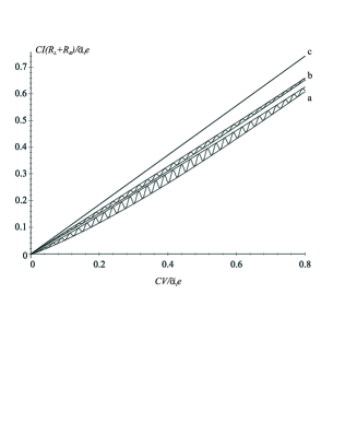
FIG. 5.: The current-voltage characteristics of a symmetric ($R_{\rm L}=R_{\rm R}$) SET transistor in the strong tunneling regime defined by eq. (60) at $\tilde{\alpha}_{\rm t}=2.5$ and different temperatures $T/\tilde{\alpha}_{\rm t}E_{\rm C}=$ 0.01 (a), 0.2 (b), and 1 (c). For each temperature maximum and minimum currents are plotted. Curves with oscillations demonstrate the gate modulation effect. This effect is completely suppressed in the high temperature limit (curve (c)).

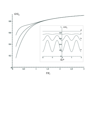
FIG. 6.: Maximum and minimum linear conductance of a SET transistor as a function of temperature obtained from the Langevin equation analysis (eq. (61)) for $\tilde{\alpha}_{\rm t}=2$. The intermediate curve shows the linear conductance averaged over all values of the gate charge. Inset: Conductance as a function of the gate charge for the same $\tilde{\alpha}_{\rm t}$ at different temperatures $T/E_{\rm C}=$ 0.15 (a), 0.5 (b), 1 (c) and 2 (d).

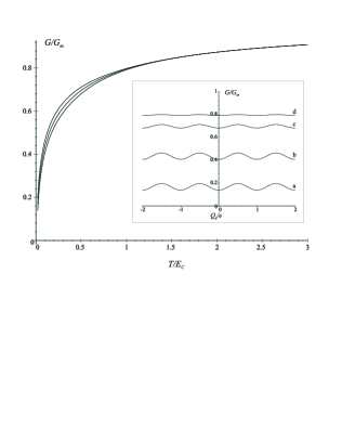
FIG. 7.: The same as in fig. 6 for $\tilde{\alpha}_{\rm t}=3$. The curves (a), (b), (c) and (d) in the inset correspond respectively to $T/E_{\rm C}=$ 0.02, 0.1, 0.5 and 1.

REFERENCES

- [1] D. V. Averin and K. K. Likharev, in Mesoscopic Phenomena in Solids, B. L. Altshuler, P. A. Lee and R. A. Webb, eds., p. 173 (Elsevier, Amsterdam, 1991).
- [2] G. Schön and A.D. Zaikin, Phys. Rep. 198, 237 (1990).
- [3] Single Charge Tunneling, NATO ASI Series, Vol. 294, edited by H. Grabert and M.H. Devoret, (Plenum Press), 1992.
- [4] Proceedings of the NATO ARW Mesoscopic Superconductivity, Physica B 203, Nos. 3, 4 (1994), edited by F.W.J. Hekking, G. Schön and D.V. Averin.
- [5] P. Joyez, V. Bouchiat, D. Estève, C. Urbina, and M.H. Devoret, submitted to Phys. Rev. Lett.
- [6] D. Chouvaev et al., in preparation.
- [7] D.V. Averin and Yu.V. Nazarov, in Ref. [3].
- [8] K.A.Matveev, Sov. Phys. JETP 72, 892 (1991).
-
[9]
D.S. Golubev and A.D. Zaikin, Phys. Rev. B 50, 8736
(1994);
A.D. Zaikin, D.S. Golubev, and S.V. Panyukov, in Ref. [4]. - [10] H. Schoeller and G. Schön, Phys. Rev. B 50, 18436 (1994), and also in Ref. [4].
- [11] H. Grabert, Phys. Rev. B 50, 17364 (1994).
- [12] G. Falci, G. Schön and G. T. Zimanyi, Phys. Rev. Lett. 74, 3257 (1995), and also in Ref. [4].
-
[13]
J. König, H. Schoeller, and G. Schön, Europhys. Lett. 31, 31
(1995);
J. König, H. Schoeller, G. Schön, and R. Fazio, in Quantum Dynamics of Submicron Structures, eds. H. A. Cerdeira et al., NATO ASI Series E, Vol. 291 (Kluwer, Dordrecht) 1995, p.221. - [14] J. König and H. Schoeller, preprint.
-
[15]
J. König, H. Schoeller, and G. Schön, Phys. Rev. Lett. 76, 1715
(1996);
J. König, J. Schmid, H. Schoeller, and G. Schön, Phys. Rev. B 54, 16820 (1996). - [16] F. Guinea, and G. Schön, Europhys. Lett. 1, 585 (1986); J. Low Temp. Phys. 69 219 (1987).
- [17] A.D. Zaikin, and S.V. Panyukov, Zh. Eksp. Teor. Fiz. 94, 172 (1988) [Sov. Phys. JETP 67, 2487 (1988)]; J. Low Temp. Phys. 73, 1 (1988).
- [18] S.V. Panyukov, and A.D. Zaikin, Phys. Rev. Lett. 67, 3168 (1991).
- [19] A.D. Zaikin and S.V. Panyukov, Phys. Lett. A 183, 115 (1993).
- [20] X. Wang, R. Egger, and H. Grabert, Czechoslovak Journal of Physics, 46, 2387 (1996); X. Wang and H. Grabert, Phys. Rev. B 53, 12621 (1996)
- [21] U. Eckern, G. Schön and V. Ambegaokar, Phys. Rev. B 30, 6419 (1984).
- [22] A.O. Caldeira and A.J. Leggett, Ann. Phys. (N.Y.) 149, 374 (1983).
- [23] A. Schmid, J. Low Temp. Phys. 49, 609 (1982).
- [24] D.S. Golubev and A.D. Zaikin, Phys. Rev. B 46, 10903 (1992); Phys. Lett. A 169, 337 (1992).
- [25] D.S. Golubev and A.D. Zaikin, Zh. Eksp. Teor. Fiz. Pis’ma Red. 63, 953 (1996) [JETP Lett. 63, 1007 (1996)].
- [26] See also an earlier paper by A.A. Odintsov, Zh. Eksp. Teor. Fiz. 94, 312 (1988) [Sov. Phys. JETP 67, 1265 (1988)] where the analogy with the polaron problem has been exploited and a similar approximation has been made.
- [27] In Ref. [18] the function was derived for a more general case of a tunnel junction interacting with a linear Ohmic dissipative environment.
- [28] W. Hofstetter and W. Zwerger, unpublished.