Scaling behavior in economics: II. Modeling of company growth

Abstract

In the preceding paper we presented empirical results describing the growth of publicly-traded United States manufacturing firms within the years 1974–1993. Our results suggest that the data can be described by a scaling approach. Here, we propose models that may lead to some insight into these phenomena. First, we study a model in which the growth rate of a company is affected by a tendency to retain an “optimal” size. That model leads to an exponential distribution of the logarithm of the growth rate in agreement with the empirical results. Then, we study a hierarchical tree-like model of a company that enables us to relate the two parameters of the model to the exponent $\beta$, which describes the dependence of the standard deviation of the distribution of growth rates on size. We find that $\beta=-\ln\Pi/\ln z$, where $z$ defines the mean branching ratio of the hierarchical tree and $\Pi$ is the probability that the lower levels follow the policy of higher levels in the hierarchy. We also study the distribution of growth rates of this hierarchical model. We find that the distribution is consistent with the exponential form found empirically.

I Introduction

The concept of scaling supports much of our current conceptualization on the general subject of how complex systems formed of interacting subunits behave. This concept was developed a quarter century ago by physicists interested in the behavior of a system near its critical point. Progress was made possible by a remarkable combination of experiment and phenomenological theory. In the preceding paper we presented empirical results suggesting that the scaling concept can be useful in describing economic systems [1, 2]. In this paper we present models which may lead to an understanding of the underlying mechanism behind the scaling laws.

In the preceding paper, we used the Compustat database to study all United States (US) manufacturing publicly-traded firms from 1974 to 1993. The Compustat database contains $20$ years of data on all publicly-traded companies in the US. We found that the distribution of firm sizes remains stable for the 20 years we study, i.e., the mean value and standard deviation remain approximately constant. We studied the distribution of sizes of the “new” companies in each year and found it to be well approximated by a log-normal. However, we find (i) the distribution of the logarithm of the growth rates, for a growth period of one year, and for companies with approximately the same size $S_{0}$ displays an exponential form [3, 4]

$$p(r_{1}|S_{0})=\frac{1}{\sqrt{2}\sigma_{1}(S_{0})}\exp\left(-{\frac{\sqrt{2}~{}|r_{1}-\bar{r}_{1}|}{\sigma_{1}(S_{0})}}\right)\,,$$ (1)

and (ii) the fluctuations in the growth rates — measured by the width of this distribution $\sigma_{1}$ — scale as a power law [4],

$$\sigma_{1}(S_{0})\sim{S_{0}}^{-\beta}\,.$$ (2)

Here $r_{1}=\ln(S_{1}/S_{0})$, where $S_{1}$ is the size of the company in the next year, and $\sigma_{1}(S_{0})$ is the standard deviation (width) of the distribution (1). We found that the exponent $\beta$ takes the same value, within the error bars, for several measures of the size of a company. In particular, we obtained: $\beta=0.20\pm 0.03$ for “sales.”

In this paper, we present and discuss models that, although very simple, give some insight into these empirical results. The paper is organized as follows. In Sect. II, we discuss a model that predicts an exponential distribution of growth rates. In Sect. III, we study a hierarchical tree model that predicts the power law dependence of $\sigma_{1}$ on size. In Sect. IV, we discuss how the two models can be combined so that a single model predicts both of our central empirical findings. In Sect. V, we summarize our findings and suggest avenues for future research. The paper contains three appendices. Appendix A discusses the relationship between the standard deviations of the growth rate and the logarithmic growth rate. Appendices B and C give more details of the analytical solution of the hierarchical tree model.

II The exponential distribution of growth rates

As described above, one of our central findings is that the distribution of growth rates for companies of a given initial size has an exponential form. The result is surprising because the sales of organizations as large as publicly traded corporations reflect a large number of factors. While those factors are not necessarily independent and while the growth of any one company might be dominated by a single factor, one might nonetheless expect a Gaussian distribution for growth rates.

In this section, we show how a plausible modification of Gibrat’s assumptions [5] could lead to Eq. (1). We relax the assumption of uncorrelated growth rates and assume that the successive growth rates are correlated in such a way that the size of a company is “attracted” to an optimal size $S^{*}$. This value is reminiscent of the minimum point of a “U-shaped” average cost curve in conventional economic theory and should evolve only slowly in time (on the scale of years) [6].

Let us then consider a set of companies all having initial sales $S_{0}$. As time passes, the sales of each of the firms varies from day to day (or over another time interval much less than 1 year), but tend to stay in the neighborhood of $S^{*}$. In the simplest case, the growth process has a constant “back-drift,” i.e.

$$\frac{S_{t+\Delta t}}{S_{t}}=\cases{k(1+\epsilon_{t}),&$S_{t}<S^{*}$,\cr\frac{1}{k}(1+\epsilon_{t}),&$S_{t}>S^{*}$,\cr}$$ (3)

where $k$ is a constant larger than one and $\epsilon_{t}$ is an uncorrelated Gaussian random number with zero mean and variance $\sigma_{\epsilon}^{2}\ll 1$. These dynamics are similar to what is known in economics as regression towards the mean [7, 8], although this formulation is not standard in economics.

Written in terms of the logarithmic growth rate $r_{t}\equiv\ln(S_{t}/S_{0})$, Eq. (3) reads

$$r_{t+\Delta t}-r_{t}=-\ln k~{}{\rm sgn}(r_{t}-r^{*})+\ln(1+\epsilon_{t}),$$ (4)

where $r^{*}\equiv\ln(S^{*}/S_{0})$ and ${\rm sgn}~{}x=-1$ for $x<0$ and ${\rm sgn}~{}x=1$ for $x>0$. Since $\sigma_{\epsilon}\ll 1$, we can write $\ln(1+\epsilon_{t})\simeq\epsilon_{t}$.

For large times $t\gg\Delta t$ we can replace Eq. (4) by its continuum limit and obtain

$$\Delta t\frac{dr(t)}{dt}=-\ln k{d\over dr}|r(t)-r^{*}|+\sqrt{\Delta t}~{}\epsilon(t)\,,$$ (5)

where now $\epsilon(t)$ is a Gaussian random field with $\langle\epsilon(t)\rangle=0$ and $\langle\epsilon(t)\epsilon(t^{\prime})\rangle=\sigma_{\epsilon}^{2}\delta(t-t^{\prime})$ [9]. Here, $\langle\cdots\rangle$ means an average over realizations of the disorder and $\delta$ is the Dirac delta function. Equation (4) describes a strongly overdamped Brownian motion of a classical particle with mass one in a potential

$$V(r)=\ln k~{}|r-r^{*}|,$$ (6)

where the friction constant is $\Delta t$ and the thermal energy is $\sigma_{\epsilon}^{2}/2$ [10]. For large times $t\gg\Delta t$ (e.g., after one year), the “particle coordinate” $r$ is distributed according to the equilibrium Boltzmann distribution,

$$p(r_{1}|s_{0})=\frac{\ln k}{\sigma_{\epsilon}^{2}}\exp\left(-\frac{2\ln k~{}|r_{1}-r^{*}|}{\sigma_{\epsilon}^{2}}\right).$$ (7)

Hence, we recover Eq. (1) with $\bar{r}(s_{0})=r^{*}$ and

$$\sigma_{1}(s_{0})=\frac{\sigma_{\epsilon}^{2}}{\sqrt{2}\ln k}.$$ (8)

III The scaling exponent $\beta$

While the model in the previous section explains Eq. (1), it does not predict our finding about the the power law dependence of the standard deviation of growth rates on firm size. In this section, we show how a model of management hierarchies can predict Eq. (2). In economics, it is generally presumed that the growth of firms is determined by changes in demand and production costs. Since these features are specific to individual markets, it is surprising that a law as simple as equation Eq. (2) governs the growth rate of firms operating in much different markets. While demand and technology vary across markets, virtually all firms have a hierarchical decision structure. One possible explanation for why there is a simple law that governs the growth rate of all manufacturing firms is that the growth process is dominated by properties of management hierarchies [11]. This focus on the technology of management rather then technology of production as a basis for understanding firm growth is reminiscent of Lucas’ model of the size distribution of firms [12].

At the outset let us acknowledge a tension between our empirical results and the theoretical model in this section. In our companion paper and in the preceding section, we analyze the scaling properties of the distribution of the logarithmic growth rate $r_{1}$ and its standard deviation $\sigma_{1}$. In this section we view companies as consisting of many business units. Since the sales of a company are the sum of the sales of individual units rather than their product, it is more convenient to analyze the standard deviation of the annual firm size change rather then the logarithmic growth rate. Let $\Sigma_{1}(S_{0})$ be the standard deviation of end-of-period size for initial size $S_{0}$. Since $\sigma_{1}\sim{S_{0}}^{-\beta}$ and since $S_{1}\equiv S_{0}\exp(r_{1})\approx S_{0}+S_{0}r_{1}$ , it follows that $\Sigma_{1}(S_{0})\approx S_{0}\sigma_{1}\sim{S_{0}}^{1-\beta}$. As discussed in Appendix A, $\sigma_{1}$ must be small for this approximation to hold.

A Definition of the model

Let us start by assuming that every company, regardless of its size, is made up of similarly sized units. Thus, a company of size $S_{0}$ is on average made up of $N=S_{0}/\bar{\xi}$ units, where

$$\bar{\xi}=\frac{1}{N}\sum_{i=1}^{N}\xi_{i},$$ (9)

and $\xi_{i}$ is the size of unit $i$. We further assume that the annual size change $\delta_{i}$ of each unit follows a bounded distribution with zero mean and variance $\Delta$, which is independent of $S_{0}$. It is important to notice that throughout this section and the following we consider $\Delta\ll\bar{\xi}^{2}$, to insure that sizes of units remain positive. Since some divisions after several cycles of growth may shrink almost to zero, while others grow several times, we assume that companies dynamically reorganize themselves so that they begin each period with approximately equal-sized divisions and the inequality $\Delta\ll\bar{\xi}^{2}$ holds.

If the annual size changes of the different units are independent, then the model is trivial. Using the fact that $\langle\delta_{i}\rangle=0$, we have

$$\left\langle S_{1}\right\rangle=S_{0}+\sum_{i=1}^{N}\langle\delta_{i}\rangle=S_{0}.$$ (10)

The second moment of the distribution is given by

$$\left\langle{S_{1}}^{2}\right\rangle = \left\langle\left(S_{0}+\sum_{i=1}^{N}\delta_{i}\right)^{2}\right\rangle={S_{0}}^{2}+\sum_{i=1}^{N}\sum_{j=1}^{N}\langle\delta_{i}\delta_{j}\rangle$$ (11)

$$= {S_{0}}^{2}+N\Delta,$$ (12)

where we used again the fact that the $\delta_{i}$’s are centered and independent.

Thus, the variance in the size of the company is

$${\Sigma_{1}}^{2}(S_{0})=N\Delta=S_{0}\frac{\Delta}{\bar{\xi}}\sim S_{0}.$$ (13)

Using the fact that $\Sigma(S_{0})\sim{S_{0}}^{1-\beta}$ (see Appendix A), it follows that $\beta=1/2$.

The much smaller value of $\beta$ that we find indicates the presence of strong positive correlations among a company’s units. We can understand this result by considering the tree-like hierarchical organization of a typical company [11]. The head of the tree represents the head of the company, whose policy is passed to the level beneath, and so on, until finally the units in the lowest level take action. These units have again a mean size of $\bar{\xi}=S_{0}/N$ and annual size changes with zero mean and variance of $\Delta$. Here we assume for simplicity that at every level other than the lowest each node is connected to exactly $z$ units in the next lowest level. Then the number of units $N$ is equal to $z^{n}$, where $n$ is the number of levels (see Fig. 1).

What are the consequences of this simple model? Let us first assume that the head of the company suggests a policy that could result in changing the size of each unit in the lowest level by an amount $\delta_{0}$. If this policy is propagated through the hierarchy without any modifications, then it is the same as assuming in Eq. (12) that all the $\delta_{i}$’s are identical. This implies that

$$\left\langle{S_{1}}^{2}\right\rangle={S_{0}}^{2}+N^{2}\Delta,$$ (14)

from which follows

$${\Sigma_{1}}^{2}(S_{0})=N^{2}\Delta=S_{0}^{2}\frac{\Delta}{\bar{\xi}^{2}},$$ (15)

and we conclude that $\beta=0$.

Of course, it is not realistic to expect that all decisions in an organization would be perfectly coordinated as if they were all dictated by a single “boss.” Hierarchies might be specifically designed to take advantage of information at different levels; and mid-level managers might even be instructed to deviate from decisions made at a higher level if they have information that strongly suggests that an alternative decision would be superior. Another possible explanation for some independence in decision-making is organizational failure, due either to poor communication or disobedience.

FIG. 1.: The hierarchical-tree model of a company. We represent a company as a branching tree. Here, the head of the company makes a decision about the change $\delta_{0}$ in the size of the lowest level units. That decision is propagated through the tree. However, the decision is only followed with a probability $\Pi$. This is pictured in the figure as a full link. With probability $(1-\Pi)$ a new growth rate is defined. This is pictured as a slashed link. We see that at the lowest level there are clusters of values $\delta_{i}$ for the changes in size.

B Analytical calculations

To model the intermediate case between $\beta=0$ and $\beta=1/2$, let us assume that the head of a company makes a decision to change the size of the units of a company by an amount $\delta_{0}$. We also assume that $\delta_{0}$, for the set of all companies, has zero mean and variance $\Delta$. Furthermore, we consider that each manager at the nodes of the hierarchical tree follows his supervisor’s policy with a probability $\Pi$, while with probability $(1-\Pi)$ imposes a new independent policy. The latter case corresponds to the manager acting as the head of a smaller company made up of the units under his supervision. Hence the size of the company becomes a random variable with a standard deviation that can be computed either with numerical simulations or using recursion relations among the levels of the tree.

Since the calculations are somewhat involved, we include them in Appendix B for the interested reader (see also Refs. [13, 14]). The main result is that the variance of the fluctuations in a $n$-level hierarchical tree is given by

$${\Sigma_{1}}^{2}(n)=\Delta~{}\left(z^{n}\frac{1-\Pi^{2}}{1-z\Pi^{2}}-(z\Pi)^{2n}\frac{(z-1)\Pi^{2}}{1-z\Pi^{2}}\right).$$ (16)

If $z\Pi^{2}>1$, then $(z\Pi)^{2n}$ dominates the growth, and we get

$${\Sigma_{1}}^{2}(n)\sim(z\Pi)^{2n}\sim N^{2}~{}{\Pi}^{2\ln N/\ln z}\sim N^{2}~{}N^{2\ln\Pi/\ln z}\sim{S_{0}}^{2+2\ln\Pi/\ln z},$$ (17)

which implies $\beta=-\ln\Pi/\ln z$. On the other hand, if $z\Pi^{2}<1$, then $z^{n}=N$ is the dominant term, and we obtain

$${\Sigma_{1}}^{2}(n)\sim z^{n}\sim N\sim S_{0},$$ (18)

which implies $\beta=1/2$.

Finally, we can write, for $n\gg 1$, that the hierarchical model leads to

$$\beta=\cases{-\ln\Pi/\ln z&if $\Pi>z^{-1/2}$,\cr~{}~{}~{}~{}1/2&if $\Pi<z^{-1/2}$\cr}$$ (19)

Even for small $n$, we find that Eq. (19) is a good approximation — e.g., while for $z=2$ and $\Pi=0.87$ we predict $\beta=0.20$, when we take $n=3$ the deviation from the predicted value is only $0.03$, i.e., about $15\%$.

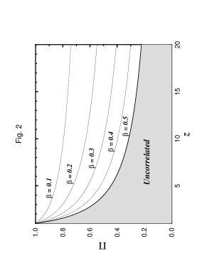
FIG. 2.: Phase diagram of the hierarchical-tree model. To each pair of values of $(\Pi,z)$ corresponds a value of $\beta$. We plot the iso-curves corresponding to several values of $\beta$. In the shaded area, marked “Uncorrelated,” the model predicts that $\beta=1/2$, i.e., that the units of the company are uncorrelated. Our empirical data suggests that most companies have values of $\Pi$ and $z$ in close to the curve for $\beta=0.2$.

Equation (19) is confirmed in the two limiting cases: when $\Pi=1$ (absolute control) $\beta=0$, while for all $\Pi<1/z^{1/2}$, decisions at the upper levels of management have no statistical effect on decisions made at lower levels, and $\beta=1/2$. Moreover, for a given value of $\beta<1/2$ the control level $\Pi$ will be a decreasing function of $z$: $\Pi=z^{-\beta}$, cf. Fig. 2. For example, if we choose the empirical value $\beta\approx 0.15$, then Eq. (19) predicts the plausible result $0.9\geq\Pi\geq 0.7$ for a range of $z$ in the interval $2\leq z\leq 10$.

IV Combining the Two Models

We started with two central empirical findings about firm growth rates. The model in Section II predicts one of those findings (the shape of the distribution) and the model in Section III predicts the other (the power law dependence of the standard deviation of output on firm size). This section addresses the relationship between the two models. First, we address concerns that the models might be contradictory and show that they are not. Then, we show how the models can be combined into a single model that predicts both of our empirical findings.

In the tree model, firm growth rates are potentially the result of many independent decisions. As a result, one might expect that the Central Limit Theorem would imply a Gaussian distribution of firm output. In fact, however, the distribution of outputs is not necessarily Gaussian.

To address the distribution of firm output in the tree model, it is necessary to make an assumption about the distribution from which each independent growth decision is drawn. No such assumption is needed to analyze the standard deviation of firm growth rates, but is needed to analyze the shape of the distribution.

In Fig. 3, we show the distribution of the inputs (i.e., of each independent decision) and the outputs for a tree with $z=2$, $\Pi=0.87$, and $n=10$. We find that for Gaussian distributed inputs, the output is not Gaussian in the tails. This finding is remarkable. First of all, with $z=2$ and $n=10$, the firm consists of 1024 units. With a probability to disobey of $1-0.87=0.13$, one would expect $0.13\times 1024\approx 133$ of the units to, on average, make independent decisions about their growth rates. Thus, even for non-Gaussian inputs, one can hypothesize that the output is close to Gaussian. Moreover, for Gaussian inputs, the sum of independent Gaussians is itself Gaussian. Thus, for every particular configuration of the disobeying links, the output distribution is Gaussian with variance $m\Delta$, which is a function of this random configuration. However, there are $2^{(z^{n+1}-z)/(z-1)}$ possible configurations of links each of which produce a Gaussian distribution with different integer $m$.

$$p_{n}(S_{1})=\sum_{m}p_{m}^{n}{1\over\sqrt{2\pi m\Delta}}e^{-(S_{1}-S_{0})^{2}/2m\Delta},$$ (20)

which is no longer Gaussian for the observed form of $p_{m}^{n}$.

FIG. 3.: Probability density for the output and input variables in the tree model. Here we have $z=2$, $\Pi=0.87$, and $n=10$. (a) Gaussian distribution of the input. (b) Exponential distribution of the input. (c) Data collapse of the output distribution for trees with different number of levels $n$. The other parameters remain unchanged and the input is exponentially distributed. It is visually apparent the similarity of the numerical results with the empirical data of Fig. 4(b) [4].

Figure 4 shows the probability $p_{m}^{n}$ to get a tree with given $m$ computed for all trees with a given number of levels $n$, $\Pi=0.87$, and $z=2$. As visually apparent in Fig. 4, this probability density is a non-trivial function, which is discussed in more detail in Appendix C. The final distribution of the firm output $S_{1}$ will be thus given by the convolution of two densities: $p_{m}^{n}$ and Gaussian with variance $m\Delta$

In a general case, it can be shown by martingale theory [15] that for any input distribution $f(x)$ with zero mean and finite variance $\Delta$, the output distribution converges for $n\to\infty$ to a distribution

$${1\over\sum_{1}(n)}g_{f}\left({x\over\sum_{1}(n)}\right),$$ (21)

where $g_{f}$ is a function that does not depend on $n$ but depends on $f$. Thus, we cannot expect to obtain a result that the output distribution must be exponential regardless of the input distribution. It would, however, be desirable to find some simple input distribution that yields the output distribution that we actually observe. Figure 3 also shows the output distribution when the input distribution is exponential in terms of $S_{1}-S_{0}$. For small $\sigma_{1}$, it practically coincides with Eq. (7). In this case, the output distribution is nearly exponential, and the slightly fatter wings that we observe are arguably consistent with our empirical results. Thus, in the limit of small $\sigma_{1}$, we can combine the models of the two sections by assuming that the dynamic process described in Sect. II provides the input distribution for the tree model in Sect. III. This additional assumption in the tree model then predicts both of our empirical findings. For large $\sigma_{1}$, the direct combination of two models needs additional fine-tuning.

FIG. 4.: Numerical estimation from exact enumeration of the coefficients $p_{n}^{m}$ of the generating function $p_{n}(s)$. It is visually apparent that the coefficients scale according to Eq. (B20) even for $n$ as small as 6. This result suggests that the companies have a self-similar structure.

V Conclusions

The two central results of our previous paper are that the distribution of company growth rates is exponential and the standard deviation of growth rates scales as a power law of firm size with scaling exponent $\beta\approx-0.2$. Any realistic theory of the firm in economics must be consistent with these empirical findings. In this paper, we have presented simple models that are consistent with our empirical findings. Indeed, the models have only two key assumptions. One is that each company has a natural size and the other is that decisions in hierarchical organizations are positively but imperfectly correlated. These models suggest that very simple mechanisms may provide insight into our empirical findings.

One limitation of the model in this paper is that it only predicts our results about one year growth rates. A complete model of the firm would also predict the distribution of growth rates over longer horizons. We believe that extending this model to additional periods would not provide a complete description of firm dynamics. In reality, the standard deviation of growth rates goes up as the time horizon increases. The attraction in our model to a stable company size prevents the distribution from spreading over time as much as we actually observe.

A Width of the Distribution of Final Sizes

The theory in Section III establishes results about the standard deviation of the growth rate. Our empirical results in the earlier paper concerned the standard deviation of the logarithmic growth rate defined as $\ln(S_{1}/S_{0})$. This appendix establishes the exact relationship between the standard deviation of the growth rate and the standard deviation of the logarithmic growth rate. Thus we will compute the width of the distribution of final sizes $S_{1}\equiv S_{0}\exp{r_{1}}$, that we designate by $\Sigma_{1}(S_{0})$. We can express $\Sigma_{1}$ as

$$\Sigma_{1}(S_{0})^{2}=\left\langle{S_{1}}^{2}\right\rangle-\left\langle{S_{1}}\right\rangle^{2}.$$ (A1)

Taking $\bar{r_{1}}(s_{0})\approx 0$, and assuming that the standard deviation of the distribution is small ($\sigma_{1}<1/\sqrt{2}$ which holds for companies with sales larger than $10^{6}$ dollars,) simple integrations lead to

$$\left\langle S_{1}\right\rangle=\int_{-\infty}^{+\infty}S_{1}~{}p(r_{1}|S_{0})~{}dr_{1}=\frac{S_{0}}{1-{\sigma_{1}}^{2}/2},$$ (A2)

and

$$\left\langle{S_{1}}^{2}\right\rangle=\int_{-\infty}^{+\infty}{S_{1}}^{2}~{}p(r_{1}|S_{0})~{}dr_{1}=\frac{{S_{0}}^{2}}{1-2{\sigma_{1}}^{2}}.$$ (A3)

Replacing these results onto (A1) and expanding in Taylor series, we obtain

$$\Sigma_{1}(S_{0})^{2} = {S_{0}}^{2}\left(1+2{\sigma_{1}}^{2}+4{\sigma_{1}}^{4}+\cdots-1-{\sigma_{1}}^{2}-3{\sigma_{1}}^{4}/4+\cdots\right)$$ (A4)

$$\approx (S_{0}\sigma_{1})^{2}(1+13{\sigma_{1}}^{2}/4).$$ (A5)

Thus, to first order, we obtain

$$\Sigma_{1}(S_{0})\sim{S_{0}}^{1-\beta}.$$ (A6)

B Analytical calculation of the variance of the growth rate for the hierarchical-tree model

This appendix provides a rigorous derivation of Eq. (16) Let, as before, $S_{1}$ represent the final size of a company with initial size $S_{0}$, and assume that the company has $n$ levels in its hierarchical tree. According to the rules of the model, the decision of the head of the company will only be followed by those units in the bottom level which are connected to the top by a chain of managers with “obeying links.” Thus, the number of units of the company that follow the policy of the head of the company $T_{n}$ can be related to the well known problem of the number of male descendents of a family after $n$ generations [13]. The solution is that for a $n$-level tree with $z$ branches the average number of units at the end is given by

$$\langle T_{n}\rangle=(z\Pi)^{n}.$$ (B1)

Now, let us look at the problem of calculating $\Sigma_{1}(S_{0})$. Our problem is slightly more complicated since it includes double averaging over all realizations of growth rates of independent units and over all possible configurations of the tree. Let us look at the $n^{\mbox{th}}$ level of a tree with a certain configuration of obeying and disobeying links. We can define clusters of units connected to one another through obeying links. Let us suppose that there are $M_{n}$ distinct clusters of size $\nu_{i}$. According to the rules of the model, all units in cluster $i$ share the same value of the annual change $\delta_{i}$. Thus, he final size of the company will be

$$S_{1}=S_{0}+\sum_{i=1}^{M_{n}}\nu_{i}\delta_{i},$$ (B2)

where $\delta_{i}$ are independent random variables with zero mean and variance $\Delta$.

The variance in $S_{1}$, for a given tree with $n$ levels, can be obtained by averaging over all realizations of $\delta_{i}$,

$$\Delta_{n}=\Delta\sum_{i=1}^{M_{n}}\nu_{i}^{2}\equiv m_{n}\Delta,$$ (B3)

where $m_{n}$ is a random variable depending solely on the structure of the tree

$$m_{n}=\sum_{i=1}^{M_{n}}\nu_{i}^{2}.$$ (B4)

To obtain ${\Sigma_{1}}^{2}$ we need now to average over all possible configurations of the hierarchical tree

$${\Sigma_{1}(n)}^{2}=\Delta\langle m_{n}\rangle.$$ (B5)

In order to calculate $\langle m_{n}\rangle$, we will start by computing the conditional average value $\left.\langle m_{n}\rangle\right|_{m_{n-1}}$, where $m_{n-1}$ refers to the previous level on the tree. A cluster of size $\nu_{i}$ in the $(n-1)$ level is connected to $z\nu_{i}$ units in the $n$-level; $\nu_{i}^{\prime}$ of the links are obeying, while $(z\nu_{i}-\nu_{i}^{\prime})$ are disobeying. The obeying links will give rise to a cluster of size $\nu_{i}^{\prime}$ in level $n$, while the disobeying links give rise to $(z\nu_{i}-\nu_{i}^{\prime})$ clusters of size one. Thus, we have

$$m_{n} = \sum_{i=1}^{M_{n-1}}\left({\nu_{i}^{\prime}}^{2}+(z\nu_{i}-\nu_{i}^{\prime})\right)$$ (B6)

$$= \sum_{i=1}^{M_{n-1}}({\nu_{i}^{\prime}}^{2}-\nu_{i}^{\prime})+z\sum_{i=1}^{M_{n-1}}\nu_{i}$$ (B7)

$$= \sum_{i=1}^{M_{n-1}}({\nu_{i}^{\prime}}^{2}-\nu_{i}^{\prime})+z^{n}.$$ (B8)

The probability of a configuration with a $\nu_{i}^{\prime}$ obeying links is

$${z\nu_{i}\choose\nu_{i}^{\prime}}\Pi^{\nu_{i}^{\prime}}(1-\Pi)^{z\nu_{i}-\nu_{i}^{\prime}}.$$ (B9)

By averaging over all possible configurations of links, we obtain

$$\langle m_{n}\rangle|_{m_{n-1}}=\sum_{i=1}^{M_{n-1}}\left\{\sum_{\nu_{i}^{\prime}=0}^{z\nu_{i}}{z\nu_{i}\choose\nu_{i}^{\prime}}\Pi^{\nu_{i}^{\prime}}(1-\Pi)^{z\nu_{i}-\nu_{i}^{\prime}}({\nu_{i}^{\prime}}^{2}-\nu_{i}^{\prime})\right\}+z^{n}.$$ (B10)

The series in (B10) can be calculated with one of the traditional “tricks.” Defining $q=1-\Pi$, $k=z\nu$, and $j=\nu_{i}^{\prime}$, we have

$$\sum_{j=0}^{k}{k\choose j}(j^{2}-j)\Pi^{j}(1-\Pi)^{k-j} = \Pi^{2}{\partial^{2}\over\partial\Pi^{2}}(\Pi+q)^{s}|_{\Pi+q=1}$$ (B11)

$$= k(k-1)\Pi^{2}.$$ (B12)

Replacing this result into (B10), we obtain

$$\langle m_{k}\rangle|_{m_{n-1}} = (z\Pi)^{2}\sum_{i=1}^{M_{n-1}}\nu_{i}^{2}-\Pi^{2}z\sum_{i=1}^{M_{n-1}}\nu_{i}+z^{n}$$ (B13)

$$= (z\Pi)^{2}m_{n-1}+(1-\Pi^{2})z^{n}.$$ (B14)

Hence $\langle m_{n}\rangle$ satisfies the recursion relation

$$\langle m_{n}\rangle=(z\Pi)^{2}\langle m_{n-1}\rangle+(1-\Pi^{2})z^{n},\qquad\quad\langle m_{0}\rangle=1.$$ (B15)

Writing the first few terms in the succession and induction show that

$$\langle m_{n}\rangle=(z\Pi)^{2}+(1-\Pi^{2})z^{n}\sum_{i=0}^{n-1}(z\Pi^{2})^{i}.$$ (B16)

Replacing the geometric series by its value and simple calculations lead to

$$\langle m_{n}\rangle=\left(z^{n}\frac{1-\Pi^{2}}{1-z\Pi^{2}}-(z\Pi)^{2n}\frac{(z-1)\Pi^{2}}{1-z\Pi^{2}}\right).$$ (B17)

Replacing this result into Eq. (B5), we get

$$\Sigma_{1}(n)^{2}=\Delta~{}\left(z^{n}\frac{1-\Pi^{2}}{1-z\Pi^{2}}-(z\Pi)^{2n}\frac{(z-1)\Pi^{2}}{1-z\Pi^{2}}\right).$$ (B18)

C Distribution of the output variable for the hierarchical-tree model

In this appendix we will derive the dependence of the variance of the distribution of growth rates for the hierarchical-tree model in a more formal way. At the same time we will get some insight onto the distribution of the number of end units that are connected by obeying links to the head of the tree. We will concentrate on the case in which the distribution of inputs is Gaussian.

Let us look at the the $n$-th level of the tree: We can define clusters of units which are connected to one another, in the tree, through obeying links. Thus, they share the same value of the annual size change. Supposing there are $M_{n}$ distinct clusters with sizes $\nu_{i}$, we have

$$N=z^{n}=\sum_{i=1}^{M_{n}}\nu_{i}.$$ (C1)

Since there is a set of possible tree structures for any given value of $\Pi$ (and $n$ and $z$), we should consider the set of all possible values of $M_{n}$ ($1\leq M_{n}\leq N$). Let us then denote the set of all partitions of $N$ into different clusters as $\Phi$, and each of these partitions as $\phi_{i}$. Naturally, the sum of the probabilities of each partition $P(\phi_{i})$ verifies

$$1=\sum_{\phi_{i}\epsilon\Phi}P(\phi_{i}).$$ (C2)

It is known that for large values of $N$, the number of different partitions behaves as $1/(\sqrt{48}N)~{}\exp{(\pi\sqrt{N/3})}$ [16].

Let us denote the probability density of the input variable $\delta$ as $f(\delta)$. The probability density for the output of a cluster of $s$ units connected by obeying links is

$$f(x=s\delta)=\frac{1}{s}~{}f\left(\frac{x}{s}\right).$$ (C3)

Thus, the distribution of the output variable $S=\sum_{j}^{M_{i}}x_{j}$ is given by

$$p_{n}(S)=\sum_{\phi_{i}\epsilon\Phi}\frac{1}{s_{1}}~{}f\left(\frac{x_{1}}{s_{1}}\right)~{}\ast~{}\frac{1}{s_{2}}~{}f\left(\frac{x_{2}}{s_{2}}\right)~{}\ast~{}...~{}\ast~{}\frac{1}{s_{M_{i}}}~{}f\left(\frac{x_{M_{i}}}{s_{M_{i}}}\right)P(\phi_{i}).$$ (C4)

where $g(y=x_{1}+x_{2})=f(x_{1})~{}\ast~{}f(x_{2})=\int f(x_{1})f(y-x_{1})dx_{1}$.

If $\delta$ is assumed to be Gaussian distributed with zero mean and unit variance:

$$f(\delta)=\frac{1}{\sqrt{2\pi}}\exp\left(-\frac{\delta^{2}}{2}\right),$$ (C5)

then the convolution leads to

$$g(x_{1}+x_{2}) = f(x_{1})~{}\ast~{}f(x_{2})$$ (C6)

$$= \frac{1}{\sqrt{2\pi(s_{1}^{2}+s_{2}^{2})}}~{}\exp\left(-\frac{y^{2}}{2(s_{1}^{2}+s_{2}^{2})}\right)$$ (C7)

$$= \frac{1}{\sqrt{s_{1}^{2}+s_{2}^{2}}}~{}f\left(\frac{y}{\sqrt{s_{1}^{2}+s_{2}^{2}}}\right).$$ (C8)

Replacing this result onto (C4), we obtain

$$p_{n}(S)=\sum_{\phi_{i}\epsilon\Phi}\frac{1}{\sqrt{\sum_{j=1}^{M_{i}}s_{i}^{2}}}~{}f\left(\frac{S^{2}}{\sqrt{\sum_{j=1}^{M_{i}}s_{i}^{2}}}\right).$$ (C9)

A simple analysis of Eq. (C9) shows that any two partitions, $\phi_{i}$ and $\phi_{k}$, are equivalent in terms of their output distributions if they verify

$$\sum_{j=1}^{M_{i}}s_{j}^{2}=\sum_{j=1}^{M_{k}}s_{j}^{2}=m.$$ (C10)

On the other hand, the triangular (or Schwarz) inequality allows us to determine the possible number of partitions that are not equivalent because of the constraints on the value of $s$

$$N=\sum_{j=1}^{N}1^{2}\leq\sum_{j=1}^{M_{i}}s_{i}^{2}\leq\left(\sum_{j=1}^{M_{i}}s_{i}\right)^{2}=N^{2}.$$ (C11)

Equations (C10-C11) imply that the sum in (C9) over different partitions can be replaced by a sum over $m$. Thus, we can write asymptotically

$$p_{n}(S)=\sum_{m=N}^{N^{2}}\frac{p_{m}^{n}}{\sqrt{m}}~{}f\left(\frac{S}{\sqrt{m}}\right),$$ (C12)

and, finally,

$$p_{n}(S)=\sum_{m=N}^{N^{2}}\frac{p_{m}^{n}}{\sqrt{2\pi m}}~{}e^{-S^{2}/2m},$$ (C13)

where $p_{m}^{n}$ is the total probability of all equivalent partitions with given $n$ and $m$.

The standard way to calculate the coefficients $p_{m}$ is to introduce a generating function [13]

$$p_{n}(S)=\sum_{m=N}^{N^{2}}p_{m}^{n}S^{m},$$ (C14)

which is a polynomial of order $N^{2}$. To obtain the recursion relations for $p_{n}(S)$, we need to distinguish the cluster of units which is connected to the top of the tree from those clusters that are not. For each level $n$ we have a matrix of coefficients $p_{\ell,k}$ that characterizes the probability of the partition with the cluster of $\ell$ elements connected to the head of the tree and the sum of squares of the rest of the cluster sizes equal to $k$. Thus, we can look at the tree as made of two parts, the one connected to the top, with size $\ell$, and the remaining of size $(N-\ell)$. Here we introduce the full generating function

$$p_{n}(y,S)=\sum_{\ell=0}^{N}~{}\sum_{k=N-\ell}^{(N-\ell)^{2}}p_{\ell,k}^{n}~{}y^{\ell}~{}S^{k},$$ (C15)

where $m={\ell}^{2}+k$.

The reduced generating function $p_{n}(S)$ can be obtained from the full generating function $p_{n}(y,S)$ if one formally puts $y^{\ell}=S^{\ell^{2}}$ in Eq. (C15). In order to obtain the recursion relation for the full generating function, let us consider a tree with $n+1$ levels as $z$ trees connected by another level of branches to the top. If a $n-$level tree is connected to the top by a disobeying link, which happens with probability $(1-\Pi)$, its clusters are totally independent of the other branches and we can use the reduced generating function $p_{n}(S)$. If, however, a $n-$level tree is connected to the top by a obeying link, which happens with probability $\Pi$, its clusters merge with the clusters of other such trees, and the full generating function $p_{n}(y,S)$ must be used. Thus, the generating function of level $n+1$ is related to the generating function of level $n$ through the recursion relation

$$p_{n+1}(y,S)=\left(\Pi p_{n}(y,S)+(1-\Pi)p_{n}(S)\right)^{z}.$$ (C16)

Unfortunately, to our knowledge, this recursion relation is too complex to allow any simplification or solution. Thus, we cannot obtain the distributions of cluster sizes for the different values of $n$. On the other hand, the problem of obtaining the average value of $\ell$ (which was earlier designated $\langle T_{n}\rangle$) and the variance $\Sigma_{1}(n)^{2}$ of the output variable is relatively simple [13]. Indeed

$$\langle T_{n}\rangle=\frac{\partial}{\partial y}p_{n}(y,S)|_{y=1,S=1}.$$ (C17)

Combining (C16) and (C17), we obtain

$$\langle T_{n+1}\rangle = \frac{\partial}{\partial y}p_{n+1}(y,S)|_{y=1,S=1}$$ (C18)

$$= z\Pi~{}\frac{\partial}{\partial y}p_{n}(y,S)|_{y=1,S=1}$$ (C19)

$$= z\Pi~{}\langle T_{n}\rangle.$$ (C20)

And we recover Eq. (B1). The variance can also be easily obtained as [13]

$$\langle m_{n}\rangle = \frac{\partial}{\partial S}p_{n}(S)|_{S=1}$$ (C21)

$$= \frac{\partial}{\partial y}y\frac{\partial}{\partial y}p_{n}(y,S)|_{y=1,S=1}+\frac{\partial}{\partial S}p_{n}(y,S)|_{y=1,S=1},$$ (C22)

which, after some algebra, leads to

$$\langle m_{n+1}\rangle=z\langle m_{n}\rangle+z(z-1)\Pi^{2}\langle T_{n}\rangle^{2},$$ (C23)

which is equivalent to Eq. (B15).

Although, as discussed earlier, the coefficients $p_{m}^{n}$ cannot be calculated analytically, we can use Eq. (C16) to find their values numerically (see Fig. 4). Moreover, for $z\Pi^{2}>1$ the coefficients $p_{m}^{n}$ of the reduced generating function $p_{n}(S)$ scale as

$$p_{m}^{n}={1\over(z\Pi)^{2n}}~{}g\left({m\over(z\Pi)^{2n}}\right)$$ (C24)

for large $n$. This can be proven applying the martingale theory [15]. Indeed, the sequence

$$\tilde{m}_{n}=\frac{m_{n}}{(z\Pi)^{2n}}+\frac{1-\Pi^{2}}{1-z\Pi^{2}}\left(1-\frac{1}{(z\Pi^{2})^{n}}\right)$$ (C25)

obeys the martingale conditions: From Eq. (B14) it follows that $\langle\tilde{m}_{n}\rangle|_{m_{n-1}}=\tilde{m}_{n-1}$. It also can be shown that $\tilde{m}_{n}$ has limited variance for any $n$, and hence it follows that for large $n$ the scaling relation (C24) is valid.

REFERENCES

- [1] B. B. Mandelbrot, J. Business 36, 394 (1963).
- [2] R. N. Mantegna and H. E. Stanley, Nature 376, 46–49 (1995); Nature 383, 587–588 (1996).
- [3] M. H. R. Stanley, L. A. N. Amaral, S. V. Buldyrev, S. Havlin, H. Leschhorn, P. Maass, M. A. Salinger, and H. E. Stanley, Nature 379, 804 (1996).
- [4] L. A. N. Amaral, S. V. Buldyrev, S. Havlin, H. Leschhorn, P. Maass, M. A. Salinger, H. E. Stanley, and M. H. R. Stanley, preceding article.
- [5] R. Gibrat, Les Inégalités Economiques (Sirey, Paris, 1931).
- [6] P. A. Samuelson and W. D. Nordhaus, Economics, 13th ed (McGraw-Hill, New York, 1989)
- [7] J. Leonard, National Bureau of Economic Research, working paper no. 1951, (1986).
- [8] M. Friedman, J. Economical Literature 30, 2129 (1992).
- [9] The reader may check that Eq. (5) is the right continuum limit of Eq. (4) by integrating Eq. (5) over time from to and by using that is a Gaussian random variable with zero mean and variance .
- [10] H. Risken, The Fokker-Planck Equation (Springer, Heidelberg, 1988).
- [11] R. Radner, Econometrica 61, 1109 (1993).
- [12] R. Lucas, Bell J. Economics 9, 508 (1978).
- [13] T. E. Harris, The Theory of Branching Processes (Prentice-Hall, Englewood Cliffs, 1963).
- [14] W. Li, Phys. Rev. A 43, 5240 (1991).
- [15] W. Feller, An Introduction to Probability Theory and Its Applications, Volume II, 2nd Edition (John Wiley and Sons, New York, 1971).
- [16] Handbook of Mathematical Functions, edited by M. Abramowitz and I. A. Stegun (National Bureau of Standards, Washington EC, 1964), p. 825.