Pseudo-Boundaries in Discontinuous 2-Dimensional Maps

Abstract

It is known that Kolmogorov-Arnold-Moser boundaries appear in sufficiently smooth 2-dimensional area-preserving maps. When such boundaries are destroyed, they become pseudo-boundaries. We show that pseudo-boundaries can also be found in discontinuous maps. The origin of these pseudo-boundaries are groups of chains of islands which separate parts of the phase space and need to be crossed in order to move between the different sub-spaces. Trajectories, however, do not easily cross these chains, but tend to propagate along them. This type of behavior is demonstrated using a “generalized” Fermi map.

The most obvious way to set particles into motion is to subject them to an external field. Yet, particle currents can be also induced by zero averaged time-dependent forces, provided an asymmetric potential is applied in the system. Recent studies of systems consisting of Brownian particles in periodic, locally asymmetric, potentials have shown that motion may be induced by periodic forcing, non-random noises or due to an oscillatory change in the potential profile [1]. Such rectification processes are interesting because they can lead to the generation of new microscopic pumping techniques. They may also provide some insight into the mechanism of protein motors [2]. Another example for a net directed motion of particles in periodic (both in time and space) potentials is found in a model describing the motion of a classical particle within an infinite set of equally spaced potential barriers, whose position and height oscillate periodically [3]. At each collision, the particle either crosses or reflects from the barrier, depending whether or not its kinetic energy is larger than the potential height. The special feature of this system (unlike these in Refs. [1]) is its chaotic deterministic nature. Chaotic dynamics are frequently studied by investigating the corresponding trajectories in the system’s phase space. Our system is one-dimensional with a time dependent Hamiltonian, hence it’s phase space is four-dimensional. The Poincarè method can be applied to reduce this 4-dimensional phase space into a 2-dimensional one by taking a surface lying in the phase space and studying the sets of intersections of different trajectories with this surface. Successive crossing points are computed using a 2-dimensional area-preserving map of the surface, the reduced phase space, onto itself. In order to inquire the features of this map, we constructed a picture of it’s 2-dimensional phase space by plotting the sets of points (which are the trajectories in the reduced phase space) starting at different initial conditions [4, 5].

In this paper we report and qualitatively explain an interesting phenomenon observed while studying this map. Pictures of the phase space, constructed for different values of the map’s parameters, displayed that the phase space consists of a stochastic sea, which a typical trajectory covers ergodically and some embedded islands, in which the motion is mainly regular over closed, elliptic-like, curves. This structure is quite common to many area-preserving maps. We did not observe Kolmogorov-Arnold-Moser (KAM) curves in our phase space. These curves of regular motion, if they exist, bound different parts of the stochastic sea, that is, prevent trajectories from leaving or entering them. According to the KAM theorem [6, 7, 8], KAM curves do not appear in discontinuous maps as is ours [9]. The origin of discontinuity in our map can be easily understood: Points in the phase space are divided into two classes each corresponding to either crossing or reflection from barriers. For each class the map is represented by one of its two possible “sub-maps”. Discontinuity appears on the boundaries between regions containing points of different classes (see Fig. 1).

Since KAM curves do not exist, the stochastic sea is a single connected unit with only a few islands excluded [10]. The motion over a connected (invariant) component of the phase space is ergodic and therefore a trajectory starting at almost any point in the stochastic sea, will eventually reveal this entire region. Numerical observations have shown that the number of iterations needed to explore completely the stochastic sea varies, within more than 3 orders of magnitude, for different values of the map’s parameters. In the cases when this number was considerably large, the stochastic sea seemed to be divided into smaller parts in which trajectories traveled for long time intervals before moving from the one to the other. The boundaries between the different parts are called pseudo (partial) boundaries. Their appearance does not violate the ergodicity hypothesis, it simply implies that it is valid only for time scales much larger than the characteristic escape time from each pseudo-bounded part of the stochastic sea.

Each KAM boundary is destroyed when the map’s control parameter exceeds some critical value. At the critical point an infinite number of gaps are formed in the torus and it turns into a Cantor set (hence called a cantorus) [11, 12]. As we continue to change the control parameter, the flux across the cantorus increases from its zero value at the critical point [13]. Thus, close to the critical point, the flux across a cantorus is low and cantorus serves as a pseudo-boundary. Cantori, like KAM tori, do not appear in discontinuous maps. We show in this paper that pseudo-boundaries are found in discontinuous maps due to other reasons. They are formed by chains of islands surrounding different areas of the phase space. In order to leave these areas, trajectories need to diffuse across the chains, which usually appear in groups. However, the motion in the vicinity of the chains, tends to be along the chains, in a way that resembles the regular motion over the chains.

In smooth maps, cantori and chains of islands are deeply related. For each torus, cantorus or chain of islands, there is a corresponding winding number (for definition of winding numbers see, for example, [14]). Tori and cantori have irrational winding numbers while chains of islands have rational ones. Green [15] has shown that close to any torus or cantorus, there are infinitely many chains of islands whose winding numbers are successive finite truncations of the continued fraction representing the irrational winding number of the torus or cantorus. It has also been shown [16, 17] that the flux across a cantorus is the limit of the flux across its approximating chains of islands. This last result means that chains of islands which approximate cantori that serve as pseudo-boundaries (i.e., which the flux across them is low) are pseudo-boundaries themselves. For discontinuous maps, in which winding numbers are meaningless, the properties of the chains should be studied differently, since they appear with no relation to cantori. A special emphasis should be given to the way in which trajectories behave when they are trapped between several adjacent chains.

We consider a classical particle of unit mass, moving within a one-dimensional sequence of equidistant potential barriers, each of an infinitesimal width and finite height, $H(t)$. The barriers oscillate with the same frequency and in phase. Their velocity is given by $v(t)=v_{b}g(t)$, while $H(t)=H_{0}[1+g(t)]$, where $g(t)=\sin(2\pi t)$. The particle moves freely between the barriers, occasionally colliding with them. At each impact it can either cross or be reflected from the barrier. It crosses the barrier if its kinetic energy in the reference frame of the barrier exceeds the height of the potential barrier at the moment of impact, i.e., $|V_{n}-v(t_{n})|>\sqrt{2H(t_{n})}$, where $t_{n}$ and $V_{n}$ are, respectively, the time of the $n$-th impact and the velocity of the particle before that impact. If the particle crosses the barrier, its velocity is not changed, i.e., $V_{n+1}=V_{n}$. If it is reflected, on the other hand, it acquires a new velocity: $V_{n+1}=-V_{n}+2v(t_{n})$. In order to calculate the moment of the next impact, one needs to consider the motion of both the particle and the barriers. We made the approximation that the distance traveled between two consecutive collisions is constant and equals to the distance between to barriers, $L$, as if the barriers do not change their position. We also assumed that in a case of reflection, the particle is reflected backward and therefore if $V_{n+1}$ has the same sign as $V_{n}$, we replace it with $-V_{n+1}$. A similar approach was used in Ref. [18] for the Fermi accelerator model (a ball bouncing between two walls [19]). Due to the periodicity of $g(t)$ only time modulo period (=1), which we denote as phase, is relevant, and two consecutive phases are related by $t_{n+1}=t_{n}+L\,/\,|V_{n+1}|\ \mbox{(mod 1)}$.

We chose the mean height of a barrier, $H_{0}$, to be the control parameter, while we set the other parameters $L=100$ and $v_{b}=\frac{1}{2}$. For the special case $H_{0}=\infty$, barrier crossing is impossible and the map reduces to the Fermi map [20]. For finite $H_{0}$, the map is discontinuous. Fig. 1 shows the discontinuity lines in the $(V-t)$ phase space which separate the regions mapped by the different sub-maps of crossing and reflection (for $H_{0}=500$). The map is area-preserving since both sub-maps are area-preserving and since their ranges do not overlap. For $V>V_{\rm max}\equiv 2\sqrt{H_{0}}+v_{b}$ and $V<V_{\rm min}\equiv-2\sqrt{H_{0}}+v_{b}$, points in the $(V-t)$ phase space are mapped only by the crossing sub-map (the kinetic energy is sufficiently large to cross the barriers at any phase), hence the motion in this part of the phase space is over the lines $V=V_{0}=\mbox{const}$. The stochastic sea lies between $V_{\rm min}$ and $V_{\rm max}$, including several islands. As already explained, a picture of it is made by starting at almost any one of its points, iterating the map a sufficiently large number of times and plotting the resulting trajectories, $\{(t_{n},V_{n});n=0,1,2\ldots\}$.

FIG. 1.: Regions in the $(t-V)$ phase space of points mapped by the sub-maps of crossing and reflection, for a barrier mean height $H_{0}=500$. The map is discontinuous over the curves separating between the different regions.

We performed this procedure for various values of $H_{0}$. For $H_{0}$ values below 1000, the stochastic sea was completely explored up to the resolution of the plots) after $10^{6}-10^{7}$ iterations. As expected, apart from some embedded chains of islands, the trajectory wandered in the entire region between $V_{\rm min}$ and $V_{\rm max}$. For $H_{0}>1000$, the situation was quite different. Fig. 2 depicts the velocities $V_{n}$ and phases $t_{n}$ of first $2\cdot 10^{10}$ collisions between the particle and the barriers. The velocities appear to remain smaller than 63, while the stochastic sea ranges between $V_{\rm min}=-99.5$ and $V_{\rm max}=100.5$.

A pseudo-boundary exists around $|V|\sim 63$. A closer look of that area of the phase space reveals a few adjacent chains of islands, located one above the other, whose shapes are similar to the boundary of the area plotted in Fig. 2. One of these chains is shown in Fig. 3. It is composed of two velocity branches, in the upper ($V>0$) and the lower ($V<0$) halves of the phase space, between which the motion alternates. The effect of this chain on the motion close to it is depicted in the inset of Fig. 3, showing an enlargement of a small segment of the chain. A narrow stochastic layer appears below the chain (above it, if the negative velocity branch is considered). We found that trajectories can move over this narrow layer for thousands of iterations before leaving it, usually falling back into the stochastic sea. Two features resemble the behavior close to a KAM torus or a cantorus: (1) the motion is restricted to one side of the boundary (the chain), and (2) the motion is correlated to the boundary and only gradually deviates from it. As for a cantorus, if the chain is long and narrow with only small gaps between the islands, there are only small areas from which a trajectory can jump from one of its sides to the other.

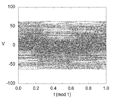
FIG. 2.: The subspace explored after $N=2\cdot 10^{10}$ iterations of the map for a barrier mean height $H_{0}=2500$. The points denote the velocity of the particle $V_{n}$ (y-axis), and the phase of the barrier, $t_{n}$ (x-axis), at the $n$-th ($n=1,2,\ldots,N$) collision.

Fig. 3 demonstrates the effect of a single long chain with islands located close to each other. The stochastic motion near such a chain is highly correlated. It, roughly, follows the regular motion over the chain and only slowly deviates from it. But when a pseudo-boundary appears, we usually observe a group of several chains, lying closely one above the other, and not only a single chain. Trajectories need to diffuse across all these chains in order to move to another sub-space. However, due to the character of the motion near the chains, they tend to move along them. Suppose a trajectory enters between a few chains, close to one of them. It propagates along the chain, while gradually moving away. If there are a few nearby chains, than while it moves away from one chain it gets closer to another, along which it propagates for subsequent iterations. This is an over-simplified picture since it is not always possible to relate the motion to a particular chain at each instance, yet, it qualitatively explains the character of the motion in this “band of chains”. The trajectory can be trapped between the chains for many iterations. If it succeeds in crossing all of them, it escapes. Usually, however, after spending some time wandering between the chains, it “falls back” into the stochastic sea. Fig. 4 depicts six chains and two stochastic trajectories. Note that while one of the trajectories (open squares) travels between the chains labeled 1 to 5, the other trajectory (dots) is restricted to the area above the chain labeled 5. Indeed, since the flux across this chain is very small, compared to the flux across the other chains (probably because of the fact that it consists of relatively many islands with small gaps between them), the chain labeled 5 (also shown in the inset of Fig. 3) serves as the natural limit for both sides of the pseudo-boundary.

FIG. 3.: A chain which appears in phase space around $|V|\sim 63$ for a barrier mean height $H_{0}=2500$. Its shape resembles the boundary of the area shown in Fig. 2. The inset is a magnification of a small part of the chain, showing few of its islands. A narrow stochastic layer is located just below the chain which serves as a pseudo-boundary. Trajectories that reaches the stochastic layer, may move over it for thousands of iterations before either falling back into the stochastic sea (the usual case) or crossing the chain (the rare scenario).

In conclusion, we have shown that long and narrow chains of islands may serve as pseudo-boundaries in discontinuous 2-dimensional maps. If a group of several adjacent chains surround a certain sub-space, they all need to be crossed in order to move to a different sub-space. However, in the vicinity of the chains, trajectories which stochastically wander between the islands tend to propagate along the chain, slowly moving from one chain to the other. Hence, the chains are not easily crossed and they form a pseudo-boundary.

Acknowledgments: The authors would like to thank to M. V. Jaric for useful discussions. This work was supported by the Sackler Institute for Solid State Physics at the Tel-Aviv University and by the Israel Science Foundation Grant No. 246/96-1.

FIG. 4.: A few adjacent chains of islands found in the phase space for a barrier mean height $H_{0}=2500$, forming together a pseudo-boundary. The numbers inside the islands label the different chains. The number of islands in the chains labeled 1 to 6, in the upper (lower) half of the phase space, are respectively: 27 (33), 37 (47), 49 (59), 60 (72), 420 (466), 157 (164). The dots and the open squares belong to two stochastic trajectories wandering, respectively, above and below the chain labeled 5. (Only a small part of the positive velocity branches of the chains is shown here.)

REFERENCES

- [1] M. O. Magnasco, Phys. Rev. Lett. 71, 1477 (1993); A. Ajdari, D. Mukamel, L. Peliti and J. Prost, J. Phys. 1 (France) 4, 1551 (1994); R. D. Astumian and M. Bier, Phys. Rev. Lett. 72, 1766 (1994); J. Prost, J. F. Chauwin, L. Peliti and A. Ajdari, Phys. Rev. Lett. 72, 2652 (1994); L. P. Faucheux, L. S. Bourdieu, P. D. Kaplan and A. J. Libchaber, Phys. Rev. Lett. 74, 1504 (1995).
- [2] Lodish Darnell, Molecular Cell Biology (W. H. Freeman, San Francisco, 1990).
- [3] M. V. Jaric and B. Sundaram, Bull. Am. Phys. Soc. 39, No. 1 , 538 (1994).
- [4] Y. Kantor and M. V. Jaric, (1996) (preprint).
- [5] O. Farago, M.Sc. Thesis, (1996).
- [6] A. N. Kolmogorov, Dokl. Akad. Nauk USSR 98, 527 (1954).
- [7] V. I. Arnold, Dokl. Akad. Nauk SSSR 138, 13 (1961) [Sov. Math. Dokl. 2, 501 (1961).]; Dokl. Akad. Nauk SSSR 142, 758 (1962) [Sov. Math. Dokl. 3, 136 (1962).]; Dokl. Akad. Nauk SSSR 145, 487 (1962).
- [8] J. Moser, On Invariant Curves of Area-Preserving Mappings on an Annulus., Nachr. Akad. Wiss. Gottingen, Math. Phys. K.1, p. 1 (1962).
- [9] For 2-dimensional nearly integrable maps, it appears that the continuity of the first derivative is a necessary condition for the existence of KAM curves, while the continuity of the second derivative is a sufficient one.
- [10] These elliptic curves are also KAM curves. In the area of phase space where they exist, the map is locally smooth.
- [11] S. Aubry, in Solitons and Condensed Matter Physics, edited by A. R. Bishop and T. Schneider (Springer, Berlin, 1978), p. 264.
- [12] I. C. Percival, in Nonlinear Dynamics and the Beam-Beam Interaction, edited by M. Month and J. C. Herrera, AIP Conf. Proc. No. 57 (AIP, New York, 1979), p. 302.
- [13] The flux across a curve is the fraction of trajectories (uniformly distributed on one of the curve’s sides) which cross the curve in a time unit (e.g. per iteration). This flux is proportional to the total area from which trajectories are mapped form one side of the curve to the other.
- [14] A. J. Lichtenberg and M. A. Lieberman, Regular and Stochastic Motion (Springer, New York, 1983).
- [15] J. Green, J. Math. Phys. 20, 1183 (1979).
- [16] R. S. MacKay, J. D. Meiss and I. C. Percival, Physica D 13, 55 (1984)
- [17] D. Bensimon and L.P. Kadanoff, Physica D 13, 82 (1984).
- [18] M. A. Lieberman and A. J. Lichtenberg, Phys. Rev. A 5, 1852 (1972).
- [19] E. Fermi, Phys. Rev. 75, 1169 (1949); S. Ulam, in Proceedings of the Fourth Berkeley Symposium on Mathematics, Statistics and Probability, Vol. 3, p. 315.
- [20] The standard Fermi map describes a ball bouncing between a fixed and an oscillating wall, while for our map describes a motion between two oscillating walls.