[

Nucleation, growth, and scaling in slow combustion

Abstract

We study the nucleation and growth of flame fronts in slow combustion. This is modeled by a set of reaction-diffusion equations for the temperature field, coupled to a background of reactants and augmented by a term describing random temperature fluctuations for ignition. We establish connections between this model and the classical theories of nucleation and growth of droplets from a metastable phase. Our results are in good argeement with theoretical predictions.

]

The kinetic process by which first-order phase transitions take place is an important subject of longstanding experimental and theoretical interest [1]. Nucleation is the most common of first-order transitions, and remains of a great deal of interest [2, 3, 4, 5, 6]. There are two fundamentally different cases, homogeneous and heterogeneous nucleation. Homogeneous nucleation is an intrinsic process where embryos of a stable phase emerge from a matrix of a metastable parent phase due to spontaneous thermodynamic fluctuations. Droplets larger than a critical size will grow while smaller ones decay back to the metastable phase [7, 8]. More commonplace in nature is the process of heterogeneous nucleation. There, impurities or inhomogeneities catalyze a transition by making growth energetically favorable.

Here we show that the concepts of nucleation and growth can be usefully applied to understand some aspects of slow combustion. We use a phase-field model of two coupled reaction-diffusion equations to study the nucleation and growth of combustion centers in two-dimensional systems. Such continuum reaction-diffusion equations have been used extensively in physics, chemistry, biology and engineering to describe a wide range of phenomena from pattern formation to combustion. However, the connection of reaction-diffusion equations to nucleation and interface growth has received little attention.

In a recent study of slow combustion in disordered media, Provatas et al. [9, 10] showed that flame fronts exhibit a percolation transition, consistent with mean field theory, and that the kinetic roughening of the reaction front in slow combustion is consistent with the Kardar-Parisi-Zhang (KPZ) [11] universality class. In this paper we make a further connection between slow combustion started by spontaneous fluctuations, and the classical theory of the nucleation and growth of droplets from a metastable phase.

We generalize the model of Provatas et al. by including an uncorrelated noise source $\eta({\bf x},t)$, as a function of position ${\bf x}$ and time $t$. The model then consists of equations of motion for the temperature field $T({\bf x},t)$ and the local concentration if reactants $C({\bf x},t)$. The temperature satisfies

$$\frac{\partial T({\bf x},t)}{\partial t}=D\nabla^{2}T-\Gamma[T-T_{0}]+R(T,C)+\eta.$$ (1)

The first term on the right-hand-side accounts for thermal diffusion, with diffusion constant $D$, the second term gives Newtonian cooling due to coupling with a heat bath of background temperature $T_{0}$, with rate constant $\Gamma$, and the third term $R(T,C)$ is the exothermic reaction rate as a function of temperature and concentration of reactants. The concentration satisfies

$$\frac{\partial C({\bf x},t)}{\partial t}=-\lambda_{1}R(T,C),$$ (2)

and the reaction rate obeys

$$R(T,C)=\lambda_{2}T^{3/2}e^{-A/T}C.$$ (3)

where $\lambda_{1,2}$ are constants, $A$ is the Arrhenius energy barrier, and Boltzmann’s constant has been set to unity. The noise is assumed to be uncorrelated and Gaussian of zero mean with a second moment $\langle\eta({\bf x},t)\eta({\bf x}^{\prime},t^{\prime})\rangle=2\epsilon\delta({\bf x}-{\bf x}^{\prime})\delta(t-t^{\prime})$, where the angular brackets denote an average, and $\epsilon$ is the intensity of the noise. Note that while the dynamics of the process is controlled by the activation term $e^{-A/T}$, the scale for energy is set by $T^{3/2}$. We choose the same values for the constants as those used in Ref. [10], which are approximately those for the combustion of wood in air: In physical units $D=1$ m²s^-1, $\Gamma=0.05$ s^-1, $T_{0}=0.1$ K, $A=500$ K, and the specific heat of wood, $c_{p}=5$ Jg^-1K^-1 (entering through $\lambda_{2}=8$). Length is measured in units of the reactant size, and time in units of those for the reaction to take place, $\lambda_{2}/\lambda_{1}$. The low background temperature is chosen to permit good numerical accuracy for systems of moderate size. The parameter $\epsilon$ was varied in the range $2\times 10^{-7}-11\times 10^{-7}$, and models the spontaneous fluctuations in heat in a random medium: $\epsilon=2\times 10^{-7}$ corresponds to slow, $\epsilon=5\times 10^{-7}$ to medium, and $\epsilon=11\times 10^{-7}$ to fast nucleation rate.

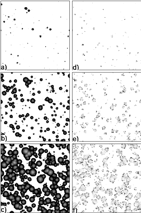
FIG. 1.: A snapshot of the process with medium nucleation rate, where $\epsilon=4.9\times 10^{-7}$. Gray scale images temperature, where black is the hottest region. The left column shows a system with uniform background ($c=1$) and the right column a case where $c=0.5$. In Fig. 1 a)-c) the time steps are $t=8$, $t=12$ and $t=16$, and in Fig. 1 d)-f) $t=10$, $t=15$ and $t=20$. The right panel features burning domains at significantly lower temperature, and with more ragged boundaries, due to the lower concentration of reactants.

We integrate these equations using Euler difference rules in space and time, with the smallest length $\Delta x=1$, and time $\Delta t=0.01$. Reactant units are randomly dispersed across the grid points with a probability $c$ so that $C({\bf x},t)=0$ for an unoccupied site and $C({\bf x},t)=1$ for an occupied site. Figure 1 shows typical results for a two-dimensional system of size $256\times 256$, with periodic boundary conditions. The gray scale images different temperatures, with black being the hottest regions. The left-hand panel shows the case for uniform concentration $c=1$, while the right-hand panel shows cooler and more ragged flame fronts that occur for $c=0.5$ (which is still well within the concentration for which the flame front can propagate, i.e. where $c\geq c^{*}$, and $c^{*}\approx 0.2$ for $\epsilon=0$).

The morphology of burnt and unburnt zones in these figures is strikingly similar to that for the nucleation and growth of crystallites from a supercooled melt [1], which is the motivation for our approach. We now briefly review the classical theories of nucleation and growth for such systems where a conservation law does not control the growth process.

The classical theory of nucleation was formulated in the 1930’s by Becker and Döring [7]. Their phenomenological theory has two main results: A description of the critical droplet, based on free energy considerations, and a rate equation for the growth of clusters. There exists also a modern theory [8], derived from first-principles, which generalizes the classical theory by, e.g., taking into account the finite interface thickness of the droplet domain walls. However, within the scope of this work, it is adequate to consider only the classical theory. In the classical theory, the extra free energy due to a droplet of stable phase, in a metastable background, is $\Delta F=-V\Delta f+A\sigma$, where $V$ is the volume of the droplet, $A$ is its area, $\sigma$ is surface tension, and $\Delta f$ is the difference in the bulk free energy densities between the metastable and stable phases. The critical radius $\rho^{*}$ of a droplet is obtained from through minimization: ${\partial\Delta F}/{\partial\rho^{*}}=0$. For circular droplets in two dimensions, this gives $\rho^{*}={\sigma}/{\Delta f}$ for the critical radius, and $\Delta F(\rho^{*})={\pi\sigma^{2}}/{\Delta f}$ for the height of the free energy barrier. For the metastable phase to decay, droplets with $\rho>\rho^{*}$ nucleate and grow; droplets smaller than the critical radius shrink and disappear. The rate-limiting process is the critical droplet, with energy barrier $\Delta F(\rho^{*})$, whose probability of occurrence is proportional to $\exp[-\Delta F(\rho^{*})/T]$.

After nucleation has occurred, the subsequent growth of droplets is often well described by the phenomenological Kolmogorov-Avrami-Mehl-Johnson (KAMJ) [12, 13, 14] model. This treatment describes many solid-solid and liquid-solid transformations, provided long-range interactions between droplets (which can be due to elastic effects, or diffusion fields) are of negligible importance. The KAMJ theory assumes that nucleation is a non-correlated random process with isotropic droplet growth occurring at constant velocity, where the critical radius is infinitesimal, and growth ceases when growing droplets impinge upon each other. As its basic result, the KAMJ description gives a functional form for the volume fraction of the transformed material:

$$X(t)=1-\exp[-\frac{V}{d+1}Iv^{d}(t-t_{0})^{d+1}]$$ (4)

for homogeneous nucleation, and

$$X(t)=1-\exp[-V\alpha v^{d}(t-t_{0})^{d}]$$ (5)

for heterogeneous nucleation. In the above, $v$ is the growth velocity, $I$ is the nucleation rate and $\alpha$ is the density of embryos with $\rho>\rho^{*}$ present in the beginning of the process. Homogeneous and heterogeneous nucleation are conveniently distinguished by the Avrami exponent, which is $d+1$, in Eq. (4), and $d$ in Eq. (5). The waiting time $t_{0}$ in Eqs. (4) and (5) accounts for initial transients.

In the KAMJ description there are two intrinsic length scales present in the system. The first one is the critical radius and the other is found by simple dimensional analysis. As seen from Eqs. (4) and (5), the process is characterized by two variables: the nucleation rate and the growth velocity. Using them, the characteristic length can be written as $\xi=(v/I)^{1/(d+1)}$ and the characteristic time scale as $\tau=(Iv^{d})^{-1/(d+1)}$. In practice, it is convenient to scale the time by the half-time of the transformation, $t_{1/2}$, since it is an easily accessible quantity both experimentally and computationally, and it can be used as a measure [5]. In the limit where $\xi\gg\rho^{*}$ there is only one length scale present [16]. During nucleation and growth this is the case up to the point when a connected cluster spans the system. As a consequence of this, scaling of $X(t)$ is expected, as we will show below.

The apparent simplicity of the KAMJ description is due to the fact that it incorporates no correlations. For cases where such correlations are minimal (as for the case considered herein), it has been quite successful in describing experimental data [3, 5], and theoretical generalizations can be readily made [2, 6, 15, 16]. The KAMJ description can be used in calculations of kinetic parameters and activation energies, and it provides information about the nature of the phase transition, i.e. if the process is diffusion or reaction (interface) controlled and if the process is influenced by inhomogeneities. Unfortunately, the basic KAMJ theory provides no information about the structural changes occurring during the phase transformation. Based on the same assumptions, Sekimoto [17] derived exact analytical expressions for two-phase correlation functions when $\xi\gg\rho^{*}$. Fourier transforming Sekimoto’s result for the two-point equal-time correlation function gives the structure factor:

$$S({\bf k},t)=\int d{\bf r}\mbox{~{}}[C_{2}({\bf x},t;{\bf x}+{\bf r},t)-C_{1}^{2}({\bf x},t)]e^{i{\bf k}\cdot{\bf r}},$$ (6)

where $C_{1}({\bf x},t)$ is the one-point correlation function equal to the KAMJ expression for transformed volume given in Eqs. (4) and (5). The two-point correlation function $C_{2}$ is

$$C_{2}({\bf x},t;{\bf x}+{\bf r},t)=C_{1}^{2}({\bf x},t)\exp[Iv^{2}\Psi(y)],$$ (7)

where

$$\Psi(y) = \frac{2}{3}\left[\arccos(y)-2y\sqrt{1-y^{2}}\right.$$ (9)

$$+y^{3}\left.\ln\left(\frac{1+\sqrt{1-y^{2}}}{y}\right)\right],$$

for $y\leq 1$, and $\Psi(y)=0$ for $y>1$. The variable $y$ is the normalized distance between two points. Combining Eqs. (6), (7), and (9) gives

$$S({\bf k},t) = 2\pi a^{2}e^{-\frac{2}{3}\pi Iv^{2}t^{\prime 3}}\times$$ (11)

$$\int_{0}^{1}dy\mbox{~{}}[e^{Iv^{2}t^{\prime 3}\Psi(y)}-1]yJ_{0}(aky),$$

where $J_{0}$ is the Bessel function of the zeroth kind, and $a=2vt^{\prime}$ with $t^{\prime}=t-t_{0}$.

We expect these theories to give a reasonable description of the growth of the flame fronts. In fact the agreement is much more impressive than we had anticipated. Of course, for combustion, the picture of nucleation and growth must be modified or re-interpreted in straightforward ways. For example, no shrinking of droplets, which herein correspond to burned patches, is possible. Also, instead of temperature in the Boltzmann probability weight, a quantity proportional to the intensity of noise sources $\epsilon$ must appear. Furthermore, the surface tension, evident in the fact that the burned patches are round, must have its origin in the dynamical description. Indeed, in the absence of nucleation it has been shown in Ref. [10] that the flame front roughens according to the KPZ interface equation, through which some of these correspondences can be made.

For example, the critical radius can be found as follows. We follow the method of Ref. [4, 18], and write the KPZ equation in circular coordinates as

$$\frac{\partial\rho}{\partial t}=\frac{D}{\rho^{2}}\frac{\partial^{2}\rho}{\partial\theta^{2}}-\frac{D}{\rho}+v\left(1+\frac{\rho^{2}_{\theta}}{2\rho^{2}}\right)+\frac{1}{\sqrt{\rho}}\mu(\theta,t),$$ (12)

where $\mu$ is a linear combination of an effective noise due to the random reactant, and the additive noise $\eta$. Next, we use the positive part of Eq. (46) in Ref. [10] with $v=(\Gamma\Lambda-\hat{\lambda}c)/\sigma$. The constants $\Lambda$, $\hat{\lambda}$ and $\sigma$ depend functionally on the temperature $T_{m}(x)$ that solves Eqs. (1) and (3) in the mean field limit. Their exact forms are given in Ref. [10]. Physically, the constant $\Lambda$ is proportional to the heat loss in the mean field limit, $\hat{\lambda}$ is proportional to the heat produced at the interface in the mean field limit, and $\sigma$ is analogous to surface tension. To find an expression for the critical radius, we apply perturbative analysis. Expanding $\rho$ and $\mu$ as $\rho(\theta,t)=\sum_{n}\rho_{n}(t)e^{in\theta}$, and $\mu(\theta,t)=\sum_{n}\mu(t)e^{in\theta}$, and substituting them into Eq. (12) together with the velocity gives $\rho^{*}=D\sigma/(\Gamma\Lambda-\hat{\lambda}c)$ for the the lowest order estimate for the critical radius of a radial flame front. When $\Gamma\Lambda\rightarrow\hat{\lambda}c$, $v\rightarrow 0$. In this limit the flame front does not propagate, since the heat lost to thermal dissipation exactly balances that due to thermal reaction, and the critical radius goes to infinity. Unfortunately, the numerical window in which the critical radius changes appreciably is narrow, and close to $c^{*}$. Hence, although our numerical work reported below is consistent with the above analysis, it does not permit a quantitative test of our estimate of $\rho^{*}$.

In our simulations we have typically used lattices of size $256\times 256$ with periodic boundary conditions, averaging over 1000 sets of initial conditions. Heterogeneous nucleation is modeled via inital fluctuations at $t=0$, and homogeneous nucleation as time dependent Gaussian fluctuations through $\eta$. First, we compare our results for the fraction of burnt reactant product $X(t)$ to the KAMJ theory. We have simulated systems with various noise intensities with uniform and disordered reactant concentrations to see the applicability of the KAMJ theory in relation to this model. In both uniform and disordered cases the simulations are in excellent agreement with the theory as seen in Fig. 2. The case of homogeneous nucleation fits the Avrami exponent $3$, while the heterogeneous case gives $2$, as expected. In the scaled plots we have discarded the waiting time $t_{0}$ (Eqs. (4) and (5)) since it is due to lattice effects and the fairly small system size, and therefore does not represent a true physical time scale.

FIG. 2.: Fraction burned vs. $t/t_{1/2}$ for various nucleation rates in homogeneous and heterogeneous nucleation in uniform and disordered systems. The inset shows the same data sets without scaling by $t_{1/2}$. The data is indistinguishable from the KAMJ theory (solid lines).

Next, we will focus on the structure factor in the case of uniform homogeneous nucleation, and compare $S({\bf k},t)$ for the temperature field from the simulations to Sekimoto’s theoretical prediction, Eq. (11), for various cases. Here, $S({\bf k},t)$ corresponds to correlations in reactant concentrations, i.e., between burnt zones. In the cases of both high and low noise, we find a quantitative agreement between the theory and simulations at late times, as seen Figs. 3 and 4. In order to use the theoretical prediction, Eq. (11), we measured the growth velocity of the radius of individual nucleation centers for various concentrations, and found it to be in agreement with previous results [9, 10], i.e. $R(t)\sim t$.

As seen from Figs. 3 and 4, the theoretical prediction underestimates the rate of phase transformation during

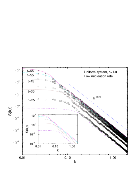
FIG. 3.: A plot of the structure factor vs. $k$ for various time steps at a low noise intensity (see Fig. 2) for a uniform system. The long-dashed line shows Porod’s law, which describes large-$k$ correlations of randomly-oriented interfaces of negligible width. In the inset we have replotted the theoretical curves to demonstrate the presence of wiggles more clearly.

the early stages, but is in good agreement at later times. This is because, for early times, contributions to the structure factor from the bulk interior of droplets, and from the diffuse surface width of droplets are comparable. For later times, the surface contributions (not considered in the KAMJ and Sekimoto theories) are negligible.

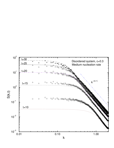
FIG. 4.: A plot of the structure factor vs. $k$ for various time steps at medium nucleation rate (see Fig. 2) for a disordered system. The dot-dashed line shows Porod’s law.

For a uniform background there are very pronounced wiggles present, as can be seen from Figs. 3 and 5. Their origin can be traced to the presence of the Bessel function in Eq. (11). The oscillations are due to the spherical shape of the burnt zones at early stages of the process

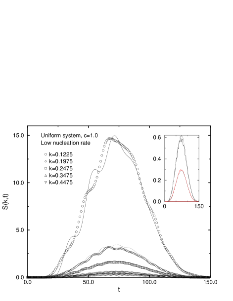
FIG. 5.: The structure factor vs. time for various $k$ at a low noise intensity for a uniform system. The symbols represent the data from the simulations and the lines display the theoretical prediction obtained by integrating Eq. (11). The inset shows the data for $k=0.3475$ and $k=0.4475$. The symbols display the data from the simulations, and the solid lines the theoretical prediction.

FIG. 6.: The structure factor vs. time for various $k$ at a medium nucleation rate for a disordered system. The symbols represent the data from the simulations and the lines display the theoretical prediction obtained by integrating Eq. (11).

when the growing regions have not yet merged with each other. That is, for early times, the structure factor is essentially the structure factor for a single droplet, with radius equal to the mean. The absence of wiggles in the case of quenched disorder, Fig. 4 and Fig. 6, is simply due to the fact that the disorder affects the spreading of the temperature field resulting in kinetic roughening. This is also clearly visible in Fig. 1. In Figs. 3 and  4 we have also compared the numerical results to Porod’s law, $S(k,t)\sim 1/k^{d+1}$ at large $k$ [1]. This should describe a locally flat and thin interface, and indeed we find excellent agreement for large $k$.

To confirm that the origin of the discrepancies between the theory and our simulations of the structure factor are due to the interface width, we also compared the results from the combustion model to a two-dimensional cellular automaton model with a nearest neighbor updating rule, using lattices of size $256\times 256$ and $1024\times 1024$. Using strictly nearest neighbor interactions for linear growth, so that there was no disorder in the front region, the CA model matched exactly the KAMJ result for the volume fraction (Eq. (4)), and Sekimoto’s result for the structure factor (Eq. (11)), as expected.

The constant growth velocity, and the scaling of $X(t)$ might suggest that the structure factor exhibits scaling, with the characteristic length increasing linearly in time, $L(t)\sim t$. However, as is evident from Figs. 3 and 4, this turns out not to be the case. This can also be seen from Eq. (11). At early times the structure factor follows approximately $\sim t^{5}$, and for late times it falls off exponentially. The reason is that the KAMJ theory applies to uncorrelated systems. The constant-velocity growth of a single domain is essentially due to the constant driving force of an excess chemical potential. But the distribution in sizes and in space of the droplets is due to their time and position of nucleation, implied by the nucleation rate. These two time scales are not proportional to each other, so no scaling results.

To conclude, we have studied the connection between the classical theory of nucleation and growth, and a model of slow combustion. We find that the reaction occurs with constant disorder dependent velocity with a linear scaling for the characteristic length $L(t)$ for the individual growing clusters. We have studied the structure factor of the temperature field and found good agreement with the theoretical predictions [17]. These results could be tested in a two-dimensional reaction-diffusion cell, or simply by slowly burning uncorrelated paper, i.e., with insignificant convection.

- [1] For a review see J. D. Gunton, M. San Miguel, and P. S. Sahni, in Phase Transitions and Critical Phenomena, edited by C. Domb and J. L. Lebowitz (Academic Press, London, 1983), Vol. 8.
- [2] V. Erukhimovitch, J. Baram, Phys. Rev. B 51, 6221 (1995).
- [3] N. Metoki, H. Suematsu, Y. Murakami, Y. Ohishi, Y. Fujii, Phys. Rev. Lett. 64, 657 (1990).
- [4] R. Kapral, R. Livi, G.-L. Oppo, A. Politi, Phys. Rev. E 49, 2009 (1994).
- [5] Y. Yamada, N. Hamaya, J.D. Axe, S.M. Shapiro, Phys. Rev. Lett. 53, 1665 (1984).
- [6] H.M. Duiker, P.D. Beale, Phys. Rev. B 41, 490 (1990).
- [7] R. Becker, W. Döring, Ann. Phys. (Leipzig) 24, 719 (1935). The classical nucleation theory is reviewed at length in F.F. Abraham, Homogeneous Nucleation Theory Academic Press, NY, 1974).
- [8] J. S. Langer, Ann. Phys. 54, 258 (1969).
- [9] N. Provatas, T. Ala-Nissila, L. Piché, M. Grant, Phys. Rev. E 51, 4232 (1995).
- [10] N. Provatas, T. Ala-Nissila, L. Piché, M. Grant, J. Stat. Phys. 81, 737 (1995).
- [11] M. Kardar, G. Parisi, and Y. C. Zhang, Phys. Rev. Lett. 56, 889 (1986).
- [12] A.N. Kolmogorov, Bull. Acad. Sci. USSR, Mat. Ser. 1, 335 (1937).
- [13] M. Avrami, J. Chem. Phys. 7, 1103 (1939).
- [14] W.A. Johnson, A. Mehl, Trans. Am. Inst. Min. Eng. 135 416, (1939).
- [15] R. M. Bradley, P. N. Strenski, Phys. Rev. B 40, 8967 (1989).
- [16] Y. Ishibashi, Y. Takagi, J. Phys. Soc. Jpn. 31, 506 (1971).
- [17] K. Sekimoto, Physica A 135, 328 (1986). The exponent of in front of the logarithmic term should be 3 instead of 2 in Eq. (3.14) of this paper.
- [18] It is also possible to derive the radial KPZ equation directly for the flame fronts: J. Hämäläinen, N. Provatas, T. Ala-Nissila, J. Timonen, unpublished (1996).
- [19] M. Karttunen and M. Grant, unpublished (1996).