Deviations from the Gaussian distribution of mesoscopic conductance fluctuations

Abstract

The conductance distribution of metallic mesoscopic systems is considered. The variance of this distribution describes the universal conductance fluctuations, yielding a Gaussian distribution of the conductance. We calculate diagrammatically the third cumulant of this distribution, the leading deviation from the Gaussian. We confirm random matrix theory calculations that the leading contribution in quasi-one dimension vanishes. However, in quasi two dimensions the third cumulant is negative, whereas in three dimensions it is positive.

I Introduction

About ten years ago the universal conductance fluctuations (UCF) were discovered in mesoscopic, metallic samples[1, 2, 3]. The electronic conductance of these samples shows reproducible sample to sample fluctuations. The fluctuations are called universal because their magnitude is independent of the sample parameters such as the mean free path $\ell$, and the average conductance $\langle g\rangle$. The dependence on sample dimension is weak. Studies have mainly focused on the variance of the fluctuations, which is the leading and the universal part of the fluctuations.

The conductance being a random variable showing such large fluctuations, one realized that one should consider its full distribution. It was soon clear that the first higher cumulants of the conductance are proportional to [4]

$$\langle g^{n}\rangle_{c}\propto\langle g\rangle^{2-n},\qquad n<g_{0},\;\langle g\rangle\gg 1.$$ (1)

Here the conductance is measured in units of $e^{2}/\hbar$, $g_{0}$ is the mean conductance at the scale $\ell$, $\langle\ldots\rangle$ denotes the ensemble averaging, and the subscript $c$ indicates cumulants. In the metallic regime far from localization, where $\langle g\rangle\gg 1$, the higher cumulants are thus small, and the distribution of the conductance is therefore roughly Gaussian. However, for $n\gtrsim g_{0}$ the decrease in magnitude of cumulants as described by Eq. (1) is changed into a very rapid increase ($\propto\exp[g_{0}^{-1}n^{2}]$). This leads to the log-normal tails of the distribution [4]. With increasing disorder, the log-normal tails become more important. Although the calculation of the full conductance distribution on the threshold of localization ($\langle g\rangle\sim 1$) is today out of reach, it is quite plausible that the whole distribution crosses over to a log-normal shape in the strongly localized regime (see Refs. [5] and [6] for a discussion). Indeed, it is well known that in the strongly localized regime in one dimension the conductance is given by the product of transmission amplitudes, yielding a log-normal distribution [7, 8, 9, 10].

Although high order cumulants govern the tails of the distribution, they do not affect it near the center. A deviation from the Gaussian distribution near the center should be revealed, first of all, in the lowest nontrivial cumulants. An important step in this direction was the recent calculation of the third cumulant of the distribution using random matrix theory by Macedo [11]. He found for the orthogonal ($\beta=1$) and symplectic ensemble ($\beta=4$) that the third cumulant of the conductance is proportional to $1/g^{2}$, thus the leading term given by Eq. (1) vanishes (see for instance Ref. [12] for the definitions of the ensembles). For the unitary ensemble ($\beta=2$) even this sub-leading term vanishes. The physical reason behind this is not clear. (We recently learned that the same result in quasi one dimension was found by Tartakovski [13] by the scaling method described in Ref. [14].) However, random matrix theory is only valid in quasi one dimensional systems. Therefore, it was not known whether this cancelation is unique to one dimension, or holds also in higher dimensions, which might indicate an overlooked symmetry of the system. That such a possibility exists was also suggested by the fact that the leading-order contribution to the third cumulant of the density of states vanishes in two dimensions [4]. The question whether or not the cancelation holds in two and three dimensions was a major motivation for this work.

Let us finally mention that related to the conductance distribution, recently third cumulants [15] and the full distribution functions [16] of two related transmission quantities were calculated. These quantities, the speckle transmission and the total transmission, were measured in scattering experiments with electro-magnetic waves (light and microwaves) [17, 18]. In the regime considered, these distributions are independent of dimension. On a diagrammatic level this can be understood: The diagrams for the cumulants of the speckle and the total transmission are loop-less diagrams [16]. The diagrams for the cumulants of the conductance, however, contain loops, and will therefore be, a priori, dimension dependent. For the electro-magnetic waves the Landauer approach was used, however, for conductance properties this yields the same results as the Kubo approach [19, 20]. Therefore, the calculations presented below are also valid for classical waves.

In the present paper we will calculate the third cumulant of the conductance for any rectangular geometry in the metallic regime in quasi one, quasi two, and three dimensions. In section II we review the formalism for calculating conductance fluctuations. In section III it is described how the leading diagrams can be found. In section III A we calculate the third cumulant and discuss its dimension dependence. After considering the effects of inelastic scattering, we end with a conclusion.

II Conductance fluctuations

In this section we introduce our diagrammatic approach, to a large extent following the detailed paper of Lee, Stone, and Fukuyama [21]. We consider a sample with a rectangular geometry with sizes $L_{x}\times L_{y}\times L_{z}$; the conductance is measured across the z-direction. The scatterers are isotropic point scatterers. The scattering is calculated in second order Born approximation, which assumes weak scattering. (The present calculation can be easily extended beyond second order Born, this will yield the same results provided the correct mean free path is taken [22, 23].) We consider the metallic, mesoscopic regime, which is characterized by the inequalities $1/k\ll\ell\ll L_{z}$, where $k$ denotes the Fermi wavenumber; $\ell$ is the mean free path, related to the scatterer density $n$ and scatterer strength $v$ as $\ell=4\pi/n|v|^{2}$. The relaxation time is given by $\tau=\ell/(2k)$. Incoherent scattering is first neglected, that is, the incoherence length is much larger than any system size, $L_{\rm in}\gg L_{x},L_{y},L_{z}$.

The conductance and its cumulants are calculated with the Kubo formula. The transport through the sample is given by the so called ladder diagrams or diffusons, describing the multiple scattering of the electrons on the scatterers. In the conductance diagram the field creates an electron-hole pair at a current vertex somewhere in the sample, after some diffuse propagation this pair annihilates. This diagram thus contains a bubble, the corresponding propagator ${\cal L}$ obeys the diffusion equation:

$$-\nabla^{2}_{1}{\cal L}({\bf r}_{1},{\bf r}_{2})=\frac{1}{2\pi\nu\tau^{2}D}\delta({\bf r}_{1}-{\bf r}_{2}),$$ (2)

where $D$ is the diffusion constant. (Correspondence with units often used with classical waves is found by identifying: $\hbar=1$, $m=1/2$, $\nu=k/(4\pi^{2})$, $D=2k\ell/3$.)

As mentioned we restrict ourselves to the conductance in the z-direction. The current is restricted to the z-direction by imposing fully reflecting boundaries in the $x$ and $y$ direction, and fully conducting boundaries in the $z$-direction:

$${\cal L}({\bf r}_{1},{\bf r}_{2})|_{z_{1}=0,z_{1}=L_{z}}=0\,,\qquad\frac{\partial{\cal L}({\bf r}_{1},{\bf r}_{2})}{\partial x_{1}}|_{x_{1}=0,x_{1}=L_{x}}=\frac{\partial{\cal L}({\bf r}_{1},{\bf r}_{2})}{\partial y_{1}}|_{y_{1}=0,y_{1}=L_{y}}=0,$$ (3)

and similarly for the ${\bf r}_{2}$ dependence. For rectangular geometries it is useful to write the solution of the diffuson propagator in (discrete) momentum space. Following Ref.[21] (in present work there is an extra factor $1/(2\pi\nu\tau)$ in the diffuson), we write the diffuson as

$${\cal L}({\bf r}_{1},{\bf r}_{2})=\frac{1}{2\pi\nu\tau^{2}D}\sum_{i_{z}=1}^{\infty}\sum_{i_{x}=0}^{\infty}\sum_{i_{y}=0}^{\infty}\frac{Q_{i}({\bf r}_{1})Q_{i}({\bf r}_{2})}{\lambda_{i}}$$ (4)

where $i$ is the momentum vector $(i_{x},i_{y},i_{z})$. The $Q_{i}$’s are the normalized, orthogonal eigenfunctions

$$Q_{i}({\bf r})=\sqrt{\frac{2}{L_{x}}\frac{2}{L_{y}}\frac{2}{L_{z}}}\,\sin\left(\frac{\pi zi_{z}}{L_{z}}\right)\cos\left(\frac{\pi xi_{x}}{L_{x}}\right)\cos\left(\frac{\pi yi_{y}}{L_{y}}\right).$$ (5)

Note that these eigenfunctions are not properly normalized if $i_{x}=0$ or $i_{y}=0$, in which case one has to replace $\cos\left(\frac{\pi xi_{x}}{L_{x}}\right)$ or $\cos\left(\frac{\pi yi_{y}}{L_{y}}\right)$ by $1/\sqrt{2}$. The eigenvalues $\lambda_{i}$ in Eq.(4) are

$$\lambda_{i}=\frac{\pi^{2}}{L_{z}^{2}}\left[i_{z}^{2}+i_{x}^{2}\left(\frac{L_{z}}{L_{x}}\right)^{2}+i_{y}^{2}\left(\frac{L_{z}}{L_{y}}\right)^{2}\right]$$ (6)

The longitudinal momentum $i_{z}$ takes positive integer values; the transverse momenta $i_{x}$ and $i_{y}$ can in addition also be zero. In quasi two dimensional (2D) geometries one has $L_{x}\ll L_{z}$ and only the terms with $i_{x}=0$ contribute in the eigenvalues. In quasi one dimensional (1D) samples also $L_{y}\ll L_{z}$, and $i_{y}$ is essentially restricted to zero. On the other hand, for very wide geometries $i_{x}^{2}\left(L_{z}/{L_{x}}\right)^{2}$ becomes a continuous variable and the sum over the $x$-variable (or $y$-variable) becomes an integral. The average value of the dimension-less conductance $\langle g\rangle$ is

$$\langle g\rangle=2\pi\nu D\frac{L_{x}L_{y}}{L_{z}}.$$ (7)

The inverse of this, $1/\langle g\rangle$, will be a small parameter in our diagrammatic expansion.

A Hikami-boxes

For the calculation of the second and higher order cumulants of $g$, we need the vertices describing the interference between two diffusons. These vertices are known as Hikami-boxes[24, 25]. Formally they arise from the spatial derivatives $\partial/\partial{\bf r}_{\alpha}$ and $\partial/\partial{\bf r^{\prime}}_{\beta}$ in the Kubo formula for $\sigma_{\alpha,\beta}({\bf r},{\bf r^{\prime}})$, where the indices $\alpha,\beta=x,y,z$ label the directions of the incoming and outgoing current. We have drawn the boxes in Fig. 1, the corresponding expressions are labeled $H_{a}$ to $H_{f}$, respectively:

$$H_{a} = 4\pi\nu\tau^{3}\frac{\delta_{\alpha,\beta}}{3},$$ (9)

$$H_{b} = 2\pi\nu\tau^{3}\frac{\delta_{\alpha,\beta}}{3},$$ (10)

$$H_{c1} = 4\pi i\nu\tau^{4}{\bf q}^{\alpha}_{2}\frac{k}{3},$$ (11)

$$H_{c2} = -H_{c1},$$ (12)

$$H_{d} = 2\pi\nu\tau^{4}D\left[-2{\bf q}_{1}\cdot{\bf q}_{3}-2{\bf q}_{2}\cdot{\bf q}_{4}-({\bf q}_{1}+{\bf q}_{3})\cdot({\bf q}_{2}+{\bf q}_{4})\right],$$ (13)

$$H_{e} = 4\pi\nu\tau^{3}\frac{\delta_{\alpha,\beta}}{3},$$ (14)

$$H_{f} = -2\pi\nu\tau^{5}\frac{\delta_{\alpha,\beta}}{3}.$$ (15)

The ${\bf q}$’s are the momenta of the diffusons (the wavy lines), as numbered according Fig. 1. As the conductance is calculated in the z-direction, $\alpha$ and $\beta$ are taken $z$. Likewise, only the z-component of the momentum in $H_{c}$ will be taken into account. $H_{c}$ comes in two flavors: $H_{c1}$ and $H_{c2}$. $H_{c2}$ has an additional minus sign due to the reversed orientation of the advanced and retarded propagators of the current vertex. We used that the diffusons vary slowly on length scales of the mean free path, i.e. $q\ell\ll 1$. Finally, other boxes are sub-leading.

B UCF calculation

For clarity we briefly present the UCF calculation using this formalism. The UCF-diagrams are connected diagrams containing two conductivity bubbles and thus four current vertices. Its diagrams are shown in Fig. 2. The UCF diagrams contain two four-boxes ($H_{a}$ or $H_{b}$) and two diffusons. For the orthogonal ensemble the combinatorial factor for the upper diagram is 4. The lower diagram has combinatorial factor 2, and the two Hikami vertices bring, comparing Eq. (9) to Eq. (10), an additional factor of $2^{2}$. Thus one finds a pre-factor 12 for the sum of all diagrams with respect to a single diagram of the upper topology. (In the unitary ensemble cooperons do not contribute and this would be a factor 6.) For each incoming or outgoing current vertex there is a factor $2k/L_{z}$. It arises from the expression $1/(mL_{z})\to 2/L_{z}$, that can be read off from Eq.(2.5) in Ref. [21], and the wavenumber $k$ that originates from each derivative in the Kubo formula. Next, we use the Fourier decomposition of the diffusons Eq.(4) and interchange the sum over the eigenvalues with the spatial integrals. The two diffusons interfering at the Hikami-box yield the orthogonality relations: $\int d{\bf r}Q_{i}({\bf r})Q_{j}({\bf r})=\delta^{(3)}_{i,j}$. One finds

$$\langle g^{2}\rangle_{c} = 12\left(\frac{2k}{L_{z}}\right)^{4}\left(\frac{1}{2\pi\nu\tau^{2}D}\right)^{2}\left(\frac{2\pi\nu\tau^{3}}{3}\right)^{2}\int d{\bf r}_{1}\int d{\bf r}_{2}{\cal L}({\bf r}_{1},{\bf r}_{2})^{2}$$ (16)

$$= \frac{12}{L_{z}^{4}}\sum_{i,j}\frac{1}{\lambda_{i}\lambda_{j}}\int d{\bf r}_{1}Q_{i}({\bf r}_{1})Q_{j}({\bf r}_{1})\int d{\bf r}_{2}Q_{i}({\bf r}_{2})Q_{j}({\bf r}_{2})$$ (17)

$$= \frac{12}{L_{z}^{4}}\sum_{i,j}\frac{1}{\lambda_{i}\lambda_{j}}(\delta_{i_{z},j_{z}}\delta_{i_{x},j_{x}}\delta_{i_{y},j_{y}})^{2}$$ (18)

$$= \frac{12}{\pi^{4}}\sum_{i_{z}=1,i_{x}=0,i_{y}=0}^{\infty}\left(i_{z}^{2}+i_{x}\frac{L_{z}^{2}}{L_{x}^{2}}+i_{y}\frac{L_{z}^{2}}{L_{y}^{2}}\right)^{-4}.$$ (19)

In quasi one dimension this yields $\frac{12}{\pi^{4}}\sum_{i_{z}=1}^{\infty}i_{z}^{-4}=\frac{2}{15}$, which is the well-known result for the UCF in quasi one dimension[21].

III The third cumulant

We now study the third cumulant. First, we rewrite Eq.(1) into a relation for the relative cumulants: $\frac{\langle g^{n}\rangle_{c}}{\langle g\rangle^{n}}\propto\langle g\rangle^{2-2n}$. The inverse power of $\langle g\rangle$ on the right hand side can be interpreted as the number of Hikami four-boxes in the diagrams. Thus the third cumulant diagram contains four Hikami four-boxes. Indeed, it proves impossible to create $\langle g^{3}\rangle_{c}$ diagrams with less boxes. Diagrams with more boxes are sub-leading as they are of higher power of $1/\langle g\rangle$, which is a small parameter. In diagrammatic approaches it is often tricky to find all the relevant diagrams; already for the much simpler set of UCF diagrams there was considerable discussion in the literature. We used the following considerations to find the set of diagrams for the third cumulant: The diagrams have six current vertices: three incoming ones and three outgoing ones. The diagrams contain four 4-point vertices and each vertex has at least two diffusons attached to it, see Fig. 1. This leaves two possibilities: there are three boxes with each two diffusons and one box with four diffusons; or, are two boxes with two diffusons and two boxes with three diffusons each. It is now an easy exercise to see that there are only four possible basic topologies. They are drawn in Fig. 3. The dots represent the 4-point vertices; the lines represent diffusons. The next step is to insert the Hikami-boxes and connect them in all possible ways to the diffusons. This yields many diagrams, yet not in all diagrams the outgoing electron-hole pair is the same as the incoming electron-hole pairing. Such diagrams are not the product of three conductance bubbles; they do not contribute to the $\langle g^{3}\rangle_{c}$ process and are left out. We end up with the diagrams represented in Fig. 4. In the figure there are also diagrams of the same order with one six-box and two four-boxes. They can be obtained by contracting one diffuson in the diagrams with four-boxes. In physical terms the six-box diagrams correspond to processes where after an interference process, the amplitudes do not combine into a diffuson. Instead, the amplitudes interact again directly without being scattered.

A Evaluation of the diagrams

We calculate the diagrams for quasi-1D, quasi-2D, and 3D geometries. The calculation goes similar to the UCF-calculation, that is, the sums over the momenta are taken outside the spatial integrals. If two internal diffusons interfere, the spatial integrals bring the orthogonality relations as used for the UCF calculation. However, two complications arise. First, at the Hikami vertices not only two, also three, or four diffusons interfere (as is seen from from the Figs. 3 and 4), this gives more complicated structures. Secondly, Hikami-boxes $H_{c}$ and $H_{d}$ are $q$-dependent, corresponding to spatial derivatives of the diffusons. We therefore introduce the matrices $R$, $S$, and $T$, which describe the interaction of the diffusons at the vertices.

In the diagrams e.i), e.ii), e.v), and e.vi) of Fig. 4 four diffusons, two with momentum $i$, and two with momentum $j$ interfere. The x-components of the diffusons couple as

$$R_{i_{x},j_{x}}=\left(\frac{2}{L_{x}}\right)^{2}\int_{0}^{L_{x}}dx\cos^{2}\left(\frac{i_{x}x\pi}{L_{x}}\right)\cos^{2}\left(\frac{j_{x}x\pi}{L_{x}}\right)=\frac{1}{L_{x}}\left[1+\frac{1}{2}(1-\delta_{i_{x},0})\delta_{i_{x},j_{x}}\right]$$ (20)

The y-components yield exactly the same integral, see Eq.(5), and also the z-components yield the same expression. These diagrams will thus be proportional to $R_{i_{z},j_{z}}R_{i_{x},j_{x}}R_{i_{y},j_{y}}$.

In most other diagrams three diffusons interfere at a Hikami box $H_{c1}$, this box brings a derivative $\partial/\partial_{z}$. The matrix $S$ describes the effect of this derivative on the z-component, the $T$ describes the integrals over x and y components.

$$S_{i_{z},j_{z},k_{z}} = \left(\frac{2}{L_{z}}\right)^{3/2}\int_{0}^{L_{z}}dz\left(\frac{i_{z}\pi}{L_{z}}\right)\cos\left(\frac{i_{z}z\pi}{L_{z}}\right)\sin\left(\frac{j_{z}z\pi}{L_{z}}\right)\sin\left(\frac{k_{z}z\pi}{L_{z}}\right)$$ (21)

$$= \frac{i_{z}\pi}{L_{z}\sqrt{2L_{z}}}(-\delta_{i_{z},j_{z}+k_{z}}+\delta_{j_{z},i_{z}+k_{z}}+\delta_{k_{z},i_{z}+j_{z}})$$ (22)

$$T_{i_{x},j_{x},k_{x}} = \left(\frac{2}{L_{x}}\right)^{3/2}\int_{0}^{L_{x}}dx\cos\left(\frac{i_{z}z\pi}{L_{z}}\right)\cos\left(\frac{j_{z}z\pi}{L_{z}}\right)\cos\left(\frac{k_{z}z\pi}{L_{z}}\right)$$ (23)

$$= \frac{1}{\sqrt{L_{x}}}(\delta_{i_{x},0}\delta_{j_{x},k_{x}}\!+\!\delta_{j_{x},0}\delta_{i_{x},k_{x}}\!+\!\delta_{k_{x},0}\delta_{i_{x},j_{x}}\!-\!2\delta_{i_{x},0}\delta_{j_{x},0}\delta_{k_{x},0})\quad\mbox{(if $i_{x}$, $j_{x}$, or $k_{x}=0$)}$$ (24)

$$= \frac{1}{\sqrt{2L_{x}}}(\delta_{i_{x},j_{x}+k_{x}}+\delta_{j_{x},i_{x}+k_{x}}+\delta_{k_{x},i_{x}+j_{x}})\qquad\qquad\mbox{(else)}$$ (25)

The box $H_{c2}$ has a minus sign resulting in $-S_{i_{z},j_{z},k_{z}}T_{i_{x},j_{x},k_{x}}T_{i_{y},j_{y},k_{y}}$.

The diagrams can now be written in terms of the $R,S,T$. The pre-factors, the combinatorial factors, and the sum over the momenta are included. The third cumulant is given by the sum of diagrams $\langle g^{3}\rangle_{c}=\sum F$, where the $F$’s are,

$$F_{a.i}+F_{a.ii} = -144r\sum_{i,j,k}\frac{1}{\lambda_{i}^{3}\lambda_{j}\lambda_{k}}\,S_{i_{z},j_{z},k_{z}}^{2}T_{i_{x},j_{x},k_{x}}^{2}T_{i_{y},j_{y},k_{y}}^{2}$$ (27)

$$F_{b.i}+F_{b.ii}+F_{e.iii}+F_{e.iv} = 72r\sum_{i,j}\frac{1}{\lambda_{i}^{3}\lambda_{j}^{2}}\,\left[\frac{\pi^{2}}{L_{z}^{3}}\left(\frac{3}{2}i_{z}^{2}\delta_{i_{z},j_{z}}\!+\!i_{z}^{2}\right)R_{i_{x},j_{x}}R_{i_{y},j_{y}}\right.$$ (29)

$$\left.+\frac{\pi^{2}}{L_{x}^{3}}\left(\frac{3}{2}i_{x}^{2}\delta_{i_{x},j_{x}}\!+\!i_{x}^{2}\right)R_{i_{z},j_{z}}R_{i_{y},j_{y}}+\frac{\pi^{2}}{L_{y}^{3}}\left(\frac{3}{2}i_{y}^{2}\delta_{i_{y},j_{y}}\!+\!i_{y}^{2}\right)R_{i_{x},j_{x}}R_{i_{z},j_{z}}\right]$$

$$F_{c.i} = -48r\sum_{i,j,k}\frac{1}{\lambda_{i}^{2}\lambda_{j}^{2}\lambda_{k}}\,S_{i_{z},j_{z},k_{z}}^{2}T_{i_{x},j_{x},k_{x}}^{2}T_{i_{y},j_{y},k_{y}}^{2}$$ (30)

$$F_{c.ii}+F_{c.iii} = -120r\sum_{i,j,k}\frac{1}{\lambda_{i}^{2}\lambda_{j}^{2}\lambda_{k}}\,S_{k_{z},i_{z},j_{z}}^{2}T_{i_{x},j_{x},k_{x}}^{2}T_{i_{y},j_{y},k_{y}}^{2}$$ (31)

$$F_{c.iv} = 96r\sum_{i,j,k}\frac{1}{\lambda_{i}^{2}\lambda_{j}^{2}\lambda_{k}}\,S_{i_{z},j_{z},k_{z}}S_{j_{z},i_{z},k_{z}}T_{i_{x},j_{x},k_{x}}^{2}T_{i_{y},j_{y},k_{y}}^{2}$$ (32)

$$F_{d.i}+F_{d.ii}+F_{d.iii}+F_{d.iv} = 864r\sum_{i,j,k}\frac{1}{\lambda_{i}^{2}\lambda_{j}^{2}\lambda_{k}}\,S_{i_{z},i_{z},k_{z}}S_{j_{z},j_{z},k_{z}}T_{i_{x},i_{x},k_{x}}T_{j_{x},j_{x},k_{x}}T_{i_{y},i_{y},k_{y}}T_{j_{y},j_{y},k_{y}}$$ (33)

$$F_{e.i}+F_{e.ii}+F_{e.v}+F_{e.vi} = 36r\sum_{i,j}\frac{1}{\lambda_{i}^{2}\lambda_{j}^{2}}\,R_{i_{z},j_{z}}R_{i_{x},j_{x}}R_{i_{y},j_{y}}.$$ (34)

The sums runs over all allowed momenta indices. The factor $r$ contains the pre-factors of the diffusons and boxes and a factor $(2k/L_{z})^{6}$ for the incoming and outgoing current vertices,

$$r=\frac{1}{2\pi\nu DL_{z}^{6}}$$ (35)

Finally, the sums still contain a factor $L_{z}^{7}/(L_{x}L_{y})$, yielding multiplied by $r$ a pre-factor $\langle g\rangle^{-1}$. So indeed the third cumulant is proportional to the inverse dimension-less conductance as predicted. The choice of ensemble is reflected in the combinatorial factor. For simplicity the combinatorial factors were calculated for the unitary ensemble, finally, for the orthogonal ensemble all pre-factors will be four times larger. The e.iii) and e.iv) diagrams are divergent in two and three dimensions, as the sum $\sum_{j_{z},j_{x},j_{y}}\lambda_{j}^{-1}$ is logarithmically divergent in 2D and linearly divergent in 3D. This divergence is, however, exactly canceled by a similar divergence in the b.i) and b.ii) diagrams. Eq. (29) presents the combined, finite expression.

It is interesting that due to the finite system size momentum conservation apparently does not hold, for example, the momentum of the middle diffuson in the d) diagrams of Fig. 4 need not be zero. This is a result of the mirror terms in the diffusons, which are present to fulfill to the boundary conditions. Though such terms would be absent in the bulk, they never vanish in our geometry.

In the quasi one-dimensional case the diffusons are simple linear functions of the $z-$coordinate

$${\cal L}(z_{1},z_{2})=\frac{1}{2\pi\nu\tau^{2}D}\frac{{\rm min}(z_{1},z_{2})[L_{z}-{\rm max}(z_{1},z_{2})]}{L_{z}},$$ (36)

allowing an analytically treatment. The diagrams can now even be calculated directly without introducing the momentum representation at all. As a check we also calculated the diagrams using this representation. We find, using either method, for the sum of the diagrams

$$\langle g^{3}\rangle_{c}=0\qquad\mbox{(quasi 1D).}$$ (37)

Thus the leading contribution to the third cumulant in one dimension vanishes. This confirms the random matrix theory result [11] diagrammatically.

In higher dimensions the sums were performed numerically. In the numerical evaluation the sums over three sets of momenta are implicitly reduced to sums over two sets. This is a direct consequence of the fact that there are only two independent momenta present. The numerical evaluation remains, however, quite involved as in three dimensions one still has to sum over six variables and the convergence is quite slow. We find in the orthogonal ensemble for square, and cubic samples, resp.

$$\langle g^{3}\rangle_{c} = -0.0020\langle g\rangle^{-1}\qquad\mbox{ (quasi 2D)}$$ (38)

$$\langle g^{3}\rangle_{c} = +0.0076\langle g\rangle^{-1}\qquad\mbox{ (3D)}$$ (39)

The results for rectangular samples are given in the figures 5 and 6, where we multiplied the third cumulant by the average of the dimension-less conductance. The third cumulant for wide slabs ($L_{x}\gg L_{z},\,L_{y}\gg L_{z}$) is proportional to $(L_{x}L_{y}/\langle g\rangle)$. In the figures due to the multiplication by $\langle g\rangle$ there is proportionality to $(L_{x}L_{y})^{2}/L_{z}^{4}$ for wide slabs. For very narrow slabs one sees that the correct quasi 2D and quasi 1D limits are recovered. Note that third cumulant passes through zero when going from 2D to 3D, this happens if the sample has the size $0.46L_{z}\times L_{z}\times L_{z}$.

B Inelastic scattering

Incoherent scattering was neglected in above calculations. In realistic system, however, incoherent scattering can be present. This is especially true at non-zero temperatures where electron-phonon interactions will occur. This mechanism was included in the description of Lee, Stone, and Fukuyama [21]. The inverse inelastic scattering time induces a positive shift of the diffuson eigenvalues

$$\lambda_{i}=\frac{\pi^{2}}{L_{z}^{2}}\left[i_{z}^{2}+i_{x}^{2}\left(\frac{L_{z}}{L_{x}}\right)+i_{y}^{2}\left(\frac{L_{z}}{L_{y}}\right)+\frac{L_{z}^{2}}{\pi^{2}L_{\rm in}}\right]$$ (40)

The case that the incoherence length is much smaller than the system sizes is of particular interest. The effect on the third cumulant can now be estimated simply by considering the sample as being made up of small samples of dimension $L_{\rm in}^{d}$ with independent conductance distributions. The conductance of such a sample is in 3D

$$g = \sum_{i_{x}}^{L_{x}/L_{\rm in}}\sum_{i_{y}}^{L_{y}/L_{\rm in}}\left[\sum_{i_{z}}^{L_{z}/L_{\rm in}}\left(g_{0}\right)^{-1}\right]^{-1}$$ (41)

$$= \frac{L_{x}L_{y}}{L_{z}L_{\rm in}}g_{0}+\frac{L_{\rm in}^{2}}{L_{x}L_{y}}\sum_{i}\delta g_{0},$$ (42)

where $g_{0}$ denotes the conductance of a individual coherent cube. The relative cumulants thus scale as

$$\frac{\langle g^{n}\rangle_{c}}{\langle g\rangle^{n}}=\left(\frac{L_{\rm in}^{3}}{L_{x}L_{y}L_{z}}\right)^{n}\frac{\langle g_{0}^{n}\rangle_{c}}{\langle g_{0}\rangle^{n}}.$$ (43)

The relative third cumulant reduces by a factor $L_{\rm in}^{6}/(L_{x}L_{y}L_{z})^{2}$. As a result the combination

$$\frac{\langle g^{3}\rangle_{c}\langle g\rangle}{\langle g^{2}\rangle_{c}^{2}}$$ (44)

is independent of $L_{\rm in}$, so that this quantity is universal. As the incoherence length is the same in all directions, the coherent parts are essentially cubic. Therefore, the quantity will roughly tend to its value for coherent, cubic samples. The precise value can be obtained by properly including the incoherence effects in the calculation as indicated above. Because of this universality, the quantity is useful experimentally. We even expect the full conductance distribution to be universal in this regime, that is, independent of geometry and incoherence length.

IV Conclusion

We have considered a mesoscopic sample in the metallic regime and we calculated the third cumulant of the conductance distribution. Naive scaling predicts that the third cumulant should be proportional to $1/\langle g\rangle$. In quasi one dimension we confirm the absence of this leading contribution, as was found by Macedo[11]. In two and three dimensions, however, this is cancelation is not present; the leading contribution to the third cumulant is negative in two dimensions and positive in three dimensions. The fact that the third cumulant changes sign is surprising. The third cumulant is also known as the skewness of a distribution. In analogy with the third cumulant of the total transmission [16] or if the distribution would be tending to log-normal, one would have expected a positive third cumulant of the conductance. Instead, we find that all possible values occur: negative, positive and zero. We have no explanation for this.

To the best of our knowledge there exists no experimental work where the conductance distribution is discussed. Experiments, either electronical, or using classical waves, or numerical simulations, could enlighten present results. Predicted values are small, but should detectable in electronic systems with moderate values of $\langle g\rangle$. Also observation of the conductivity distribution as a whole would be very interesting.

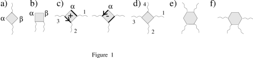
FIG. 1.: Hikami four-point and six-point vertices used. The wavy lines denote diffusons or cooperons. The current vertices are at the unoccupied corners of the polygons and are labeled by $\alpha$ and $\beta$.

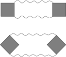
FIG. 2.: The UCF or $\langle g^{2}\rangle_{c}$ diagrams.

FIG. 3.: All basic topologies for the third cumulant diagrams. The wavy lines are diffusons or cooperons. The dots represent Hikami four point vertices. Detailed inspection of these diagrams will yield the diagrams of Fig. 4.

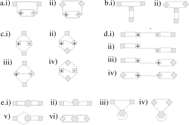
FIG. 4.: The calculated set of leading diagrams for the third cumulant of the conductance. The diagrams are derived from Fig. 3; one sees that structure is the similar. The diagrams e) are obtained by contraction of diffusons in the diagrams a), b), c) and d).

FIG. 5.: The third cumulant of the conductance multiplied by the average as a function of the transversal size in a 2D sample. Although the leading term vanishes in quasi 1D, it is non-trivial in 2D geometries.

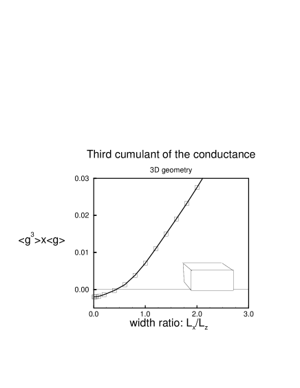
FIG. 6.: The third cumulant multiplied by the average conductance in 3D sample plotted against the transversal size $L_{x}$. The geometry is $L_{x}\times L_{z}\times L_{z}$ for the solid line. Note that, the sign changes in going from a quasi-2D to a 3D sample. The dashed line gives third cumulant in sample with geometry $L_{x}\times L_{x}\times L_{z}$ .

- [1] C. P. Umbach, S. Washburn, R. B. Laibowitz, and R. A. Webb, Phys. Rev. B 30, 4048 (1984).
- [2] P. A. Lee and A. D. Stone, Phys. Rev. Lett. 55, 1622 (1985).
- [3] B. L. Altshuler, JETP Lett. 41, 649 (1985).
- [4] B. L. Altshuler, V. E. Kravtsov, and I. V. Lerner, Sov. Phys. JETP 64, 1352 (1986).
- [5] B. Shapiro, Phys. Rev. Lett. 65, 1510 (1990).
- [6] B. L. Altshuler, V. E. Kravtsov, and I. V. Lerner, in Mesoscopic phenomena in solids, Vol. 30 of Modern problems in condensed matter sciences, edited by B. L. Altshuler, P. A. Lee, and R. A. Webb (North-Holland, Amsterdam, 1991), p. 449.
- [7] P. W. Anderson, D. J. Thouless, E. Abrahams, and D. S. Fisher, Phys. Rev. B 22, 3519 (1980).
- [8] A. A. Abrikosov, Solid State Comm. 37, 997 (1981).
- [9] V. I. Mel’nikov, Sov. Phys. Solid State 23, 444 (1981).
- [10] E. N. Economou and C. M. Soukoulis, Phys. Rev. Lett. 46, 618 (1981).
- [11] A. M. S. Macêdo, Phys. Rev. B 49, 1858 (1994).
- [12] M. L. Mehta, Random matrices and the statistical theory of energy levels (Academic Press, New York, YEAR).
- [13] A. V. Tartakovski, private communication.
- [14] A. V. Tartakovski, Phys. Rev. B 52, 2704 (1995).
- [15] M. C. W. van Rossum, J. F. de Boer, and Th. M. Nieuwenhuizen, Phys. Rev. E 52, 2053 (1995).
- [16] Th. M. Nieuwenhuizen and M. C. W. van Rossum, Phys. Rev. Lett. 74, 2674 (1995).
- [17] J. F. de Boer et al., Phys. Rev. Lett. 73, 2567 (1994).
- [18] A. Z. Genack and N. Garcia, Europhys. Lett. 21, 753 (1993).
- [19] C. L. Kane, R. A. Serota, and P. A. Lee, Phys. Rev. B 37, 6701 (1988).
- [20] M. C. W. van Rossum, Th. M. Nieuwenhuizen, and R. Vlaming, Phys. Rev. E 51, 6158 (1995).
- [21] P. A. Lee, A. D. Stone, and H. Fukuyama, Phys. Rev. B 35, 1039 (1987).
- [22] Th. M. Nieuwenhuizen, A. Lagendijk, and B. A. van Tiggelen, Phys. Lett. A 169, 191 (1992).
- [23] Th. M. Nieuwenhuizen and M. C. W. van Rossum, Phys. Lett. A 177, 102 (1993).
- [24] S. Hikami, Phys. Rev. B 24, 2671 (1981).
- [25] L. P. Gor’kov, A. I. Larkin, and D. E. Khmel’nitskii, JETP Lett. 30, 228 (1979).