RANDOMNESS AND APPARENT FRACTALITY

Abstract

We show that when the standard techniques for calculating fractal dimensions in empirical data (such as the box counting) are applied on uniformly random structures, apparent fractal behavior is observed in a range between physically relevant cutoffs. This range, spanning between one and two decades for densities of 0.1 and lower, is in good agreement with the typical range observed in experiments. The dimensions are not universal and depend on density. Our observations are applicable to spatial, temporal and spectral random structures, all with non-zero measure. Fat fractal analysis does not seem to add information over routine fractal analysis procedures. Most significantly, we find that this apparent fractal behavior is robust even to the presence of moderate correlations. We thus propose that apparent fractal behavior observed experimentally over a limited range in some systems, may often have its origin in underlying randomness.

1 Introduction

Fractal structures have been observed in a large variety of experimental systems in physics, chemistry and biology.[1, 2, 3, 4, 5, 6] Unlike exact (mathematical) fractals which are constructed to maintain scale invariance over many orders of magnitude, and most existing physical models displaying fractal behavior,[7] for empirical fractals the range over which they obey a scaling law is necessarily restricted by upper and lower cutoffs. In most experimental situations this range may be quite small, namely not more than one or two orders of magnitude (Fig.1). Nevertheless, even in these cases the fractal analysis condenses data into useful relations between different quantities and often provides valuable insight.

Figure 1: To obtain a general idea about the experimental status of fractal dimension measurements we collected all such measurements presented in Ref.[2] and measured the width of the linear range in the log-log plots (measured in decades) over which the FD was determined. This histogram shows the number of plots as a function of the number of decades of the linear range. One can see that most experimental measurements of fractal dimensions are based on data that extends between one and two decades. Note further that all the data with three and four decades, which come from a single paper, is the determination of the Hurst exponent for temporal and not structural data.          

Motivated by the yet inexplicable abundance of reported fractals, we consider here the apparent fractal properties of systems which are governed by uniformly random distributions. The reasons for this choice are several. First, randomness is abundant in nature. Second, although a uniformly random system cannot be fully scale invariant, it may, as we show below, display apparent fractality over a limited range, perhaps in better agreement with the actual ranges observed than a model which is inherently scale free. Third, a model of uniform randomness is a convenient limit, on top of which correlations can be introduced as perturbations.

2 The Basic Model

To illustrate our ideas we use a model that consists of a random distribution of spheres of diameter $d$, in the limit of low volume fraction occupied by the spheres. The positions of the centers of these spheres are determined by a uniform random distribution and the spheres are allowed to overlap. This model may approximately describe the spatial distribution of objects such as pores in porous media, craters on the moon, droplets in a cloud and adsorbates on a substrate as well as some energy spectra and random temporal signals.

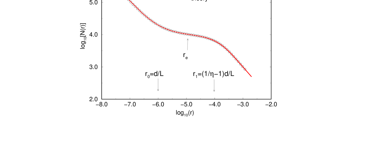
Figure 2: Comparison of simulation results (circles) to the theoretical prediction of Eq.(5) (solid line) for the number of intersected boxes as a function of their size, for one dimensional penetrable rods. The coverage is $\eta=0.01$ and the rod length is $d/L=10^{-6}$. The cutoffs are manifested as the two knees in the graph. The lower bound $r_{0}$ is seen to be located at $r=d/L$. The upper bound $r_{1}$ is at $r=(1/\eta-1)d/L$, also conforming with the prediction in the text. Also indicated is the estimated middle point $r_{e}$.          

To simplify the analysis we consider here (without loss of generality) the one dimensional case, where the spheres are $M$ rods of length $d$ which are placed on a line of length $L\gg d$. The positions of the rod centers are determined by a uniform random distribution. The rods are allowed to overlap and are positioned with no correlations. An information-theory argument can be used to show that this distribution is generic, or “minimal”, in the sense that it is characteristic of physical processes in which only the first moment (such as the density) is determined from outside.[8, 9] Below we calculate the fractal dimension (FD) of the resulting set using the box-counting (BC) procedure, which is a common techniques for determination of FD in empirical data.[10] In the BC technique one divides the embedding space into boxes of linear size $l$. It is convenient to work with the dimensionless quantity $r\equiv l/L$ for the box size. The number of boxes that have intersection with the measured object, $N(r)$, is then plotted vs. $r$ on a log-log scale. The range of $r$ is limited from below by the finest feature in the object and from above by the entire object size. Apparent fractal behavior is commonly declared in a range bound between physical cutoffs if the log-log plot of $N(r)$ vs. $r$ is linear over one or more decades[11] in that range. The dimension is given by:

$$D=-{\rm slope}\>\{\log(r),\log[N(r)]\}.$$ (1)

We will now show that our model generates approximate linearity over a range which would conventionally be accepted to indicate fractality. The lower cutoff is given by the rod length,

$$r_{0}=d/L,$$ (2)

since below this scale no new information is obtained by decreasing the box size. The upper cutoff is determined by the average distance between adjacent rod edges,

$$r_{1}=1/M-d/L,$$ (3)

because above this scale (on average) all boxes are occupied. This allows us to define an estimated scaling range as:[12]

$$\Delta_{e}=\log_{10}(r_{1})-\log_{10}(r_{0}).$$ (4)

Since the actual value of $N(r)$ depends on the particular set of random numbers drawn, one can only obtain the expectation value $\langle N(r)\rangle$. However, the law of large numbers ensures that for a large enough number of rods, the deviations from this value will be insignificant.

Following probabilistic arguments of the type used by Weissberg[13] and Torquato and Stell,[14] one obtains that out of the total of $1/r$ boxes the number of boxes that intersect the set is:[15]

$$\langle N(r)\rangle={1\over r}\left\{1-[1-(r+d/L)]^{M}\right\}.$$ (5)

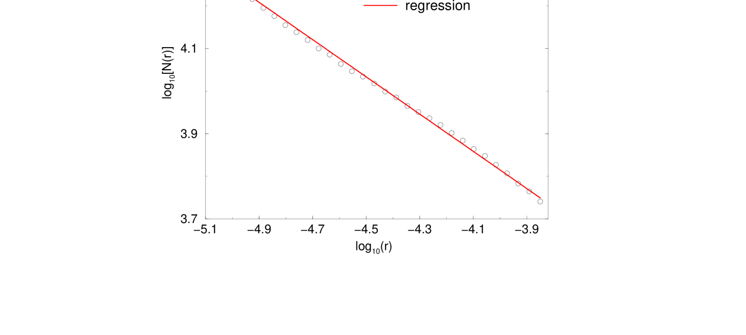
Figure 3: Simulation results (circles) for the number of intersected boxes $N(r)$ vs. $r$ in the experimentally relevant range (between cutoffs), along with a linear regression fit for coverage $\eta=0.1$ ($d/L=10^{-5},\,M=10^{4}$).          

Simulation results in terms of the coverage $\eta\equiv Md/L$ are shown in Fig.2, along with the theoretical prediction of Eq.(5). An excellent agreement is evident.[16]

Next, we examine the apparent FD [Eq.(1)], by mimicing the standard experimental procedure of using linear regression analysis between the cutoffs. The simulation results and the linear fit for $\eta=0.1$ are shown in Fig.3 for the range which is used to determine empirical FDs. More than a decade of linearity is observed for this high coverage. The slight inflexion of the simulation results may be smeared out by noise in a real experiment. We next evaluate the slopes and actual ranges of linearity $\Delta$ (generally $\neq\Delta_{e}$), under varying degrees of strictness of linearity, as measured by the coefficient of determination $R^{2}$. Typical results are shown in Fig.4, where, e.g. for $\eta=0.01$, more than two decades of linear behavior are exhibited for a required value of $R^{2}$ of below 0.975. This is well within the experimental norm as most experimental measurements of fractal objects do not extend for more than two orders of magnitude (Fig.1). Moreover, this agreement with experimental data is in contrast to that of most other physical models of fractality, which predict much larger ranges.[7] Increasing $\eta$ beyond 0.1 results in a decline of both $\Delta$ and $\Delta_{e}$ to below one decade and hence the apparent fractality is restricted to $\eta\leq 0.1$.

The results of the regression analysis for the apparent FD as a function of $\eta$ are shown in Fig.5 and are further compared to an analytical expression, obtained by calculating the logarithmic derivative of $N(r)$ at the estimated middle point $r_{e}=\sqrt{r_{0}r_{1}}$, in the $M\rightarrow\infty$, constant coverage limit:[8]

$$D=1-{\sqrt{\eta(1-\eta)}\over{\exp\left(\eta+\sqrt{\eta(1-\eta)}\right)-1}}.$$ (6)

As seen in Fig.5, the FD predicted by Eq.(6) is somewhat lower than the regression result and can serve as a lower bound. In the limit of small $\eta$, one can further simplify Eq.(6) and obtain

$$D\approx\left(\eta\over{1-\eta}\right)^{1/2},\ \ \ \ \ \ \eta\ll 1.$$ (7)

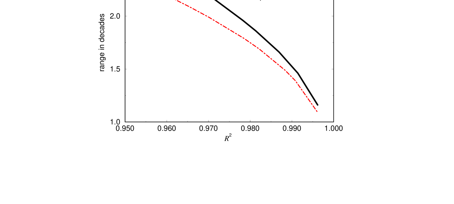
Figure 4: The range of linearity, $\Delta$, as a function of imposed coefficient of determination, $R^{2}$, in a linear regression analysis.          

3 Impenetrable Rods

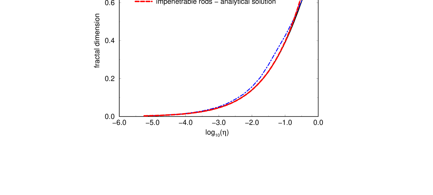
Figure 5: Apparent fractality (FD) as computed by linear regression with $R^{2}=0.995$ (upper curve). The predictions of the analytical equations, Eqs.(6) and (9) (for the penetrable and impenetrable rods) are accurate lower bounds and differ only marginally (two overlapping lower curves). This indicates the dominance of randomness over correlations.          

To examine the effect of correlations on the apparent FD we next consider a model in which rods are randomly located as before but with the restriction that the rods cannot overlap. The system is assumed to be at equilibrium. The excluded volume effect clearly creates correlations in the positions of the rods. This example is also fully solvable[8] and represents an important class of systems with correlations such as models of hard-sphere liquids and energy spectra with level repulsion. We will now show that the correlation introduced by the non-overlap restriction merely modifies the apparent fractal character of the system. For this case, the expected number of intersected boxes is:[8]

$$\langle N(r)\rangle={1\over r}\left(1-(1-\eta)\left(1-{r\over{1-\eta}}\right)^{M}\right).$$ (8)

Fig.6 shows the number of intersected boxes $\langle N(r)\rangle$ vs. $r$ both with [Eq.(5)] and without [Eq.(8)] overlap. The behavior in the two cases is qualitatively similar and virtually indistinguishable for low coverages. Fig.6 thus demonstrates that the apparent fractal behavior due to randomness is only slightly modified by moderate correlations. As in the overlapping rods case, we can now use Eq.(1) (with the slope calculated at $r=r_{e}$) to calculate a lower bound for the apparent FD. The result (for large $M$),

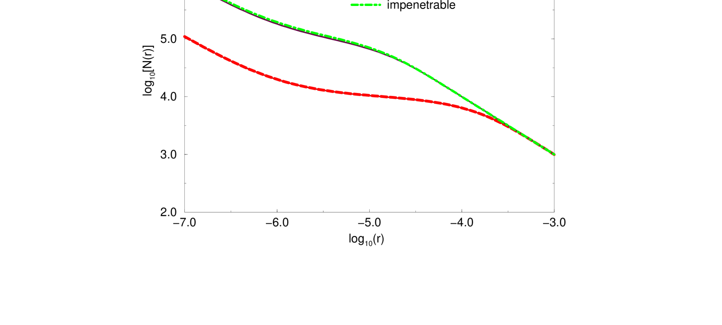
Figure 6: Comparison of box-counting predictions in penetrable and impenetrable rods cases. The results for penetrable [Eq.(5)] and impenetrable rods [Eq.(8)] virtually coincide for $\eta\leq 10^{-2}$ (lower two curves). For $\eta=0.1$ a barely noticeable difference develops (upper two curves). In both cases $d/L=10^{-6}$.          

$$D=1-{{\eta\sqrt{{1/\eta}-1}}\over{\exp\left(\sqrt{\eta/(1-\eta)}\right)-(1-\eta)}}$$ (9)

is shown in Fig.5. The important observation is that for a broad range of low coverages the apparent FD’s of penetrable and impenetrable rods nearly overlap. This is the relevant range for fractal measurements and therefore we find that correlations of the type considered here have little effect on the apparent fractal nature of the system.

4 Fat-Fractal Analysis

In this section we treat the penetrable spheres model for the case of two-dimensional (2D) disks, from the point of view of fat-fractal analysis. A fat fractal is defined as “A set with a fractal boundary and finite Lebesgue measure”.[17] The fat-fractal approach is natural for our model, since the set of disks clearly has non-zero measure. Fat-fractal analysis can be performed on experimental data (but rarely is) in those cases where the resolution of the measurement device is finer than the lower cut-off, which is required for a knowledge of the measure of the studied set. An example is helium scattering.[18] In the present case we show that the measure of the set of disks can be found analytically. In order to measure the fat-fractal scaling exponent $\gamma$, one performs, as in the standard fractal analysis, a box-counting procedure:

$$\gamma=\lim_{r\rightarrow r^{*}}{{\log[A(r)]}\over\log(r)}\>;\>\>\>\>A(r)\equiv r^{2}N(r)-\mu_{0},$$ (10)

where $\mu_{0}$ is the normalized Lebesgue measure of the set. The fractal dimension itself is given by

$$D_{ff}=2-\gamma.$$ (11)

In the nonlinear dynamical systems literature, where fat fractals were first introduced,[19] $r^{*}=0$. In the context of real-space sets, there exists a lower cutoff $r_{0}>0$, and hence also $r^{*}>0$. One should bear this in mind whenever fractal theory is applied to real-space systems with an inherent non-vanishing smallest scale.

Consider then again a system of $M$ uniformly randomly positioned disks of equal radius $R=d/2$, located at low 2D coverage $\eta_{2}$ given by:

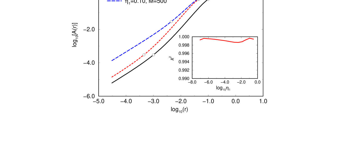
Figure 7: Fat fractal analysis of random disks. Analytical results of Eq.(10) for $A(r)$ are shown at three combinations of coverages $\eta_{1}$ and disk numbers $M$. Circles indicate the positions of the cutoffs according to Eqs.(2),(3). Inset: Linear regression coefficient ${\cal R}^{2}$ for regression in-between the cutoffs.          

$$\eta_{2}=M\pi R^{2}/L^{2}=(\pi/4)\eta_{1}^{2},$$ (12)

on a surface of area $L^{2}$. The effective “1D coverage”

$$\eta_{1}=\sqrt{M}2R/L,$$ (13)

is defined for convenience of comparison with results in 1D and 3D. In order to find $\mu_{0}$, imagine that the surface is initially empty, and randomly choose a point on it. Next locate a disk of radius $R$ at a random position on the surface. The probability that it does not include the chosen point is proportional to the free area, namely $q_{1}=(L^{2}-\pi R^{2})/L^{2}$. The next disk is also positioned completely randomly, so that the probability for the point to be outside of both disks is just $q_{1}^{2}$. Clearly, after random placement of $M$ disks, the point will lie in the uncovered region with probability $q_{1}^{M}$, and therefore will be in the disk-covered region with probability $p_{M}=1-(1-\pi R^{2}/L^{2})^{M}$. On the other hand, this probability is just the expectation value of the normalized disk union area, $\mu_{0}/L^{2}$. Thus for large enough $M$:[13, 14]

$$\mu_{0}=\left[1-(1-\pi R^{2}/L^{2})^{M}\right]L^{2}.$$ (14)

A modified argument can be used to evaluate the BC function for our basic model.[8] The result for the expected number of occupied boxes is:

$$N(r)={L^{2}\over r^{2}}\left[1-\left(1-r^{2}-4r\,R/L-\pi(R/L)^{2}\right)^{M}\right].$$ (15)

Simulations[8] (not shown here) confirm the 1D version of this result to excellent accuracy for $M$ as small as 100. Taken together, Eqs.(14),(15) determine the fat-fractal exponent $\gamma$, using Eq.(10). Analytical results are shown in Fig.7 for three $\eta_{1}/M$ pairs. The effect of changing $M$ at constant coverage (solid and short-dashed lines) is a rigid translation of the curve in the plane. This implies that the coverage is the important parameter in determining the slope i.e., the FD. Circles indicate the positions of the cutoffs according to Eqs.(2),(3). Beyond the lower cutoff the slope tends to 1, beyond the upper cutoff – to 0. In-between the cutoffs, a nearly straight line is observed, in agreement with apparent fractal behavior. In order to find $\gamma$ it remains to determine the point $r^{*}$. For disks, in analogy to the discussion for rods, the cutoffs are given by:

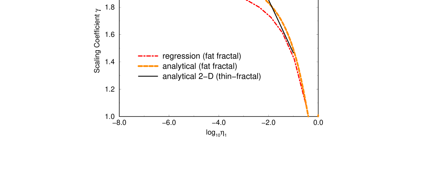
Figure 8: Analytical and regression slope between the cutoffs (dashed and long dashed) of fat fractal analysis, and $2\!-\!D$ of “thin” fractal analysis.          

$$r_{0} = 2R/L$$

$$r_{1} = 1/\sqrt{M}-2R/L.$$ (16)

As in Sec.2 we choose $r^{*}$ as the estimated middle point of the scaling range,

$$r^{*}=r_{e}=\sqrt{r_{0}\,r_{1}},$$ (17)

and find $\gamma$ by evaluating the logarithmic derivative of $A(r)$ there. The result is:

$$\gamma={{d\log[A(r)]}\over{d\log(r)}}\left|{}_{r_{e}}\right.={{2\eta_{1}(1-\eta_{1}+\sqrt{\eta_{1}-\eta_{1}^{2}})}\over{\exp[\eta_{1}(1-\eta_{1}+2\sqrt{\eta_{1}-\eta_{1}^{2}})]-1}}.$$ (18)

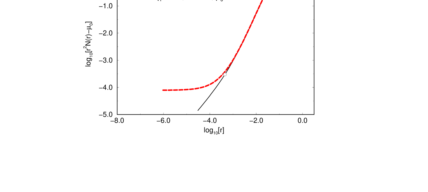
Figure 9: Log-log plot of $A(r)=r^{n}N(r)-\mu_{0}$ (solid line) and just $r^{n}N(r)$ (dashed line). Inside the physical range, the measure $\mu_{0}$ has little effect. Circles indicate the cutoffs.          

This result is compared in Fig.8 to the result of the regular (“thin”) fractal analysis, for which we found:[8]

$$2-D={{{1\over 2}[\eta_{1}\sqrt{2\eta_{1}-\eta_{1}^{2}}+2\eta_{1}-\eta_{1}^{2}]}\over{\exp\{\eta_{2}+{1\over 2}[\eta_{1}\sqrt{2\eta_{1}-\eta_{1}^{2}}+{1\over 2}(2\eta_{1}-\eta_{1}^{2})]\}-1}}.$$ (19)

The two curves differ only slightly. The analytical fat-fractal result is also compared in Fig.8 to the procedure followed in typical experimental analysis of fractal scaling data: a linear regression between the physical cutoffs ($r_{0}$ and $r_{1}$ in our case). The trend is similar, and the agreement is quite good for the higher coverages. In any case the analytical Eq.(18) serves as an accurate upper bound to the expected regression result for $\gamma$. The corresponding regression coefficient ${\cal R}^{2}$ (inset of Fig.7) does not fall below 0.9985 which indicates a very high quality regression, certainly by experimental standards. Note that ${\cal R}^{2}$ remains very high even for $\eta_{1}<10^{-2}$ (i.e., a scaling range $\Delta_{e}>2$). This is a wider range than found for the 1D version of “thin” fractal analysis. There the apparent fractality was observed in a range of 1-2 decades if $\eta<10^{-1}$ and ${\cal R}^{2}>0.97$ are required (Fig.4). This range improvement is not a direct outcome of the inherent fractality we found between the cutoffs, but is due to the differences in the response of the linear regression procedure to Eq.(10), in comparison to Eq.(1): It is the multiplication of the BC function by $r^{2}$ in the former which is responsible for the improved range effect, through the increase in the slope of the log-log plot. One should be cautious therefore to eliminate slope-biases in analyses of scaling properties on a log-log plots. Furthermore, as clearly seen in Fig.9, the essence of the fat fractal analysis, namely the subtraction of the measure $\mu_{0}$ of the set, has essentially no effect on the slope and on the location of the cutoffs and thus does not provide us in this case with added information. Being left then with the choice between $N(r)$ and $r^{2}N(r)$, there does not seem to be a clear reason to opt for the latter. We conclude that for low density systems, such as in this report, fat fractal analysis is not necessary.

5 Conclusions

In summary, we have shown that random structures, which are generic in experimental situations where only the first moment of a distribution is determined, give rise to apparent fractal behavior within physically relevant cutoffs, with a non-universal FD. Although this is not a mathematically rigorous fractality, in the sense that the scaling is not strictly a power law, it is a physical fractality: It satisfies the conditions of high-quality linear regression in the physically relevant range of observation. Since experiments rarely observe a perfect power law, we believe that the possibility of approximate scaling should be considered in theoretical models, if a more complete understanding of the experimental fractal data is to be achieved. It is likely that some of this data does in fact not reflect the existence of an exact power law, but rather an approximate power law between cutoffs with a weak inflexion point in the log-log plot. The present model and its approximate scaling properties hint that this may be the case, e.g., for porous media. Moderate correlations have little effect on the apparent fractal properties and even in their presence it is still the underlying randomness that is the main contributor to the apparent power-law scaling relation. Elsewhere we showed that these results remain practically unchanged for higher dimensions and for a variety of size distribution profiles of the elementary building blocks.[8] We thus propose to consider randomness as a possible common source for apparent fractality.

References

References

- [1] B. B. Mandelbrot. The Fractal Geometry of Nature. Freeman, San Francisco, 1982.
- [2] J. Feder and A. Aharony, editor. Fractals in Physics, Essays in Honour of B.B. Mandelbrot. North Holland, Amsterdam, 1990.
- [3] D. Avnir, editor. The Fractal Approach to Heterogeneous Chemistry: Surfaces, Colloids, Polymers. John Wiley & Sons Ltd., Chichester, 1992.
- [4] A. Bunde, S. Havlin, editor. Fractals in Science. Springer, Berlin, 1994.
- [5] H. E. Stanley, N. Ostrowsky, editor. On Growth and Form. Number 100 in NATO ASI Ser. E. Martinus Nijhoff, Dordrecht, 1986.
- [6] M. Schroeder. Fractals, Chaos, Power Laws. W.H. Freeman, N.Y., 1991.
- [7] Such models include for example: diffusion limited aggregation (T. A. Witten and L. M. Sander, Phys. Rev. Lett. 47, 1400 (1981)); percolation models (see e.g., D. Stauffer, Introduction to Percolation Theory, Taylor and Francis, London, 1985); and sand pile models which exhibit self organized critical behavior (P. Bak, C. Tang and K. Wiesenfeld, Phys. Rev. Lett. 59, 381 (1987)).
- [8] D.A. Hamburger, O. Biham and D. Avnir. Phys. Rev. E. 53, 3342 (1996).
- [9] Similar arguments were used recently [C. Tsallis, S.V.F. Levy, A.M.C. Souza and R. Maynard, Phys. Rev. Lett. 75, 3589 (1995)] to argue for the ubiquity of Lévy distributions in Nature. There it is the second moment which is imposed as a constraint in an information theoretic argument.
- [10] We have also applied the “Minkowski Sausage” technique. In one dimension the two methods naturally provide identical results while we found that in two and three dimensions they slightly differ.[8] Both methods measure . Elsewhere we will treat the case of , .
- [11] P. Pfeifer and M. Obert, in Ref.[3], p.16.
- [12] Many authors report their results on a or scale, which may give a misleading impression of a larger scaling range than is actually available. We urge that all results are reported on a scale.
- [13] H.L. Weissberg. J. Appl. Phys.34, 2636 (1963).
- [14] S. Torquato, G. Stell. J. Chem. Phys. 79, 1505 (1983).
- [15] The idea is to pick one box and then randomly deposit rods of size on the unit interval. The probability that the chosen box remains empty is and thus the probability that it will intersect at least one rod is .
- [16] This excellent agreement appears for all scales in including the ranges of slope=1. This was also confirmed for other choices of and values and even for very large where apparent fractal behavior is not seen.
- [17] R. Eykholt and D.K. Umberger. Physica D 30, 43 (1988).
- [18] D.A. Hamburger, A.T. Yinnon and R.B. Gerber. Chem. Phys. Lett. 253, 223 (1996).
- [19] D.K. Umberger and J.D. Farmer. Phys. Rev. Lett. 55, 661 (1985).